| Issue |
A&A
Volume 618, October 2018
|
|
|---|---|---|
| Article Number | A67 | |
| Number of page(s) | 7 | |
| Section | Galactic structure, stellar clusters and populations | |
| DOI | https://doi.org/10.1051/0004-6361/201833929 | |
| Published online | 12 October 2018 | |
The possible common origin of M 16 and M 17⋆
1 European Southern Observatory, Karl-Schwarzschild-Str. 2, 85748 Garching bei München, Germany
e-mail: fcomeron@eso.org
2 Institut de Ciències del Cosmos (ICCUB-IEEC), Barcelona 08028, Spain
Received:
23
July
2018
Accepted:
6
August
2018
Context. It has been suggested that the well-studied giant HII regions M 16 and M 17 may have had a common origin, being an example of large-scale triggered star formation. While some features of the distribution of the interstellar medium in the region support this interpretation, no definitive detection of an earlier population of massive stars responsible for the triggering has been made thus far.
Aims. We have carried out observations looking for red supergiants in the area covered by a giant shell seen in HI and CO centered on galactic coordinates l ∼ 14°5, b ∼ +1° whose emission peaks near the same radial velocity as the bulk of the emission from both giant HII regions, which are located along the shell. Red supergiants have ages in the range expected for the parent association whose most massive members could have triggered the formation of the shell and of the giant HII regions along its rim.
Methods. We have obtained spectroscopy in the visible of a sample of red stars selected on the basis of their infrared colors, whose magnitudes are consistent with them being red supergiants if they are located at the distance of M 16 and M 17. Spectroscopy is needed to distinguish red supergiants from AGB stars and RGB stars, which are expected to be abundant along the line of sight.
Results. Out of a sample of 37 bright red stars, we identify four red supergiants that confirm the existence of massive stars in the age range between ∼10 and ∼30 Myr in the area. At least three of them have Gaia DR2 parallaxes consistent with them being at the same distance as M 16 and M 17.
Conclusions. The evidence of past massive star formation within the area of the gaseous shell lends support to the idea that it was formed by the combined action of stellar winds and ionizing radiation of the precursors of the current red supergiants. These could be the remnants of a richer population, whose most massive members have already exploded as core-collapse supernovae. The expansion of the shell against the surrounding medium, perhaps combined with the overrun of preexisting clouds, is thus a plausible trigger of the formation of a second generation of stars currently responsible for the ionization of M 16 and M 17.
Key words: stars: early-type / ISM: bubbles / HII regions / ISM: individual objects: M 16 / ISM: individual objects: M 17
© ESO 2018
1. Introduction
The close proximity in the sky of M 16 and M 17, two of the nearest giant HII regions of our galactic neighborhood lying at a similar distance from the Sun, naturally leads to the question of whether they are physically related, and whether they may share a common origin (Moriguchi et al. 2002; Oliveira 2008; Nishimura et al. 2017). Both giant HII regions are projected on the contour of a giant bubble-shaped structure, outlined in the distribution of HI and CO emission as first noted by Moriguchi et al. (2002). Evidence for triggered star formation in M 16 has been examined in detail by Guarcello et al. (2010), who concluded it had been induced externally, and not by the activity of its associated cluster NGC 6611. This suggests that the formation of M 16 and M 17 could have been triggered by the expansion of the bubble, powered by a previous generation of massive stars near its center, thus representing an example of triggered star formation on the scale of several tens of parsecs (Elmegreen 1998). Given the ages of the giant HII regions, the timescale of expansion of a wind-blown bubble, and the short lifetimes of massive stars, it is to be expected that the most massive members of that previous generation may have exploded as supernovae several Myr ago. The spatial dispersion of the members of the association that must have taken place progressively during its existence, combined with the distance of 2 kpc to the M 16–M 17 complex and the large number of unrelated foreground and background stars in that general direction, would make it extremely difficult to identify even its currently hottest members still remaining on the main sequence. Moriguchi et al. (2002) noted the presence of O and early B stars in the area and proposed that they were part of a massive star population responsible for having caused the bubble, but a review of their properties shows them to be generally too bright to be at the distance of the bubble and the giant HII regions, and instead are more likely members of a foreground population.
Red supergiants stars offer a venue to circumvent this problem. They are the descendants of stars with initial masses between 7 and 40 M⊙ (Hirschi et al. 2010), which reach this phase after leaving the main sequence at ages ranging from 5 Myr to 50 Myr, the precise value depending on both the initial mass and the initial rotation velocity (Ekström et al. 2012). The duration of the red supergiant phase ranges from several hundred thousand years to about 2 Myr. Although relatively short-lived, red supergiants are found in significant numbers in rich stellar aggregates with ages extending up to a few tens of Myr, and their luminosity makes them stand out at near-infrared wavelengths, therefore making them suitable and easily accessible probes of past massive star formation in regions where O-type stars have already completed their life cycles (Davies et al. 2007; Clark et al. 2009; Messineo et al. 2014; Negueruela 2016; Alegría et al. 2018).
Here we present the results of a search for the vestiges of the massive stellar association that could have triggered the formation of the shell containing M 16 and M 17 through the identification of red supergiants in the area. We present our target selection criteria and our findings, through which we produce a crude estimate of the overall massive star content of the association and the mechanical energy deposited in the bubble, which suggest that the scenario of triggered formation of M 16 and M 17 is indeed plausible.
2. Target selection
M 16 and M 17 are giant HII regions located at similar distances from the Sun. The distance to M 16 has been estimated to be 1.8 kpc (Oliveira 2008; and references therein), while that of M 17 has been determined to be  (Xu et al. 2011) through the VLBI trigonometric parallax of masers associated with its massive star formation sites. The ages have been estimated at less than 3 Myr for M 16 (e.g., Guarcello et al. 2012) and 1 Myr or less for M 17 (e.g., Hanson et al. 1997), although evidence of an older population in the former region has been reported by De Marchi et al. (2013). The average radial velocities of the ionized gas in both regions are similar, νLSR = +26.3 km s−1 for M 16 and νLSR = +16.8 km s−1 for M 17 (Lockman 1989). Extensive reviews on each of these regions can be found in Oliveira (2008) and Chini & Hoffmeister (2008).
The large shell-like disturbance noted by Moriguchi et al. (2002) is clearly seen in the data extracted from the galactic HI atlas of Hartmann & Burton (1997) and the galactic disk CO atlas of Dame et al. (2001) at radial velocities +15 ≲ νLSR(km s−1) ≲ +20 between galactic longitudes 12° ≲ l ≲ 18°, centered near l ∼ 14°5, b ∼ +1°. Both M 16 and M 17 lie along the rim of the shell, which is incomplete at high galactic longitudes, perhaps indicating that it has formed a chimney-like structure venting gas to the galactic halo. There are no known star clusters possibly associated with the bubble. Of the four star clusters projected on the area listed by Dias et al. (2002) and the successive updates of their calalog, three have estimated ages in excess of 250 Myr. The fourth cluster, NGC 6561, is listed as having an age of 8 Myr, but at 3.4 kpc it is too distant to be physically associated with the region under study.
We used the 2MASS All-Sky data release (Skrutskie et al. 2006) to produce a sample of targets for spectroscopic follow-up. A total of 37 stars with KS < 4.8, J − KS > 1.1 were selected in the rectangle defined by the galactic coordinates 13° ≲ l ≲ 16°,
0° ≲ b ≲ 2°. The KS magnitude limit corresponds to a red supergiant with absolute magnitude MK = −7.7 at a distance modulus of 11.5 mag, obscured by a foreground extinction AK = 1 mag. The J − KS color limit ensures that red supergiants with virtually no foreground extinction are also included in our sample. The sample is expected to be considerably contaminated by foreground red giant branch (RGB) stars, asymptotic giant branch (AGB) stars, and perhaps other types of cool stars, thus requiring spectral classification to confirm the presence of red supergiants.
3. Observations and spectral classification
We obtained spectra of the 37 stars in our sample using CAFOS, the facility imager and low-resolution spectrograph at the 2.2 m telescope of the Calar Alto Observatory, on the nights of 22–23 and 23–24 June 2018. A single spectroscopic configuration was used consisting of a grism providing a coverage over the 5900−9000 Å range and a slit width of 1″5, yielding a resolution R = 1300. Exposure times were adjusted according to the red magnitude of the target, ranging from 120 s to 1800 s. The spectra were reduced and extracted using standard IRAF tasks, and calibrated in wavelength using the internal Hg, He and Rb arc lamps in the calibration unit of the instrument.
Spectral classification was carried out by using a grid of MK standards obtained from the catalog of Garcia (1989) covering spectral types K2 to M4 (the latter corresponding to the temperatures of the coolest red supergiants) and luminosity classes Ia to III, which were observed with an identical instrument setup and reduced in the same way as our target observations. The grid of comparison standards is presented in Table 1. Many of our targets turned out to be very late-type giants with temperatures and spectral types below the range covered by red supergiants, which we classified for the sake of completeness using the atlas presented in Fig. 7 of Fluks et al. (1994).
Grid of MK standards used for classification.
The differences between red supergiants and luminosity class III giants in the spectral range K0–M4 in the wavelength region covered by our spectra are rather subtle. The problem has been studied in detail by Dorda et al. (2016, 2018) using principal component analysis on large samples of luminous red stars. For the spectral range and resolution of our spectra, a convenient and highly reliable criterion is based on selected surface gravity-sensitive lines in the calcium triplet region, already noted by Keenan & Hynek (1945). We used for this purpose the KI lines at 7665 Å and 7699 Å and the FeI lines at 8468 Å (blended with Ti), 8514 Å and 8469 Å, all of which have a positive luminosity class effect. We measured their equivalent widths in the spectra of both our targets and the MK standards, and used the sum of equivalent widths of all five features to identify the red supergiants in our sample. Figure 1 shows the separation of the MK standards between giants and supergiants reflected in the sum of equivalent widths and the positions of our targets in the same plot, where we can see that four of the stars, J18143590–1621473, J18145920–1707138, J18145951–1614573, and J18182574–1518131, appear well in the region occupied by red supergiants. The measured equivalent widths are given in Table 2, together with the spectral classifications of the whole sample, and their locations are shown in Fig. 2.
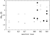 |
Fig. 1. Sum of the equivalent widths of the five luminosity-sensitive spectral features noted in Table 2, both for the MK standards listed in Table 1 and for our targets stars with spectral types M4 or earlier. Squares represent luminosity class Ia standards; triangles, class Iab; open circles, class Ib; crosses, class II; and asterisks, class III. The filled circles correspond to our targets. We consider the four stars with a sum of equivalent widths above 2.5 as bona fide supergiants, as no class III standard populates that region. |
Spectral classification and equivalent widths of luminosity-sensitive features.
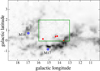 |
Fig. 2. Map of CO emission in the velocity range +15 ≲ νLSR(km s−1) ≲ +20, showing the open shell that dominates the distribution between 13° < l < 18° and the positions of the giant HII regions M 16 and M 17 superimposed on its rim. The rectangle marks the area where we selected red supergiant candidates, and the four circles show the locations of the four confirmed red supergiants that we have found. |
The trigonometric parallax measurements of J18145951–1614573 and J18182574–1518131 are listed respectively as 0.4751 ± 0.1689 mas and 0.4935 ± 0.1044 mas in the Gaia DR2 catalog (Gaia Collaboration 2018), in excellent agreement with the estimated distances to M 16 and M 17 quoted in Sect. 2. A third star, J18145920–1707138, also has a parallax consistent with that distance, 0.7037 ± 0.2863 mas, well within its error bar. The parallax of the fourth star, J18143590–1621473, is listed as 0.1472 ± 0.0951 mas, suggesting a much greater distance of over 4 kpc, or even 6.8 kpc at the central value of 0.1472 mas. The temperature and luminosity implied by such a distance is still within the range allowed by evolutionary models that we discuss in Sect. 4.1, but we note that this star is within only 8′9 of J18145951–1614573, one of the two stars whose parallax best matches the distance to M 16 and M 17, and has an even lower amount of foreground extinction. We thus consider it more likely that it is part of the complex under study, rather than being a background supergiant.
Two other stars, J18142432–1707379 and J18153653–1614197, have a sum of equivalent widths marginally above the narrow band defined by giants (see Table 2). This region is also populated by a few class I and II giants. To discern their true nature, we note that the parallax measured by Gaia for J18153653–1614197 is 1.0153 ± 0.0653, thus strongly suggesting that it is a foreground red giant. Concerning J18142432–1707379, the Gaia DR2 catalog lists a negative parallax (−0.3415 ± 0.3103), suggesting problems with the measurements. We do not consider either star among our sample of red supergiants.
4. Results
4.1. Physical parameters
We used the intrinsic colors of galactic red supergiants of Elias et al. (1985) to estimate the extinction and absolute magnitude MK of all four red supergiants, assuming a common distance modulus for all of them. Temperatures and bolometric corrections were derived using the calibrations of Levesque et al. (2005) and Levesque et al. (2007) for galactic red supergiants. The extinction estimate was made from the (V − KS) color using the 2MASS KS magnitude and the V magnitude listed in the NOMAD catalog (Zacharias et al. 2004). The positions of the stars in the temperature–luminosity diagram were then compared with the Geneva evolutionary tracks for massive stars with and without rotation (Ekström et al. 2012), as shown in Fig. 3. Initial masses and ages were then derived by assuming that all the stars are on the steady evolutionary part of its evolutionary track, corresponding to the phase of helium burning at the core, before the upturn immediately preceding the supernova explosion or, for rotating stars, before the blue loop excursion to higher temperatures that follows the end of He burning. Although taken at face value the temperatures adopted for the stars places them right on the upturn, the very short duration of that stage leads us to believe that this is almost surely due to a mismatch between the temperatures predicted by the evolutionary tracks and the temperature calibration, in the sense of the latter being colder. The difficulties and uncertainties in the determination of galactic red supergiant temperatures have been discussed by Levesque et al. (2005).
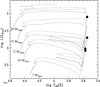 |
Fig. 3. Position of the four red supergiants on the temperature–luminosity diagram. The Geneva evolutionary tracks (Ekström et al. 2012) are plotted for stars with different initial masses, both non-rotating (solid lines) and rotating with a velocity 40% of the critical velocity. |
Table 3 lists the derived physical parameters of each star, for the two cases of a non-rotating precursor and of a precursor rotating at 0.4 times the critical velocity. Rotation produces a moderate increase of the luminosity for a star of a given mass, a longer duration of the main sequence phase, and a slightly longer duration of the He burning phase. The presence in the region of supergiants with widely different luminosities, and therefore widely different ages, implies an extended star forming period.
Parameters of red supergiants.
4.2. Estimating the number of massive stars and supernovae
Given the short duration of the red supergiant phase, the fact that we can observe four stars undergoing this phase simultaneously hints at a large number of precursors during the star formation history of the region. We can use the number of currently observed M supergiants, together with simple assumptions on the star formation rate and a standard initial mass function, to obtain a crude estimate of the number of massive stars that have existed in the region and the number of core-collapse supernovae that have happened, leading to an estimate of the mechanical energy dumped into the bubble.
The expected number of red supergiants NRSG observed at present (t = 0) can be expressed as
where Ψ(t) is the star formation rate, ξ(M) is the initial mass function, A is a normalization factor, and VRSG(M, t) is a visibility function: VRSG(M, t) = 1 if a star of mass M formed at time t is at the red supergiant phase at present, and zero otherwise1.
We make the rough assumption that Ψ(t) was constant during the whole period in which the stars currently observed as red supergiants were born. We further assume, rather conservatively, that the star formation history of the region extends from the time of formation of the least massive red supergiant observed at present until the time when the most massive red supergiant now visible formed. Assuming that the star formation history is limited in this way makes the limits of the integration over time and mass largely irrelevant, as the expression within the integral has a value of zero for masses below that of the least massive red supergiant, and also for masses above that of the most massive one. Adopting a power law with the Salpeter exponent −2.35 for the high-mass end of the initial mass function, ξ(M) = M−2.35, the current observation of NRSG = 4 sets the value of the normalization factor A.
The number of massive stars down to a mass Mlim that have formed in the region, which we denote as NOB for convenience (although Mlim does not necessarily have to correspond to the mass of a B star), can be expressed in terms of the quantities introduced in the previous equation:
Using Eq. (1),
Calculated in this way NOB includes all the stars down to mass Mlim that have formed in the region, regardless of whether the star still exists or has already exploded as a supernova. If Mlim is chosen such that the lifetime of a star of that mass is shorter than the time in the past when star formation in the region ceased, no stars with a mass higher than Mlim should be observable at present in the region. To estimate the total number of supernovae NSN a similar expression can be written:
where MSN is the minimal initial mass for a star to end its life as a core collapse supernova, for which we adopt M = 8 M⊙. Here VSN(M, t) has a value of zero if the absolute value of t is less than the lifetime of a star of mass M, and unity otherwise.
Using NRSG = 4 and the ages listed in Table 3, we estimate the number of O-type stars that existed in the history of the association (down to M = 17.5 M⊙; Pecaut & Mamajek 2013) to be between 29 (adopting ages from models with no rotation) and 37 (rotation with ν = 0.4νcrit). The number of core collapse supernovae is estimated to be between NSN ∼ 82 (no rotation) and 111 (with rotation). Given the old age of the lightest red supergiants currently observed in the region, we expect that a large number of stars with early B-type precursors (M < 17.5 M⊙) have already exploded as supernovae.
4.3. Bubble energetics
A similar computation allows us to estimate the energy dumped inside the bubble blown around the ancient association by OB stars and supernovae. The kinetic energy deposited inside the bubble by stellar winds is
where  is the mechanical luminosity of the wind of a star of mass M having a mass loss rate Ṁ and a terminal wind velocity ν∞. τ(M) is the time over which the star has been producing the wind: τ(M) = min(−t, τOB(M)), where τOB(M) is the main sequence lifetime of a OB star of mass M. We neglect the short-lived Wolf–Rayet and blue supergiant phases as their overall contribution to the energetics of the bubble is comparatively small, as well as the red supergiant phase in which the slow wind makes the contribution to the mechanical luminosity integrated over time irrelevant. We have used the compilation of data of OB stars with normal winds by Martins et al. (2005) to derive empirical log Ṁ− log L and
  relations, where L is the luminosity of the star and R is its radius, which we derive from the log L and log Teff values for stars of different masses compiled by Pecaut & Mamajek (2013).
The integration of Eq. (5) leads us to estimate Ewind ∼ 1052 erg. The decrease in both Ṁ and ν∞ with decreasing stellar mass implies that Ewind is dominated by high-mass stars, in spite of the declining initial mass function and main sequence lifetimes with increasing mass. Under our assumption that massive star formation in the region ended at the time when the most massive red supergiant currently observed was born, the contribution of stellar winds to the bubble energetics ceased to be important long ago, as the most massive stars with the most powerful winds ended their main sequence life. On the other hand, stars with lower masses formed over the history of the region have continued to explode as core-collapse supernovae until the present, and currently dominate the rate of injection of energy into the bubble. Adopting a kinetic energy of 1051 erg per supernova, the numbers given in Sect. 4.2 suggest an energy input of ∼1053 erg due to supernovae.
Within the rough approximations and extrapolations made, the energy dumped by stellar winds and (mainly) supernovae in the interior of the bubble appears to be sufficient for it to have rearranged the molecular gas in the region over the large region delineated by the contour of the CO shell. If the bubble were powered by the energy deposited at a roughly continuous rate over a period of 30 Myr and expanding in a uniform medium of density n0, its radius at present would be
(e.g., Bisnovatyi-Kogan & Silich 1995, and references therein), where Lm is the kinetic energy injected in the bubble per unit time, which we approach as Lm ∼ 1053erg/30 Myr ∼ 1038erg s−1 and t is the current age of the bubble, which we take as 30 Myr. If the original association formed in a giant molecular cloud with the typical average density n0 ∼ 100 cm−3, the expected radius of the bubble would be on the order of R ∼ 200 pc. This is significantly larger than the actually measured ∼ 70 pc, but the discrepancy should not be taken as ruling out the interpretation of the shell as the edge of the bubble blown by the massive members of the old association: the stellar and supernova content of the association and the duration and history of the star forming activity are two of the main unknowns where we have made educated guesses rather than accurate reconstructions. The history of star formation, and therefore of the injection of mechanical energy, can strongly influence the pattern of expansion of a bubble (Silich 1996). Furthermore, the radius derived from Eq. (6) exceeds the vertical scale height of the HI layer of the galactic disk (Dickey & Lockman 1990), and the effect of evolution in a density-stratified medium is obvious in the shape of the shell, which strongly suggests that the bubble has blown up and has vented much of the energy into the galactic halo. Concerning the expansion velocity of the shell, ν = dR/dt, the adopted quantities yield  , close to the sound speed in the warm interstellar medium, implying that the expansion of the shell still causes a strong compression of the swept-up gas.
5. Discussion and conclusions
We have developed the interpretation of the presence of four red supergiants in the interior of the shell in whose rim M 16 and M 17 are located as an indication for the past existence of a rich OB association in the region. The association, which formed massive stars over an extended period lasting from ∼30 Myr to ∼10 Myr ago, may have hosted several tens of O stars and the precursors of around one hundred supernovae up to the present time. Such an extended period of star formation may not be an anomalous feature of large, rich OB associations, based on similar recent findings on the younger, more nearby Cygnus OB2 association (Hanson 2003; Comerón & Pasquali 2012; Comerón et al. 2016; Berlanas et al. 2018).
Our estimates about the richness of the association and its supernova history involve some grossly oversimplifying assumptions, and should not be taken as a quantitative proof of the hypothesis. However, we have shown that the injection of mechanical energy into the bubble by the postulated association could have produced a substantial rearrangement of the gas on scales of over a hundred parsec, accounting for the current size of the shell, and an expansion at supersonic speeds up to the present, thus being able to compress the swept-up gas or previously existing gas concentrations encountered along the path of expansion, ultimately triggering additional star formation. The origin and location of M 16 and M 17, two giant HII regions much younger than the estimated age of the old association, as a consequence of triggered star formation along the rim of the shell thus becomes a plausible scenario. A more realistic modeling should take into account at least a time-variable energy input consistent with the assumed star formation rate of the association and the expansion of the shell in a vertically stratified medium.
Proposed examples of triggered star formation abound in the literature over a variety of scales. In particular, the high–quality infrared observations from the Spitzer and Herschel space observatories over the last decade and a half have provided abundant support for the actual existence of triggered star formation along the edges of bubble-like HII regions (Deharveng & Zavagno 2011; Samal et al. 2014; Liu et al. 2016; Gama et al. 2016; Cichowolski et al. 2018). Examples on larger scales where star formation appears to have been caused by expanding supershells seen in HI in the disk of our Galaxy also exist (Megeath et al. 2003; Oey et al. 2005; Arnal & Corti 2007; Lee & Chen 2009), although the evidence is more elusive, largely due to confusion and crowding along the line of sight. Cleaner examples exist in the Magellanic Clouds (Oey & Massey 1995; Efremov & Elmegreen 1998) and other nearby galaxies with resolved populations (Egorov et al. 2014, 2017), where the evidence for large-scale triggered star formation is more compelling.
The hints reported here of an old association having caused the large molecular shell and possibly having triggered the formation of M 16 and M 17 along its rim, based on just four red supergiant stars, make it difficult to further confirm the proposed scenario. A prediction that may be validated in the near future is the existence of large numbers of early B-type stars, the still unevolved lower-mass counterparts of the red supergiant precursors, near the main sequence turn-off of the association. The location of these stars near the galactic equator makes it nearly impossible to identify them at present against the overwhelming foreground and background contamination. However, the final Gaia data release, with parallaxes of substantially better quality than the already excellent ones available at present, may make it possible to produce samples within precise distance boundaries in which early-type stars could be easily distinguished. The coincidence at a similar distance of two young giant HII regions, an evolved supershell, and the remnants of an old, rich association in its interior might not be the ultimate proof of the triggered common origin of M 16 and M 17, but would strongly support it.
An equivalent treatment is presented in Comerón et al. (2016). For simplicity we have removed here the integration over the rotation velocity and we consider the two cases of non-rotating and rotating precursors, listed in Table 3.
Acknowledgments
We are very pleased to thank once again the staff at the Calar Alto Observatory, especially on this occasion Gilles Bergond and David Galadí. FC is grateful for the hospitality of the University of Barcelona during earlier phases of this work. The Two Micron All Sky Survey (2MASS) is a joint project of the University of Massachusetts and the Infrared Processing and Analysis Center/California Institute of Technology, funded by the National Aeronautics and Space Administration and the National Science Foundation. This research has made use of the SIMBAD database, operated at CDS, Strasbourg, France.
References
- Alegría, S. R., Herrero, A., Rübke, K., et al. 2018, A&A, 614, A116 [NASA ADS] [CrossRef] [EDP Sciences] [Google Scholar]
- Arnal, E. M., & Corti, M. 2007, A&A, 476, 255 [NASA ADS] [CrossRef] [EDP Sciences] [Google Scholar]
- Berlanas, S. R., Herrero, A., Comerón, F., et al. 2018, A&A, 612, A50 [NASA ADS] [CrossRef] [EDP Sciences] [Google Scholar]
- Bisnovatyi-Kogan, G. S., & Silich, S. A. 1995, Rev. Mod. Phys., 67, 661 [NASA ADS] [CrossRef] [Google Scholar]
- Chini, R., & Hoffmeister, V. 2008, in Handbook of Star Forming Regions, ed. B. Reipurth, ASP Monographs, II, 625 [Google Scholar]
- Cichowolski, S., Duronea, N. U., Suad, L. A., Reynoso, E. M., & Dorda, R. 2018, MNRAS, 474, 647 [NASA ADS] [CrossRef] [Google Scholar]
- Clark, J. S., Negueruela, I., Davies, B., et al. 2009, A&A, 498, 109 [NASA ADS] [CrossRef] [EDP Sciences] [Google Scholar]
- Comerón, F., & Pasquali, A. 2012, A&A, 543, A101 [NASA ADS] [CrossRef] [EDP Sciences] [Google Scholar]
- Comerón, F., Djupvik, A. A., Schneider, N., & Pasquali, A. 2016, A&A, 586, A46 [NASA ADS] [CrossRef] [EDP Sciences] [Google Scholar]
- Dame, T. M., Hartmann, D., & Thaddeus, P. 2001, ApJ, 547, 792 [NASA ADS] [CrossRef] [Google Scholar]
- Davies, B., Figer, D. F., Kudritzki, R.-P., et al. 2007, ApJ, 671, 781 [NASA ADS] [CrossRef] [Google Scholar]
- De Marchi, G., Panagia, N., Guarcello, M. G., & Bonito, R. 2013, MNRAS, 435, 3058 [NASA ADS] [CrossRef] [Google Scholar]
- Deharveng, L., & Zavagno, A. 2011, in Computational Star Formation, eds. J. Alves, B. G. Elmegreen, J. M. Girart, & V. Trimble, IAU Symp., 270, 239 [NASA ADS] [Google Scholar]
- Dias, W. S., Alessi, B. S., Moitinho, A., & Lépine, J. R. D. 2002, A&A, 389, 871 [NASA ADS] [CrossRef] [EDP Sciences] [Google Scholar]
- Dickey, J. M., & Lockman, F. J. 1990, ARA&A, 28, 215 [NASA ADS] [CrossRef] [MathSciNet] [Google Scholar]
- Dorda, R., Negueruela, I., González-Fernández, C., & Marco, A. 2016, in Multi-Object Spectroscopy in the Next Decade: Big Questions, Large Surveys, and Wide Fields, eds. I. Skillen, M. Balcells, & S. Trager, ASP Conf. Ser., 507, 165 [NASA ADS] [Google Scholar]
- Dorda, R., Negueruela, I., & González-Fernández, C. 2018, MNRAS, 475, 2003 [NASA ADS] [CrossRef] [Google Scholar]
- Efremov, Y. N., & Elmegreen, B. G. 1998, MNRAS, 299, 643 [NASA ADS] [CrossRef] [Google Scholar]
- Egorov, O. V., Lozinskaya, T. A., Moiseev, A. V., & Smirnov-Pinchukov, G. V. 2014, MNRAS, 444, 376 [NASA ADS] [CrossRef] [Google Scholar]
- Egorov, O. V., Lozinskaya, T. A., Moiseev, A. V., & Shchekinov, Y. A. 2017, MNRAS, 464, 1833 [NASA ADS] [CrossRef] [Google Scholar]
- Ekström, S., Georgy, C., Eggenberger, P., et al. 2012, A&A, 537, A146 [NASA ADS] [CrossRef] [EDP Sciences] [Google Scholar]
- Elias, J. H., Frogel, J. A., & Humphreys, R. M. 1985, ApJS, 57, 91 [NASA ADS] [CrossRef] [Google Scholar]
- Elmegreen, B. G. 1998, in Origins. ASP Conf. Ser., 148, 150 [NASA ADS] [Google Scholar]
- Fluks, M. A., Plez, B., The, P. S., et al. 1994, A&AS, 105, 311 [NASA ADS] [Google Scholar]
- Gaia Collaboration (Brown, A. G. A., et al.) 2018, A&A, 616, A1 [NASA ADS] [CrossRef] [EDP Sciences] [Google Scholar]
- Gama, D. R. G., Lepine, J. R. D., Mendoza, E., Wu, Y., & Yuan, J. 2016, ApJ, 830, 57 [NASA ADS] [CrossRef] [Google Scholar]
- Garcia, B. 1989, Bulletin d’Information du Centre de Données Stellaires, 36, 27 [NASA ADS] [Google Scholar]
- Guarcello, M. G., Micela, G., Peres, G., Prisinzano, L., & Sciortino, S. 2010, A&A, 521, A61 [NASA ADS] [CrossRef] [EDP Sciences] [Google Scholar]
- Guarcello, M. G., Caramazza, M., Micela, G., et al. 2012, ApJ, 753, 117 [NASA ADS] [CrossRef] [Google Scholar]
- Hanson, M. M. 2003, ApJ, 597, 957 [NASA ADS] [CrossRef] [Google Scholar]
- Hanson, M. M., Howarth, I. D., & Conti, P. S. 1997, ApJ, 489, 698 [NASA ADS] [CrossRef] [Google Scholar]
- Hartmann, D., & Burton, W. B. 1997, Atlas of Galactic Neutral Hydrogen (Cambridge Univ. Press: Cambridge Univ.), 243 [Google Scholar]
- Hirschi, R., Meynet, G., Maeder, A., Ekström, S., & Georgy, C. 2010, in Hot and Cool: Bridging Gaps in Massive Star Evolution, eds. C. Leitherer, P. D. Bennett, P. W. Morris, & J. T. Van Loon, Bennett, ASP Conf. Ser., 425, 13 [NASA ADS] [Google Scholar]
- Keenan, P. C., & Hynek, J. A. 1945, ApJ, 101, 265 [NASA ADS] [CrossRef] [Google Scholar]
- Lee, H.-T., & Chen, W. P. 2009, ApJ, 694, 1423 [NASA ADS] [CrossRef] [Google Scholar]
- Levesque, E. M., Massey, P., Olsen, K. A. G., et al. 2005, ApJ, 628, 973 [NASA ADS] [CrossRef] [Google Scholar]
- Levesque, E. M., Massey, P., Olsen, K. A. G., & Plez, B. 2007, ApJ, 667, 202 [NASA ADS] [CrossRef] [Google Scholar]
- Liu, H.-L., Li, J.-Z., Wu, Y., et al. 2016, ApJ, 818, 95 [NASA ADS] [CrossRef] [Google Scholar]
- Lockman, F. J. 1989, ApJS, 71, 469 [NASA ADS] [CrossRef] [Google Scholar]
- Martins, F., Schaerer, D., Hillier, D. J., et al. 2005, A&A, 441, 735 [NASA ADS] [CrossRef] [EDP Sciences] [Google Scholar]
- Megeath, S. T., Biller, B., Dame, T. M. 2003, in Winds, Bubbles, and Explosions: A Conference to Honor John Dyson, eds. J. Arthur & W. J. Henney, Rev. Mex. Astron. Astrofis. Conf. Ser., 15, 151 [NASA ADS] [Google Scholar]
- Messineo, M., Zhu, Q., Ivanov, V. D., et al. 2014, A&A, 571, A43 [NASA ADS] [CrossRef] [EDP Sciences] [Google Scholar]
- Moriguchi, Y., Onishi, T., Mizuno, A., & Fukui, Y. 2002, in 8th Asian-Pacific Regional Meeting, Vol. II, eds. S. Ikeuchi, J. Hearnshaw, & T. Hanawa, 173 [NASA ADS] [Google Scholar]
- Negueruela, I. 2016, IAU Focus Meeting, 29, 461 [Google Scholar]
- Nishimura, A., Costes, J., Inaba, T., et al. 2017, PASJ, submitted [ArXiv:1706.06002] [Google Scholar]
- Oey, M. S., & Massey, P. 1995, ApJ, 452, 210 [NASA ADS] [CrossRef] [Google Scholar]
- Oey, M. S., Watson, A. M., Kern, K., & Walth, G. L. 2005, AJ, 129, 393 [NASA ADS] [CrossRef] [Google Scholar]
- Oliveira, J. M. 2008, in Handbook of Star Forming Regions, ed. B. Reipurth, ASP Monographs, II, 599 [Google Scholar]
- Pecaut, M. J., & Mamajek, E. E. 2013, ApJS, 208, 9 [NASA ADS] [CrossRef] [Google Scholar]
- Samal, M. R., Zavagno, A., Deharveng, L., et al. 2014, A&A, 566, A122 [NASA ADS] [CrossRef] [EDP Sciences] [Google Scholar]
- Silich, S. A. 1996, Astron. Astrophys. Trans., 9, 85 [NASA ADS] [CrossRef] [Google Scholar]
- Skrutskie, M. F., Cutri, R. M., Stiening, R., et al. 2006, AJ, 131, 1163 [NASA ADS] [CrossRef] [Google Scholar]
- Xu, Y., Moscadelli, L., Reid, M. J., et al. 2011, ApJ, 733, 25 [NASA ADS] [CrossRef] [Google Scholar]
- Zacharias, N., Monet, D. G., Levine, S. E., et al. 2004, BAAS, 36, 1418 [Google Scholar]
All Tables
All Figures
|
Fig. 1. Sum of the equivalent widths of the five luminosity-sensitive spectral features noted in Table 2, both for the MK standards listed in Table 1 and for our targets stars with spectral types M4 or earlier. Squares represent luminosity class Ia standards; triangles, class Iab; open circles, class Ib; crosses, class II; and asterisks, class III. The filled circles correspond to our targets. We consider the four stars with a sum of equivalent widths above 2.5 as bona fide supergiants, as no class III standard populates that region. |
| In the text | |
|
Fig. 2. Map of CO emission in the velocity range +15 ≲ νLSR(km s−1) ≲ +20, showing the open shell that dominates the distribution between 13° < l < 18° and the positions of the giant HII regions M 16 and M 17 superimposed on its rim. The rectangle marks the area where we selected red supergiant candidates, and the four circles show the locations of the four confirmed red supergiants that we have found. |
| In the text | |
|
Fig. 3. Position of the four red supergiants on the temperature–luminosity diagram. The Geneva evolutionary tracks (Ekström et al. 2012) are plotted for stars with different initial masses, both non-rotating (solid lines) and rotating with a velocity 40% of the critical velocity. |
| In the text | |
Current usage metrics show cumulative count of Article Views (full-text article views including HTML views, PDF and ePub downloads, according to the available data) and Abstracts Views on Vision4Press platform.
Data correspond to usage on the plateform after 2015. The current usage metrics is available 48-96 hours after online publication and is updated daily on week days.
Initial download of the metrics may take a while.