| Issue |
A&A
Volume 618, October 2018
|
|
|---|---|---|
| Article Number | A167 | |
| Number of page(s) | 8 | |
| Section | Extragalactic astronomy | |
| DOI | https://doi.org/10.1051/0004-6361/201833598 | |
| Published online | 25 October 2018 | |
NuSTAR view of the Seyfert galaxy HE 0436-4717
1 Dipartimento di Matematica e Fisica, Università degli Studi Roma Tre, via della Vasca Navale 84, 00146 Roma, Italy
e-mail: riccardo.middei@uniroma3.it
2 Dipartimento di Fisica, Università di Roma “Tor Vergata”, via della Ricerca Scientifica 1, 00133 Roma, Italy
3 INAF Astronomical Observatory of Rome, Via Frascati 33, 00078 Monteporzio Catone, Italy
4 Department of Astronomy, University of Maryland, College Park, MD, 20742 USA
5 NASA/Goddard Space Flight Center, Code 662, Greenbelt, MD, 20771 USA
6 INAF – Osservatorio di astrofisica e scienza dello spazio di Bologna, Via Piero Gobetti 93/3, 40129 Bologna, Italy
7 INAF/Istituto di Astrofisica e Planetologie Spaziali, Via Fosso del Cavaliere, 00133 Roma, Italy
Received:
8
June
2018
Accepted:
25
July
2018
We present the multi-epoch spectral analysis of HE 0436-4717, a bright Seyfert 1 galaxy serendipitously observed by the high energy satellite NuSTAR four times between December 2014 and December 2015. The source flux shows modest variability within each pointing and among the four observations. Spectra are well modelled in terms of a weakly variable primary power law with constant photon index (Γ = 2.01 ± 0.08). A constant narrow Fe Kα emission line suggests that this feature has an origin far from the central black hole, while a broad relativistic component is not required by the data. The Compton reflection component is also constant in flux with a corresponding reflection fraction R = 0.7+0.2−0.3. The iron abundance is compatible with solar (AFe = 1.2+1.4−0.4), and a lower limit for the high energy cut-off Ec > 280 keV is obtained. Adopting a self-consistent model accounting for a primary Comptonized continuum, we obtain a lower limit for the hot corona electron temperature kTe > 65 keV and a corresponding upper limit for the coronal optical depth of τe < 1.3. The results of the present analysis are consistent with the locus of local Seyfert galaxies in the kTe − τe and temperature-compactness diagrams.
Key words: galaxies: active / galaxies: Seyfert / quasars: general / X-rays: general
© ESO 2018
1. Introduction
Active galactic nuclei (AGN) emit in all the electro-magnetic bands, from the radio to the gamma ray domain, and this broadband phenomenology is a clue to their complex structure. According to the standard paradigm, a supermassive black hole (SMBH) lying in the innermost region of the host galaxy is surrounded by a disc-shaped inflow of matter. The gravitational energy is converted into radiation and this process is responsible for the optical-ultraviolet (UV) emission of active galaxies. On the other hand, X-rays are thought to be the result of an inverse-Compton process bewteen optical-UV photons and a distribution of hot thermal electrons (Haardt & Maraschi 1991, 1993; Haardt et al. 1994). This process takes place in a compact region close to the black hole (BH), the so-called hot corona. While the interplay of the coronal temperature (kTe) and its optical depth (τe) is found to drive the AGN power-law-like spectral shape, the high energy turnover is mainly a function of the coronal temperature (Rybicki & Lightman 1979). Various high energy cut-offs were measured in the past (e.g. Perola et al. 2000; Nicastro et al. 2000; De Rosa et al. 2002), and since the launch of NuSTAR an increasing number of measurements have been obtained (e.g. Fabian et al. 2015, 2017; Tortosa et al. 2018). The radiation rising from the hot corona can be also reprocessed by the circumnuclear environment, thus additional spectral complexities such as the Fe Kα emission line and a Compton hump peaking at about ∼30 keV (Matt et al. 1991; George & Fabian 1991) are observed. The Fe Kα line is found to be narrow and likely produced by distant material (e.g. Cappi et al. 2006; Bianchi et al. 2007, 2009) or to be broad. When observed, the broad component may arise from neutral and ionised iron and it can be interpreted as the reflection of hard X-rays off the inner edge of an accretion disc (e.g. Fabian et al. 1989; Reynolds 2013). The broadening of the lines therefore may be the result of the relativistic effects occurring close to the BH. The Fe Kα is often observed to be a superposition of the narrow and a broad component (e.g. Nandra et al. 2007).
In this work we discuss the spectral analysis on four serendipitous NuSTAR observations of HE 0436-4717 extracted from the NuSTAR Serendipitous Survey (Lansbury et al. 2017). The AGN HE 0436-4717 lies in the field of view of the pulsar PSR J0437-4715, which was the target of the observations (Guillot et al. 2016), and it is 4 arcmin apart. HE 0436-4717 is one of the few AGN that have been pointed by NuSTAR in multiple epochs, and is the second brightest among those serendipitously observed. This source is a type 1 Seyfert galaxy (Véron-Cetty & Véron 2006) lying at redshift z = 0.053 (Wisotzki et al. 2000), and hosting a supermassive black hole with mass MBH = 5.9 × 10⁷ M⊙, (Grupe et al. 2010). The spectral coverage of this active galactic nucleus is very peculiar since it is one of the eight AGN that have been detected in the extreme ultraviolet (EUV) band (Barstow & Holberg 2003). Moreover, a long monitoring of ∼20 days by the Extreme UltraViolet Explorer (EUVE) revealed a possible periodic variability (P = 0.9 days) in the extreme ultraviolet (EUV; Halpern & Marshall 1996; Halpern et al. 2003; Leighly 2005). In the X-rays, based on ASCA and ROSAT observations, Wang et al. (1998) showed that it was possible to reproduce the HE 0436-4717 spectrum with a power law with Γ ∼ 2.15 and a black body with temperature 29 ± 2 eV accounting for the soft X-ray emission. A narrow Fe Kα emission line was also detected in the two ASCA observations with equivalent widths of 430 ± 220 and 210 ± 110 eV respectively. Moreover, the authors found no spectral variability, while the source continuum increased in flux remarkably (∼50%) among the pointings (four months apart) the 2–10 keV flux being in the range 2.9−4.4 × 10⁻¹² erg cm−2 s−1. Bonson et al. (2015) analysed more recent XMM-Newton and Swift data, testing three models: partial covering absorption, blurred reflection, and soft Comptonization. All these scenarios were consistent with the data on a purely statistical basis. On the other hand, the authors argued that if the source variability and the UV emission are taken into account, the blurred reflection model provides the best self-consistent view of the data. According to this model, Bonson et al. (2015) found that the emission of HE 0436-4717 is due to a primary continuum that dominates over the emission from a distant neutral reflector and a blurred ionised disc reflection. Moreover, the authors modelled the Fe Kα using the sum of a very broad emission line ( keV, EW = 2.5 keV) occurring at Rin < 1.8 rg and a narrow component (σ = 1 eV, EW = 46 eV) arising from distant and neutral material. This paper is organised as follows: Sect. 2 contains the data reduction and the timing properties are discussed in Sect. 3. In Sect. 4 we focus on the spectral analysis, while in Sect. 5 the results are discussed and a summary is given. Furthermore, the standard cosmology ΛCDM with H0 = 70 km s−1 Mpc−1, Ωm = 0.27, Ωλ = 0.73, is adopted.
2. Observations and data reduction
This analysis is based on NuSTAR (Harrison et al. 2013) data, and in particular on four serendipitous observations of HE 0436-4717, reported in the NuSTAR Serendipitous Survey (Lansbury et al. 2017). The first three observations are separated by approximately day, while the time that elapsed between the third and fourth observations is about one year (see Table 1). Therefore, long- and short-term flux variability and/or variation in the physical and phenomenological parameters of HE 0436-4717 can be investigated.
Observation ID, start date and net exposure time in kiloseconds for the NuSTAR serendipitous observations analysed in this paper.
NuSTAR data were reduced using the pipeline (nupipeline) in the NuSTAR Data Analysis Software (nustardas release: nustardas_14Apr16_v1.6.0, part of the heasoft distribution1), adopting the calibration database (20171204). Both Focal Plane Modules A and B (FPMA/B) on board NuSTAR were analysed. We obtained the light curves and the spectra for both modules using the standard tool nuproducts. To extract the source counts, we used a circular region with a radius of 30 arcsec while, using a circle of the same radius, we extracted the background from a blank area close to the source.
We have binned the NuSTAR spectra in order to have a signal-to-noise (S/N) ratio greater than three in each spectral channel and not to over-sample the instrumental resolution by a factor larger than 2.5. The obtained spectra of module A and B are in agreement with each other, their cross-normalisation being within ≤3% in all the performed fits. The spectra were analysed taking advantage of the standard software Xspec 12.9.1p (Arnaud 1996).
In this paper, all errors in text and tables are quoted at 90% confidence level, unless otherwise stated, and plots are in the source reference frame.
3. Temporal analysis
X-ray flux variations are a hallmark of AGN activity and they are commonly observed on timescales from years and decades (e.g. Vagnetti et al. 2011, 2016; Middei et al. 2017; Zheng et al. 2017) down to hours, (e.g. Ponti et al. 2012). Adopting the nuproducts standard routine, we computed light curves in the 3–10 and 10–79 keV bands for HE 0436-4717 (see Fig. 1). Intra-observation variability is found in the 3–10 keV light curves already at kiloseconds timescales (up to a factor of approximately 2 in observation 2), while, smaller flux variations appear in the 10–79 keV band (consistent with variability found extracting light curves in the 10–24 keV band). The ratios of the light curves in the 10–79 keV band and those in the 3–10 kev band are found to be compatible with being constant. Between the different pointings, the mean counts for each of the four observations (solid line in Fig. 1) is found to be modestly variable. The most relevant increase of the counts (∼40%) is observed in observation four, while in the first three observations the mean of the counts has a variation of the order of 15%. Therefore, since no strong spectral variability is found even where modest flux variations are observed, we use the average spectra of each observation to improve the spectral fitting statistics.
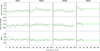 |
Fig. 1. Top and middle panels: coadded FPMA and FPMB light curves shown in the 3–10 keV and 10–79 keV energy bands, respectively. For the various pointings, the ratios between the 10–79 keV light curves and those computed in the 3–10 keV band are shown. The adopted time binning is 4 ks for all the observations. Solid green lines account for the average count rates within each pointing. The exposures in the graph are twice as long as those reported in Table 1 because half of the NuSTAR time is cut due to Earth occultations. |
The normalised excess variance  (e.g. Nandra et al. 1997a; Turner et al. 1999; Vaughan et al. 2003; Ponti et al. 2012) provides a quantitative estimate of the AGN X-ray variability. This estimator can be defined as
 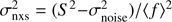 , where f is the unweighted arithmetic mean flux for all the N observations, S represents the variance of the flux as observed, while the mean square uncertainties of the fluxes are accounted for by
  .
.
Following this formula and computing the associated error to  using Eq. (A.1) by Ponti et al. (2012), we computed the
  in the 3–10 keV for all the observations in 10 ks time bins, obtaining an upper limit of
  . Short-term variability has been found to be tightly correlated with the BH mass by many authors (e.g. Nandra et al. 1997b; Vaughan et al. 2003; McHardy et al. 2006; Ponti et al. 2012); therefore, adopting the relation in Ponti et al. (2012) for the
  and MBH (see Table 2), we estimated a lower limit for the BH mass MBH > 3 × 10⁶ M⊙, in agreement with the single-epoch measurement by Grupe et al. (2010).
Best-fit values of the parameters for all the models tested in this 3-79 keV band analysis.
4. Spectral analysis
4.1. Phenomenological modelling
As a first step, we try to reproduce the continuum emission of HE 0436-4717 with a power law absorbed by the Galactic hydrogen column (NH = 1 × 1020 cm−2, Kalberla et al. 2005). In the fit, the photon index and the normalisation are free to vary between the various pointings. To account for the intercalibration of modules A and B, we use a constant set to unity for FPMA and free to vary for FPMB. The two modules are found to be in good agreement (≤3%). This simple model leads to a good fit ( χ2 = 460 for 452 d.o.f.) but some residuals around 6.4 keV and at energies greater than ∼30 keV are still present, suggesting the existence of reprocessed components (see Fig. 2). Therefore, we added a Gaussian component to account for the residuals between 6–7 keV (see Fig. 2), obtaining the following model: const. × phabs × (po + zgauss). The power law shapes the primary continuum, while the zgauss accounts for the presence of neutral or ionised emission lines. The photon index and the normalisation between the different observations are untied and free to vary. For the Gaussian component, we let free to vary and untied among the pointings its energy, intrinsic width (σ), and normalisation. The energy of the Gaussian component is not well constrained since it is 6.50 ± 0.15 keV. Therefore in the subsequent modelling we fix it at 6.4 keV, as for the neutral Fe kα. In a similar fashion, the line width is found consistent with being zero in all the observations with a corresponding upper limit of 400 eV. Thus, in the forthcoming, we set its value to zero. This procedure yielded a best-fit χ2 = 432 for 448 degree of freedom (d.o.f.) and the corresponding best-fit values for the parameters are reported in Table 2. When we fit all the observations together, letting free to vary only the line normalisation, a Δχ2 = 23 for 4 d.o.f. less is found. The presence of this component is then supported by the F-test2 according to which its significance is > 99.9%. The emission line is formally detected in three out of four observations, but its flux is consistent with being constant between all the pointings. The average Fe kα flux is 5.5 ± 3.8 ×10⁻⁶ ph cm−2 s−1, with a corresponding equivalent width of 100 ± 10 eV. We also tested for the presence of a broad component of the line in our spectra. However, this additional broad feature is not required in terms of statistics, with a negligible Δχ2 improvement, and its normalisation is consistent with being zero in all the observations.
 |
Fig. 2. Comparison of the data (black) and power law model (red). An excess of photons is observed between 6.4 and 7 keV suggesting the presence of emission features ascribable to neutral and/or possibly ionized iron. Also a bump of unmodelled photons is found above ∼10 keV. For plotting purposes the FPMA and FPMB spectra of all the epochs and their residuals in terms of errors with respect to the model are displayed grouped (setplot group in Xspec). |
The primary photon index is found to be constant among the different pointings, while weak variability is observed in the primary continuum normalisation. The unmodelled photons above 10 keV in Fig. 2 indicate that part of the emission of HE 0436-4717 is due to reflection of the primary continuum, thus we replace in our best-fit model the power law with pexrav (Magdziarz & Zdziarski 1995). In this new model (const. × phabs × (pexrav + zgauss)), pexrav reproduces the power-law-like primary continuum with its associated reflected component, while the Gaussian line accounts for the Fe Kα. In the fitting procedure the iron abundance is frozen to solar value for all the observations, while the photon index, the normalisation and the reflection fraction are free to vary between the pointings. We also let the high energy cut-off free to vary and untied among the observations. The adoption of this model yields a best-fit of χ 2 = 404 for 440 d.o.f., for which we report the best-fit values in Table 2, second panel.
Allowing for a reflection hump, we find that the photon index is compatible with being constant, and its best-fit values appear steeper than those previously obtained using a simple power law. Within the errors, the reflection fraction is constant between the pointings, and the pexrav normalisation exhibits modest variations. For the high energy cut-off, only lower limits are found (see second panel in Table 2). We further test the reflected Compton component using the following model: const. × phabs × cutoffpl + pexrav). The cut-off power law (cutoffpl) models the primary continuum, while pexrav shapes the reflected component only. The photon index and high energy cut-off are tied between the components and free to vary. Both the primary and reflected component normalisations are free to vary and untied. This model yields a best fit of χ 2 = 406 for 447 d.o.f., and the best-fit parameters are equivalent within the errors with those in the second panel of Table 2. We therefore fit the NuSTAR data tying the normalisation of the reflected component between the observations. The obtained fit (χ 2 = 410 for 450 d.o.f.) is statistically equivalent to the previous one, thus a constant normalisation of the reflected component is found, Nrefl = 1.5 ± 0.5 × 10⁻³ ph keV−1 cm−2 s−1 with a corresponding constant flux F 20−40 keV = 2.6 × 10⁻¹² erg cm−2 s−1.
4.2. Physical modelling
The narrow and constant Fe Kα suggests that the origin of the reprocessed emission of HE 0436-4717 is far from the central BH. However, the geometrical configuration of the reflecting material is unknown. We then tested few models to account for different geometries. At first we tried to reproduce the data set adopting pexmon (Nandra et al. 2007).
Pexmon combines pexrav with self-consistently generated Fe and Ni emission lines. To fit the data with pexmon we adopt the same procedure used for testing pexrav, thus we let free to vary and untied between the observations the photon index, the high energy cut-off, the reflection fraction, and the normalisation. Moreover, we fit the iron abundance AFe tying it between the pointings. The obtained best fit ( χ
2 = 407 for 444 d.o.f.) is statistically equivalent to the one in which pexrav was adopted, and the best-fit values of the parameters are compatible with each other (see Table 2, third panel). Adopting this model that self-consistently accounts for the fluorescence emission lines, we estimate the iron abundance to be  .
.
As an additional test, we have fitted our data set adopting MYTORUS (Yaqoob 2012). Through this model we further test the origin of the HE 0436-4717 reprocessed emission. In fact, MYTORUS accounts for a narrow Fe Kα and its accompanying reflection component by a Compton-thick toroidal material. We assumed a power-law-like illuminating continuum. Both the Γ and normalisation of the primary emission are free to vary and untied between the pointings. At first, we used the MYTORUS tables, accounting for the emission lines and scattering being untied and free to vary. However, the two table normalisations were consistent with each other. Thus we kept them tied together accordingly with the coupled reprocessor solution (Yaqoob 2012). Then, for each observation, we tied the underlying continuum Γ with the one characterising the reflected emission. Finally, we performed the fit, tying the normalisations of the primary continuum and reprocessed component and adding a further constant to account for their mutual weights. This procedure leads to a best fit characterized by χ 2 = 404 for 444 d.o.f., and in the fourth panel of Table 2 we report the corresponding best-fit values. We notice that the constant accounting for the relative normalisations of the primary emission and reflected one (NmyTorus/Npo) has fairly high values. These may suggest a larger covering factor with respect to the default one in MYTORUS. However, the interpretation of this constant is not trivial since it embodies different degenerate information about the chemical abundances and the covering factor itself (see Yaqoob 2012). Moreover, from the fit, only lower limits are obtained for the column density of the reflectors (1.6−2.4 × 1024 cm−2).
Finally we tested Xillver (García & Kallman 2010; García et al. 2013), a model that reproduces the primary continuum and reflection off an accretion disc. Xillver assumes a cut-off power law for the primary emission, and it is commonly used to model reflection from distant material (e.g. Parker et al. 2016). We performed the fit letting free to vary the photon index, the reflection fraction, the normalisation, and the high energy cut-off for each observation. The iron abundance was free to vary but tied between the observations. At first we also fitted the ionisation parameter ξ, but since no improvements were found during the fitting procedure, we fixed its value to the lowest allowed by the model (logξ = 0), close to neutral matter. The obtained best-fit parameters can be found in the fifth panel of Table 2, while the best-fit model for all the observations is shown in Fig. 3.
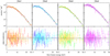 |
Fig. 3. Best-fit model const. × phabs × xillver to the NuSTAR data displayed for each observation. In the x-axis the energy is reported in keV and different colours are used to represent the NuSTAR module A and B spectra. |
As found when adopting pexmon, the photon index is compatible with being constant, and, similarly, the iron abundance is found to be  . Besides a marginally variable underlying continuum, most of the components have a constant behaviour, thus we try to fit the data tying the photon index and the high energy cut-off between the various pointings. The reflection fraction and normalisation of the primary continuum are untied and free to vary between the observations. Following this procedure we obtained a best fit statistically equivalent with the one just discussed ( χ2 = 406 for 449 d.o.f. versus χ2 = 404 for 443 d.o.f.). The best-fit value for the photon index is Γ = 2.01 ± 0.08, while the obtained lower limit for the high energy cut-off is Ecut > 280 keV. We therefore tried to better constrain the reflection fraction R, letting its value free to vary but tied between the observations. This procedure does not change the quality of the fit, but allows us to estimate the averaged value of the reflection fraction to be
  . We then compute the contour plots for the parameters that are shown in Fig. 4.
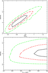 |
Fig. 4. The 68%, 90% and 99% contours in black, red, green respectively computed adopting const. × phabs × xillver. Top panel: photon index and reflection fraction. Bottom panel: contours for the photon index and the high energy cut-off. |
Comptonization is widely accepted to be the origin of the X-ray emission in AGN, therefore, substituting xillver with xillvercp (García & Kallman 2010; García et al. 2013), we tried to investigate the physical properties of the HE0436-4717 hot corona. This model differs from xillver because the primary continuum is shaped by thermal Comptonization through the nthcomp model (Zdziarski et al. 1996). We perform the fit, tying the parameters between the observations, and we let free to vary only the temperature of the hot electrons. In terms of statistics, this fit ( χ 2= for 405 d.o.f. 443) is compatible with the previous one in which xillver was adopted. For the sake of simplicity, in the panel referring to xillver in Table 2 we only report the obtained values for the hot electron temperature kTe, as the other parameters are compatible with those already obtained using xillver within error bars. Furthermore, assuming a spherical geometry and using the nthcomp internal routine for the Thomson optical depth τe, we obtained upper limits for the coronal optical depth of He 0437-4717. These upper limits are reported in the fifth panel of Table 2. Moreover, we fit again the data tying the kTe between the observations ( χ2= for 408 d.o.f. 452). This procedure leads to a lower limit for the corona temperature: kTe > 65 keV. Again, under the assumption of a spherical Comptonizing medium, we computed a corresponding optical depth τe < 1.3. Even though the analysed NuSTAR data did not require any relativistic component, this feature seems to be needed by the XMM-Newton data. Thus we have tested for the presence of a broader and relativistic component adding relxill to our best-fit model. Since the parameters are not well constrained, we set relxill according to the values reported by Bonson et al. (2015): Γ = 2.14, R in = 1.8 rg, AFe = 0.36, inclination θ = 43∘. However, adding relxill yields a fit of χ2 = 406 for 445 d.o.f., thus, on a statistical basis, these NuSTAR data do not require a relativistic component.
5. Discussion
The NuSTAR high sensitivity above 10 keV makes it suitable for investigating the physical conditions of AGN coronae. However, the lack of sufficient statistics limits comparative studies concerning the AGN coronal region. In fact, at present, the largest sample of these sources analysed taking advantage of NuSTAR data counts a few AGN only (< 20; e.g. Fabian et al. 2017; Tortosa et al. 2018). In this framework, the analysis of these multi-epoch NuSTAR observations adds information about the coronal parameter of this particular Seyfert galaxy, enlarging at the same time the number of AGN analysed thanks to NuSTAR.
The 3–79 keV HE 0436-4717 NuSTAR spectra are found to be consistent with being the superposition of two spectral components, a persistent and weakly variable primary emission and a narrow iron Kα with its associated distant reflection continuum. The primary continuum can be described by a power law with photon index Γ = 2.01 ± 0.08 and a lower limit Ec > 280 keV for the cut-off energy. Moreover, a neutral Fe Kα emission line is present in three out of observations and it is found to be narrow. The reflected component is found to be compatible with being constant in flux, and the high energy emission of HE 0436-4717 is in agreement with a scenario in which this reprocessed emission arises from neutral material far from the central engine. Therefore, we have tested a few models that account for different geometrical scenarios. Disc reflection provides a good fit to the data, and, similarly, reprocessed emission by toroidal matter with NH ≳ 2 × 1024 cm−2 is statistically supported.
The NuSTAR data analysed in this work do not require a broad line, consistent with Wang et al. (1998) who found the line to be narrow and likely due to distant reflection. However, XMM-Newton data requires a broad component (Bonson et al. 2015). This discrepancy can be ascribed to the poorer spectral resolution of NuSTAR with respect to XMM-Newton, since part of the broad component flux might be absorbed by the narrower feature. Moreover, we are further limited in testing a complete blurred reflection scenario because any soft excess would occur outside the NuSTAR operating band. Adopting different models, the source iron abundance is found within the errors compatible with being solar ( ). HE 0436-4717 shows modest flux variations within each observation while the average of the counts exhibits a more constant behaviour between the NuSTAR pointings. The largest flux variations are measured on timescales shorter than a day. Past flux measurements in the 2–10 keV band performed using ASCA and XMM-Newton data (Wang et al. 1998; Bonson et al. 2015, respectively) are compatible (3.3−4.6 × 10⁻¹² erg cm−2 s−1) with the flux observed during the NuSTAR pointings. We estimated the 2–10 keV luminosity to be L2−10 keV = 3 ± 0.5 × 1043 erg s−1. Adopting the proper bolometric correction from Marconi et al. (2004), we found the bolometric luminosity of HE 0436-4717 to be Lbol = 7 × 1044 erg s−1. Considering a MBH = 5.9 × 10⁷ M⊙ (Grupe et al. 2010), HE 0436-4717 has an Eddington ratio of L/L
Edd ∼ 0.09.
). HE 0436-4717 shows modest flux variations within each observation while the average of the counts exhibits a more constant behaviour between the NuSTAR pointings. The largest flux variations are measured on timescales shorter than a day. Past flux measurements in the 2–10 keV band performed using ASCA and XMM-Newton data (Wang et al. 1998; Bonson et al. 2015, respectively) are compatible (3.3−4.6 × 10⁻¹² erg cm−2 s−1) with the flux observed during the NuSTAR pointings. We estimated the 2–10 keV luminosity to be L2−10 keV = 3 ± 0.5 × 1043 erg s−1. Adopting the proper bolometric correction from Marconi et al. (2004), we found the bolometric luminosity of HE 0436-4717 to be Lbol = 7 × 1044 erg s−1. Considering a MBH = 5.9 × 10⁷ M⊙ (Grupe et al. 2010), HE 0436-4717 has an Eddington ratio of L/L
Edd ∼ 0.09.
This spectral analysis reveals that HE 0436-4717 did not experience any spectral variation, and this is compatible with what was found in previous works. In fact, Wang et al. (1998) measured a photon index of Γ = 2.15 ± 0.04, while Bonson et al. (2015) obtained Γ = 2.12 ± 0.02. Our NuSTAR measurements are compatible with previous estimates, thus no evidence for long-term spectral variability is found.
The adoption of realististic models including Comptonization allowed us to study the coronal physics of different AGN (e.g. Petrucci et al. 2013; Middei et al. 2018; Ursini et al. 2018), thus we included in our analysis nthcomp to investigate the coronal properties of HE 0436-4717. Accounting for Comptonization and tying the electrons temperature between the various pointings, a lower limit for the coronal temperature is found: kTe > 65 keV. From this value, we derived an upper limit for the electron optical depth of τe < 1.3. Our values for the τe and kTe are in agreement with what is expected for an optically thin and hot medium responsible for the AGN hard X-ray emission. Tortosa et al. (2018) present results on the hot corona parameters of 19 AGN measured with NuSTAR and, in particular, the authors discuss various relations between phenomenological parameters and physical ones. The HE 0436-4717 τe and kTe values are in perfect agreement with the strong anti-correlation they found for the optical depth and the coronal temperature of the 19 Seyfert galaxies.
Moreover, the estimated temperature kTe can be used to investigate how HE 0436-4717 behaves on the compactness-temperature diagram (Fabian et al. 2015, 2017, and references therein). These two parameters are defined as: Θe = kTe/mec2 and 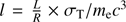 . The first equation accounts for the coronal electron temperature normalised by the rest-frame energy of the electrons, while the second one is used to define the dimensionless compactness parameter (Fabian et al. 2015). In this latter formula, L is the luminosity and R is the radius of coronal (assumed to be spherical). For HE 0436-4717, Θe > 0.13 is obtained. Following Fabian et al. (2015), we computed the luminosity extrapolating its value to the 0.1–200 keV band, L = 1.4 × 1044. Since R is not measured, we assume a value of 10 rg. We then compute the compactness of HE 0436-4717 to be l = 230 (R10)−1, where R10 is just the ratio between the radius and 10 rg. In the Θe − l diagram by Fabian et al. (2015), HE 0436-4717 lies, as does the bulk of the sample analysed by the authors, below the forbidden runaway pair production line. This supports the theory that AGN coronae are hot and radiatively compact. The flux of the reflected component is found to be constant between the observations, and a corresponding averaged reflection fraction
  is obtained. This latter value is compatible with the bulk of the measurements commonly found for Seyfert galaxies (e.g. Perola et al. 2002; Ricci et al. 2017).
6. Summary
This paper focuses on the spectral properties of the Seyfert galaxy HE 0436-4717, and it is based on the analysis of four serendipitous NuSTAR observations performed from December 2014 to December 2015. The main results of this analysis are:
-
Modest flux variability is observed within the various NuSTAR observations on timescales of a few kilo seconds. The average count rate of each epoch in the 3–10 and 10–79 keV bands is only weakly variable. Moreover, we have quantified the source variability, computing the normalised excess variance for this source. We obtained an upper limit for this estimator, σNXS < 0.05. We then converted this value into a lower limit for the BH mass obtaining MBH > 3 × 10⁶ M⊙, in agreement with the single epoch measure by Grupe et al. (2010).
-
A power-law-like spectrum with a corresponding Γ = 2.01 ± 0.08 is found to phenomenologically describe the high energy emission of HE 0436-4717. Between the different observations, the photon index is consistent with being constant, and a lower limit Ecut−off > 280 keV is obtained. We tested a few Comptonization models, obtaining a lower limit of kTe > 65 keV for the hot corona temperature. This temperature allowed us to estimate the optical depth for the HE 0436-4717 hot corona τe < 1.3.
-
A narrow and constant Fe Kα emission line is observed, while a broader component is not required by these data. Both the line and the associated Compton reflection component are in agreement with a scenario in which they arise from Compton-thick matter located far away from the central BH.
NuSTARDAS software guide, Perri et al. (2013), https://heasarc.gsfc.nasa.gov/docs/nustar/analysis/nustar_swguide.pdf
To reliably assess the Fe Kα significance via the F-test, we allowed its normalisation to be negative and positive, as discussed by Protassov et al. (2002).
Acknowledgments
We are grateful to the referee whose comments improved the quality of this work. This work is based on observations obtained with: the NuSTAR mission, a project led by the California Institute of Technology, managed by the Jet Propulsion Laboratory and funded by NASA; XMM-Newton, an ESA science mission with instruments and contributions directly funded by ESA Member States and the USA (NASA). This research has made use of data, software and/or web tools obtained from NASA’s High Energy Astrophysics Science Archive Research Center (HEASARC), a service of Goddard Space Flight Center and the Smithsonian Astrophysical Observatory. Part of this work is based on archival data, software or online services provided by the Space Science Data Center – ASI. SB, RM and FV acknowledge financial support from ASI under grants ASI-INAF I/037/12/0 and n. 2017-14-H.O. F.T. acknowledges support by the Programma per Giovani Ricercatori – anno 2014 “Rita Levi Montalcini”. AM acknowledges financial support from the Italian Space Agency under grant ASI/INAF I/037/12/0-011/13.
References
- Arnaud, K. A. 1996, in Astronomical Data Analysis Software and Systems V, eds. G. H. Jacoby, & J. Barnes, ASP Conf. Ser., 101, 17 [NASA ADS] [Google Scholar]
- Barstow, M. A., & Holberg, J. B. 2003, Extreme Ultraviolet Astronomy, 408 [CrossRef] [Google Scholar]
- Bianchi, S., Guainazzi, M., Matt, G., & Fonseca Bonilla, N. 2007, A&A, 467, L19 [NASA ADS] [CrossRef] [EDP Sciences] [Google Scholar]
- Bianchi, S., Guainazzi, M., Matt, G., Fonseca Bonilla, N., & Ponti, G. 2009, A&A, 495, 421 [NASA ADS] [CrossRef] [EDP Sciences] [Google Scholar]
- Bonson, K., Gallo, L. C., & Vasudevan, R. 2015, MNRAS, 450, 857 [NASA ADS] [CrossRef] [Google Scholar]
- Cappi, M., Panessa, F., Bassani, L., et al. 2006, A&A, 446, 459 [NASA ADS] [CrossRef] [EDP Sciences] [Google Scholar]
- De Rosa, A., Fabian, A. C., & Piro, L. 2002, MNRAS, 334, L21 [NASA ADS] [CrossRef] [Google Scholar]
- Fabian, A. C., Rees, M. J., Stella, L., & White, N. E. 1989, MNRAS, 238, 729 [NASA ADS] [CrossRef] [Google Scholar]
- Fabian, A. C., Lohfink, A., Kara, E., et al. 2015, MNRAS, 451, 4375 [NASA ADS] [CrossRef] [Google Scholar]
- Fabian, A. C., Lohfink, A., Belmont, R., Malzac, J., & Coppi, P. 2017, MNRAS, 467, 2566 [NASA ADS] [CrossRef] [Google Scholar]
- García, J., & Kallman, T. R. 2010, ApJ, 718, 695 [NASA ADS] [CrossRef] [Google Scholar]
- García, J., Dauser, T., Reynolds, C. S., et al. 2013, ApJ, 768, 146 [NASA ADS] [CrossRef] [Google Scholar]
- George, I. M., & Fabian, A. C. 1991, MNRAS, 249, 352 [NASA ADS] [CrossRef] [Google Scholar]
- Grupe, D., Komossa, S., Leighly, K. M., & Page, K. L. 2010, ApJS, 187, 64 [NASA ADS] [CrossRef] [Google Scholar]
- Guillot, S., Kaspi, V. M., Archibald, R. F., et al. 2016, MNRAS, 463, 2612 [NASA ADS] [CrossRef] [Google Scholar]
- Haardt, F., & Maraschi, L. 1991, ApJ, 380, L51 [NASA ADS] [CrossRef] [Google Scholar]
- Haardt, F., & Maraschi, L. 1993, ApJ, 413, 507 [NASA ADS] [CrossRef] [MathSciNet] [Google Scholar]
- Haardt, F., Maraschi, L., & Ghisellini, G. 1994, ApJ, 432, L95 [NASA ADS] [CrossRef] [Google Scholar]
- Halpern, J. P., & Marshall, H. L. 1996, ApJ, 464, 760 [NASA ADS] [CrossRef] [Google Scholar]
- Halpern, J. P., Leighly, K. M., & Marshall, H. L. 2003, ApJ, 585, 665 [NASA ADS] [CrossRef] [Google Scholar]
- Harrison, F. A., Craig, W. W., Christensen, F. E., et al. 2013, ApJ, 770, 103 [NASA ADS] [CrossRef] [Google Scholar]
- Kalberla, P. M. W., Burton, W. B., Hartmann, D., et al. 2005, A&A, 440, 775 [NASA ADS] [CrossRef] [EDP Sciences] [Google Scholar]
- Lansbury, G. B., Alexander, D. M., Aird, J., et al. 2017, ApJ, 846, 20 [NASA ADS] [CrossRef] [Google Scholar]
- Leighly, K. M. 2005, Ap&SS, 300, 137 [NASA ADS] [CrossRef] [Google Scholar]
- Magdziarz, P., & Zdziarski, A. A. 1995, MNRAS, 273, 837 [NASA ADS] [CrossRef] [Google Scholar]
- Marconi, A., Risaliti, G., Gilli, R., et al. 2004, MNRAS, 351, 169 [NASA ADS] [CrossRef] [Google Scholar]
- Matt, G., Perola, G. C., & Piro, L. 1991, A&A, 247, 25 [NASA ADS] [Google Scholar]
- McHardy, I. M., Koerding, E., Knigge, C., Uttley, P., & Fender, R. P. 2006, Nature, 444, 730 [NASA ADS] [CrossRef] [PubMed] [Google Scholar]
- Middei, R., Vagnetti, F., Bianchi, S., et al. 2017, A&A, 599, A82 [NASA ADS] [CrossRef] [EDP Sciences] [Google Scholar]
- Middei, R., Bianchi, S., Cappi, M., et al. 2018, A&A, 615, A163 [NASA ADS] [CrossRef] [EDP Sciences] [Google Scholar]
- Nandra, K., George, I. M., Mushotzky, R. F., Turner, T. J., & Yaqoob, T. 1997a, ApJ, 476, 70 [NASA ADS] [CrossRef] [Google Scholar]
- Nandra, K., George, I. M., Mushotzky, R. F., Turner, T. J., & Yaqoob, T. 1997b, ApJ, 477, 602 [NASA ADS] [CrossRef] [Google Scholar]
- Nandra, K., O’Neill, P. M., George, I. M., & Reeves, J. N. 2007, MNRAS, 382, 194 [NASA ADS] [CrossRef] [Google Scholar]
- Nicastro, F., Piro, L., De Rosa, A., et al. 2000, ApJ, 536, 718 [NASA ADS] [CrossRef] [Google Scholar]
- Parker, M. L., Komossa, S., Kollatschny, W., et al. 2016, MNRAS, 461, 1927 [NASA ADS] [CrossRef] [Google Scholar]
- Perola, G. C., Matt, G., Fiore, F., et al. 2000, A&A, 358, 117 [NASA ADS] [Google Scholar]
- Perola, G. C., Matt, G., Cappi, M., et al. 2002, A&A, 389, 802 [NASA ADS] [CrossRef] [EDP Sciences] [Google Scholar]
- Perri, M., Puccetti, S., Spagnuolo, N., et al. 2013, The NuSTAR Data Analysis Software Guide, https://heasarc.gsfc.nasa.gov/docs/nustar/analysis/nustar_swguide.pdf [Google Scholar]
- Petrucci, P.-O., Paltani, S., Malzac, J., et al. 2013, A&A, 549, A73 [NASA ADS] [CrossRef] [EDP Sciences] [Google Scholar]
- Ponti, G., Papadakis, I., Bianchi, S., et al. 2012, A&A, 542, A83 [NASA ADS] [CrossRef] [EDP Sciences] [Google Scholar]
- Protassov, R., van Dyk, D. A., Connors, A., Kashyap, V. L., & Siemiginowska, A. 2002, ApJ, 571, 545 [NASA ADS] [CrossRef] [Google Scholar]
- Reynolds, C. S. 2013, Classical Quantum Gravity, 30, 244004 [NASA ADS] [CrossRef] [Google Scholar]
- Ricci, C., Trakhtenbrot, B., Koss, M. J., et al. 2017, ApJS, 233, 17 [NASA ADS] [CrossRef] [Google Scholar]
- Rybicki, G. B., & Lightman, A. P. 1979, Radiative Processes in Astrophysics (New York: Wiley-Interscience) [Google Scholar]
- Tortosa, A., Bianchi, S., Marinucci, A., Matt, G., & Petrucci, P. O. 2018, A&A, 614, A37 [NASA ADS] [CrossRef] [EDP Sciences] [Google Scholar]
- Turner, T. J., George, I. M., Nandra, K., & Turcan, D. 1999, ApJ, 524, 667 [NASA ADS] [CrossRef] [Google Scholar]
- Ursini, F., Petrucci, P. O., Matt, G., et al. 2018, MNRAS, 478, 2663 [NASA ADS] [CrossRef] [Google Scholar]
- Vagnetti, F., Turriziani, S., & Trevese, D. 2011, A&A, 536, A84 [NASA ADS] [CrossRef] [EDP Sciences] [Google Scholar]
- Vagnetti, F., Middei, R., Antonucci, M., Paolillo, M., & Serafinelli, R. 2016, A&A, 593, A55 [NASA ADS] [CrossRef] [EDP Sciences] [Google Scholar]
- Vaughan, S., Edelson, R., Warwick, R. S., & Uttley, P. 2003, MNRAS, 345, 1271 [NASA ADS] [CrossRef] [Google Scholar]
- Véron-Cetty, M.-P., & Véron, P. 2006, A&A, 455, 773 [NASA ADS] [CrossRef] [EDP Sciences] [Google Scholar]
- Wang, T., Otani, C., Matsuoka, M., et al. 1998, MNRAS, 293, 397 [NASA ADS] [CrossRef] [Google Scholar]
- Wisotzki, L., Christlieb, N., Bade, N., et al. 2000, A&A, 358, 77 [NASA ADS] [Google Scholar]
- Yaqoob, T. 2012, MNRAS, 423, 3360 [NASA ADS] [CrossRef] [Google Scholar]
- Zdziarski, A. A., Johnson, W. N., & Magdziarz, P. 1996, MNRAS, 283, 193 [NASA ADS] [CrossRef] [Google Scholar]
- Zheng, X. C., Xue, Y. Q., Brandt, W. N., et al. 2017, ApJ, 849, 127 [NASA ADS] [CrossRef] [Google Scholar]
All Tables
Observation ID, start date and net exposure time in kiloseconds for the NuSTAR serendipitous observations analysed in this paper.
Best-fit values of the parameters for all the models tested in this 3-79 keV band analysis.
All Figures
|
Fig. 1. Top and middle panels: coadded FPMA and FPMB light curves shown in the 3–10 keV and 10–79 keV energy bands, respectively. For the various pointings, the ratios between the 10–79 keV light curves and those computed in the 3–10 keV band are shown. The adopted time binning is 4 ks for all the observations. Solid green lines account for the average count rates within each pointing. The exposures in the graph are twice as long as those reported in Table 1 because half of the NuSTAR time is cut due to Earth occultations. |
| In the text | |
|
Fig. 2. Comparison of the data (black) and power law model (red). An excess of photons is observed between 6.4 and 7 keV suggesting the presence of emission features ascribable to neutral and/or possibly ionized iron. Also a bump of unmodelled photons is found above ∼10 keV. For plotting purposes the FPMA and FPMB spectra of all the epochs and their residuals in terms of errors with respect to the model are displayed grouped (setplot group in Xspec). |
| In the text | |
|
Fig. 3. Best-fit model const. × phabs × xillver to the NuSTAR data displayed for each observation. In the x-axis the energy is reported in keV and different colours are used to represent the NuSTAR module A and B spectra. |
| In the text | |
|
Fig. 4. The 68%, 90% and 99% contours in black, red, green respectively computed adopting const. × phabs × xillver. Top panel: photon index and reflection fraction. Bottom panel: contours for the photon index and the high energy cut-off. |
| In the text | |
Current usage metrics show cumulative count of Article Views (full-text article views including HTML views, PDF and ePub downloads, according to the available data) and Abstracts Views on Vision4Press platform.
Data correspond to usage on the plateform after 2015. The current usage metrics is available 48-96 hours after online publication and is updated daily on week days.
Initial download of the metrics may take a while.