| Issue |
A&A
Volume 618, October 2018
|
|
|---|---|---|
| Article Number | A117 | |
| Number of page(s) | 6 | |
| Section | Astronomical instrumentation | |
| DOI | https://doi.org/10.1051/0004-6361/201833090 | |
| Published online | 17 October 2018 | |
Fused CLEAN deconvolution for compact and diffuse emission
1
Guizhou University, Guiyang, 550025 PR China
e-mail: This email address is being protected from spambots. You need JavaScript enabled to view it.
2
CAS Key Laboratory of Solar Activity, National Astronomical Observatories, Beijing, 100012 PR China
Received:
24
March
2018
Accepted:
20
July
2018
Abstract
Context. CLEAN algorithms are excellent deconvolution solvers that remove the sidelobes of the dirty beam to clean the dirty image. From the point of view of the scale, there are two types: scale-insensitive CLEAN algorithms, and scale-sensitive CLEAN algorithms. Scale-insensitive CLEAN algorithms perform excellently well for compact emission and perform poorly for diffuse emission, while scale-sensitive CLEAN algorithms are good for both point-like emission and diffuse emission but are often computationally expensive. However, observed images often contain both compact and diffuse emission. An algorithm that can simultaneously process compact and diffuse emission well is therefore required.
Aims. We propose a new deconvolution algorithm by combining a scale-insensitive CLEAN algorithm and a scale-sensitive CLEAN algorithm. The new algorithm combines the advantages of scale-insensitive algorithms for compact emission and scale-sensitive algorithms for diffuse emission. At the same time, it avoids the poor performance of scale-insensitive algorithms for diffuse emission and the great computational load of scale-sensitive algorithms for compact emission in residuals.
Methods. We propose a fuse mechanism to combine two algorithms: the Asp-Clean2016 algorithm, which solves the computationally expensive problem of convolution operation in the fitting procedure, and the classical Högbom CLEAN (Hg-Clean) algorithm, which is faster and works equally well for compact emission. It is called fused CLEAN (fused-Clean) in this paper.
Results. We apply the fused-Clean algorithm to simulated EVLA data and compare it to widely used algorithms: the Hg-Clean algorithm, the multi-scale CLEAN (Ms-Clean), and the Asp-Clean2016 algorithm. The results show that it performs better and is computationally effective.
Key words: methods: data analysis / techniques: image processing
© ESO 2018
1. Introduction
For many reasons, such as technical difficulties, the size of a single dish is severely limited, as is its resolution. Interferometric measurements with some imaging techniques such as deconvolution can go beyond the resolution limitation of a single telescope. Radio telescope arrays currently often use tens of telescopes to measure visibilities. However, the sampling is incomplete. These missing spatial frequencies lead to a dirty image, which is the corrupted version of the true sky image. Deconvolution algorithms are used to remove the effects of the corruption to obtain the restored image.
The most widely used deconvolution algorithms in the radio synthesis imaging field are CLEAN algorithms. Scale-insensitive CLEAN algorithms decompose the true sky image as a collection of point sources or scaled delta functions. The original algorithm (Högbom 1974) has been proposed by Högbom in the 1970s. It is a matched-pursuit algorithm and employs iterations to approximate the true sky image. For point-like emission, it is quite good and speedy enough. However, it needs a huge number of scaled delta functions to approximate diffuse emission and complex images, and it lacks a mechanism to introduce the dependence among the neighboring points. Thus the residuals of extended sources often include some significantly correlated structures.
Scale-sensitive CLEAN algorithms (Bhatnagar & Cornwell 2004; Cornwell 2008) introduce a priori the knowledge that the true image is composed of different spatial scales. The pixels within one scale are dependent, which can constrain the unsampled spatial frequencies. Extended emission can be represented with a small number of components in scale-sensitive CLEAN algorithms. Even though some papers (Zhang et al. 2016a,b) have improved scale-sensitive CLEAN algorithms, they are still not computationally efficient for compact emission.
So far, these deconvolution algorithms are designed for either compact or diffuse emission. However, observations contain both compact and diffuse emission within the field of view, which requires an algorithm that can process both compact and diffuse emission well. To solve the problem, we propose an efficient algorithm that combines Asp-Clean2016 and Hg-Clean. This is not a direct combination of the two algorithms, but a more sophisticated way; it only combines in the phase of the component search in the minor cycle and uses the same major cycle.
The paper is structured as follows. In Sect. 2 we describe the imaging theory, the Hg-Clean algorithm, and the Asp-Clean2016 algorithm. In Sect. 3 we describe the fused-Clean algorithm in detail. In Sect. 4 we give some examples and compare our results to other classical algorithms. In Sect. 5 we discuss this algorithm and conclude.
2. Imaging theory and CLEAN algorithms
To understand our algorithm, here we introduce the radio interferometric imaging theory and two algorithms that are used in the proposed algorithm.
2.1. Imaging theory
In the van Cittert–Zernike theorem (Thompson et al. 2017), the true visibility function and the sky brightness function are a pair of Fourier transformations. The true visibilities are Vtrue
 (1)
(1)
where F is the Fourier transformation and Itrue is the sky brightness function. This is an ideal and continuous case. The true image can be recovered by directly employing inverse Fourier transformation. For real cases, however, the sample is incomplete and noisy. The measured visibilities Vmeasured
 (2)
(2)
where S is the sampling function and N is the noise in Fourier domain. Here we ignore these operations of weighting, convolutional interpolation, and resampling, and express the dirty image Idirty as (3)
(3)
where F−1 is the inverse Fourier transform operation. In the convolution theorem of Fourier transform theory, the dirty image Idirty can be expressed as (4)
(4)
where Bdirty is a Toeplitz matrix that is composed of the shifted dirty beams. Because of the incomplete sampling, the dirty beam often has many non-ignorable wide-spread sidelobes. Deconvolution is a solver that removes the effect of these dirty beam sidelobes.
2.2. Hg-Clean algorithm
The Hg-Clean algorithm decomposes the true sky brightness as a set of scaled delta functions, (5)
(5)
where  is the amplitude of the nth component and δn is the delta function in the position (xn, yn). The error of the component estimation in the minor cycle is corrected in the fused-Clean algorithm by updating residual visibilities from the original visibility data in the major cycle. Very many components are needed to represent a large diffuse emission. However, the computational load of the algorithm for each component is small. This is effective for compact emission.
2.3. Asp-Clean2016 algorithm
The Asp-Clean2016 algorithm (Zhang et al. 2016a) is an efficient implementation of the Asp-Clean algorithm (Bhatnagar & Cornwell 2004). It parameterizes the true sky image as a collection of circular Gaussian functions with different scales, (6)
(6)
where (7)
(7)
where αn is the amplitude of the nth component, σn is the scale of the Gaussian component, and xn and yn are the parameters of positions.
The Asp-Clean algorithm finds the best-fit scale components with active sets by minimizing the objective function χ2 for each component (8)
(8)
where  is the residual image in (n − 1)th iteration,
  is the current model component, and ∥ ⋅ ∥2 is the Euclidean norm. Since the convolution is in the component-fitting objective function, the Asp-Clean algorithm is computationally expensive. It is removed to speed up the process by analytically computing model components in the Asp-Clean2016 algorithm (Zhang et al. 2016a). The procedure of the Asp-Clean2016 algorithm is similar to the Asp-Clean algorithm, but it minimizes a different objective function of the fitting part,
 (9)
(9)
where  is a Gaussian component that was fitted from the residual image. This is very efficient for diffuse emission (Zhang et al. 2016a). However, it is still time-consuming for compact emission.
3. Fused-Clean algorithm
To achieve the goal of simultaneously processing both compact and diffuse emission well, the fused-Clean algorithm combines the advantages of the different algorithms and can automatically trigger different algorithms in different situations to speed up and improve the performance of the algorithm. The basic procedure is as follows.
-
Smooth residual image
 (the dirty image for the first time) with s scales.
 -
Find peaks from these smoothed residual images
 ; the global peak Gl(al,xl,yl,σl) is used as the initial guess of the current parameters.
 -
Trigger an algorithm according to the current situation.
-
Find new parameters of the current model component
 .
. -
Update the model image
 .
. -
Calculate the residual image
 .
. -
Iterate until one of the termination criteria is satisfied.
-
Compute the restored image
 with the restored beam Bclean after m iterations.
All model components are found by equivalently minimizing the objective function in the major cycle, (10)
(10)
It can find the best fit to the measured visibilities.
In the beginning phase of deconvolution, the matched-filtering technique is used to find the initial position and scale of the strongest emission in the same way as in the Asp-Clean2016 algorithm. If the initial scale is larger than the scale of the dirty beam, then the minor cycle of the Asp-Clean2016 algorithm is triggered once. The optimal scale and position are found by explicitly minimizing the objective function, (11)
(11)
where  is a Gaussian function with parameters (amplitude αnb, location xnb, ynb, and width ωnb). The updated direction is estimated by computing the gradient of χ2 with respect to the parameters pnb given by
![Mathematical equation: $ \begin{aligned} \frac{\partial \chi ^{2}}{\partial p_\mathrm{nb}}= \frac{\partial \chi ^{2}}{\partial I^\mathrm{gauss}_\mathrm{nb}}\frac{\partial I^\mathrm{gauss}_\mathrm{nb}}{\partial p_\mathrm{nb}} = -2\left[I_\mathrm{n}^\mathrm{residual}\right]^\mathrm{T}\frac{\partial I^\mathrm{gauss}_\mathrm{nb}}{\partial p_\mathrm{nb}}, \end{aligned} $](/articles/aa/full_html/2018/10/aa33090-18/aa33090-18-eq23.gif) (12)
(12)
where pnb ≡ {αnb, xnb, ynb, ωnb}. For the second-order optimization method (e.g., the Levenberg–Marquardt algorithm Marquardt 1963), we also need to compute or approximate the Hessian matrix. After converging to the solution of  , the parameterized component can be analytically computed as
 (13)
(13)
where ωn, ωnb, ωb are the widths of the current model component  ,
,  and the Gaussian beam approximated from the dirty beam, respectively. The amplitude αn of
  is computed as
 (14)
(14)
where αb and αnb are the amplitudes of the Gaussian beam and  , respectively.
Explicitly, minimization optimizes each component, which is a best fit for the current residuals. The Asp-Clean2016 algorithm (Zhang et al. 2016a) has shown that the analytical computation of components is very efficient for diffuse emission.
When the initial scale estimated by matched-filtering technique is smaller than a threshold (e.g., 1.2 times the width of the dirty beam) or very small scale components frequently appear in the last iterations (e.g., the FWHM of five components are smaller than 1 pixel in the last ten components), then the minor cycle of the Hg-Clean algorithm will be triggered. Compared to scale-sensitive CLEAN algorithms, the Hg-Clean is more efficient for compact emission. It does not perform an explicit fitting, but determines the peak of the current residuals and then subtracts a scaled version of the dirty beam from the current residuals. In other words, the updated direction is estimated by finding the peak of the current residuals,![Mathematical equation: $ \begin{aligned} \frac{\partial \chi ^{2}}{\partial p_\mathrm{n}}\equiv \frac{\partial \chi ^{2}}{\partial I^\mathrm{amp}_\mathrm{n}} = -2\left[I_\mathrm{n}^\mathrm{residual}\right]^\mathrm{T}\frac{\partial p_\mathrm{n}}{\partial I^\mathrm{amp}_\mathrm{n}}=-2I_\mathrm{{n},x_\mathrm{n},{ y}_\mathrm{n}}^\mathrm{residual}, \end{aligned} $](/articles/aa/full_html/2018/10/aa33090-18/aa33090-18-eq31.gif) (15)
(15)
where pn =  and
and  is the peak point located at (xn, yn) in the nth iterations. The iterative search for
  and then the shift-and-subtract operation in the Hg-Clean algorithm is equivalent to a fast implementation of the minimization of the objective function given by Eq. (8). When the Hg-Clean is triggered, it will be ran for several times. In practice, more compact emission will appear in the residuals when the deconvolution reaches deeper, so that a monotonic function for the triggering number can process it well. We have found the following relation to work well:
 (16)ttn is the times of executing Hg-Clean when Hg-Clean is triggered tnth times. The specific form of this function in Eq. (16) is not important, but with the increase of the triggering times for the Hg-Clean algorithm, the function should be increasing.
In the fused-Clean algorithm, the Hg-Clean algorithm is used for compact emission and the Asp-Clean2016 algorithm is used for diffuse emission. The scale adaptivity of the Asp-Clean2016 algorithm can separate emission and noise, while the Hg-Clean algorithm is efficient for compact emission. In the fused-Clean algorithm, the two algorithms are triggered alternately, so that emission and noise are effectively separated.
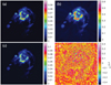 |
Fig. 1. Results of simulated EVLA observations of the M 31 image deconvolved by the fused-Clean algorithm. Panel a: original image; panel b: dirty image with Briggs weighting; panel c: model image; and panel d: residual image. |
4. Numerical experiment and comparison
In this section, we apply the fused-Clean algorithm to the EVLA1 simulated data to evaluate its performance and compare it to these frequently used CLEAN algorithms: the Hg-Clean algorithm, the Ms-Clean algorithm, and the Asp-Clean2016 algorithm. The test M 31 image is shown in Fig. 1a, and its brightness ranges from 0 Jy pixel−1 to 0.1 Jy pixel−1. We performed a simulated observation with the B configuration of EVLA using the CASA software2. The observation was made in L band with a bandwidth of 1 GHz and 32 channels, and it lasted six hours. Gaussian white noise was added to the “measured” visibilities, which means that the dirty image has a noise level of RMS 5 × 10⁻⁵ Jy. The resolution of the images was 1″ and the width of the main lobe of the dirty beam was about 2″. The corresponding dirty image with the robust (=0) weighting is shown in Fig. 1b, where the data range reaches from −0.039 Jy pixel−1 to 0.61 Jy pixel−1.
The deconvolution results are shown in Fig. 1. The model image displayed in Fig. 1c is composed of 155 extended components and 20 196 compact components, which can represent the true emission well. No significant signal in the residual image displayed in Fig. 1d indicates that the fused-Clean deconvolution can extract the signal fully, and signal and noise are effectively separated.
These scale choices of deconvolving the M 31 image and the change of the model flux with iterations are displayed in Fig. 2, which contains only the first 100 iterations and the last 10 000 iterations for effective visualization. The choices of algorithms can be known through the choices of the component scale sizes. If the scale size is greater than zero, then the Asp-Clean2016 algorithm is selected; otherwise the Hg-Clean algorithm is selected. We can know the deconvolution behaviors of the fused-Clean algorithm from Fig. 2. 1) Most flux was recovered in the beginning phase of the deconvolution. The main emission is reconstructed in the first ∼50 iterations. Asp-Clean2016 is more frequently executed in the beginning phase because Asp-Clean2016 has more sparse representation capacity for diffuse emission. 2) Most iterations were used to reconstruct weak and small-scale emission. This compact emission corresponds to compact sources or broken emission from an inaccurate representation of diffuse emission. Hg-Clean is required frequently to deconvolve this compact emission to approximate the latent true image. 3) After triggering the Hg-Clean algorithm, some weak and large-scale emission may appear and can be reconstructed effectively by the Asp-Clean2016 algorithm. 4) We did not set the iteration number for the Asp-Clean2016 and Hg-Clean algorithms. The 155 Asp-Clean2016 and 20 196 Hg-Clean deconvolutions are completely determined by the scale complexity of the dirty image and by the parameters of the deconvolution algorithm. This also shows the adaptive capacity of calling these two sub-algorithms.
In short, diffuse emission is recovered with the Asp-Clean2016 algorithm, and compact emission is reconstructed with the Hg-Clean algorithm. The Asp-Clean2016 algorithm is almost always used preferentially when the residual image contains much signal. As the deconvolution continues, the signals in the residual image will decrease and much scale-less emission will appear. Then the Hg-Clean algorithm dominates the deconvolution process.
To compare the performance of the fused-Clean algorithm with other typical CLEAN deconvolution algorithms, the corresponding deconvolution results are displayed in Fig. 3 and listed in Table 1. The model images displayed in Fig. 3a0 from the Hg-Clean algorithm are composed of 100 000 compact components, and the corresponding residual image in Fig. 3a1 contains many correlated features because delta function cannot physically represent diffuse emission well. The model image from the Ms-Clean algorithm that uses enumeration scales has 2000 components and less signal in the residuals. The Asp-Clean2016 and fused-Clean algorithms use adaptive scales. They can represent an image more sparsely than the previous two algorithms. The fused-Clean algorithm combines the Asp-Clean2016 algorithm with the Hg-Clean algorithm, which represents compact emission more effectively. This can separate signal and noise more effectively. No significant signal is in the residual image displayed in Fig. 3d1 from the fused-Clean algorithm. The fused-Clean deconvolution has the highest dynamic range (defined in Li et al. 2011) in this experiment from Table 1. All these results show that the performance of the fused-Clean algorithm is excellent, which can be also proved by the numerical comparison in Table 1.
It is worth mentioning that the fused-Clean algorithm is more robust and faster than the Asp-Clean2016 algorithm. A combination of the Hg-Clean algorithm equivalently introduces a new scheme to jump out of the possible local optimum in the Asp-Clean2016 algorithm. In the M 31 simulation, the fused-Clean deconvolution took about 4 min, which is about four times faster than the Asp-Clean2016 algorithm. Experiments were ran on a typical graphics workstation. The speed increase arises because the Hg-Clean algorithm was used to represent compact emission. In the Asp-Clean2016 algorithm, finding a compact component from the current residual image needs to be explicitly fitted. This is achieved through iterative optimization, which is time consuming. However, finding a compact component through the Hg-Clean algorithm only requires identifying the maximum value in the current residual image and some simple operations.
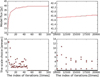 |
Fig. 2. Scale choices and model flux for deconvolving the dirty M 31 image with fused-Clean. |
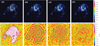 |
Fig. 3. Deconvolution results of the M 31 image. From left to right, columns: Hg-Clean, Ms-Clean, Asp-Clean2016, and fused-Clean. From top to bottom, rows: model images and the residual images. |
Numerical comparison of different deconvolution algorithms for the “M 31” simulation.
5. Discussion and summary
The fused-Clean introduces a good algorithm framework and the thought of algorithm union. In other words, this is a general method that can be applied to more algorithmic combinations than a mere combination of the Hg-Clean aglorithm and the Asp-Clean2016 algorithm. Combined algorithms can combine the advantages of different algorithms without maintaining their disadvantages. It performs excellently well, which is difficult for a single algorithm. In addition, if a combined algorithm can reduce the total computation complexity, then it is very helpful that a deconvolution algorithm can be developed into software. For this purpose, many scale-insensitive and scale-sensitive algorithms can be combined to speed up the deconvolution process. For example, the Ms-Clean (Cornwell 2008) or MTMFS (Rau & Cornwell 2011) can be combined with a scale-insensitive algorithm such as the Clark CLEAN (Clark 1980).
An algorithm combination should consider intrinsic factors and relations of model decomposition among iterations properly. In other words, a combined algorithm should be not a simple mechanical concatenation. A simple mechanical concatenation may not be sufficient to improve the performance.
Compressive-sensing based deconvolution algorithms make the obvious assumption that the signal is sparse in a certain domain. The CLEAN-based algorithm does not make such an assumption. Therefore, the performance of CLEAN-based algorithms (e.g., runtime and fidelity) is more stable when conditions change (see Li et al. 2011). At the same time, the fused-Clean algorithm is naturally applicable to the CLEAN algorithm framework, that is, to minor cycle and major cycle (it is also implemented in the standard minor and major cycles) and also integrates well with some other typical synthesis imaging techniques, such as wide-field corrections.
The minor cycle of the fused-Clean contains the component estimation methods of the Asp-Clean2016 and the Hg-Clean algorithms. The Asp-Clean2016 algorithm employs an analytical way to significantly reduce the computational load and at the same time keeps the excellent performance of adaptive scale deconvolution. The advantage of the Hg-Clean algorithm is that it is excellent and fast for compact emission, but its disadvantage is that it is slow and difficult to fully represent for diffuse emission. The fused-Clean algorithm combines the speed and excellent performance of the Asp-Clean2016 algorithm for diffuse emission with the speed of the Hg-Clean algorithm for compact emission, and it avoids the slow speed of the Asp-Clean2016 algorithm for compact emission and the poor performance for diffuse emission of the Hg-Clean algorithm.
Tests show that the performance of the fused-Clean algorithm is better than these typical CLEAN-based deconvolution algorithms. The algorithm is implemented with the CASA and Python language. The work to build it as an available deconvolution algorithm into the CASA software package is currently ongoing.
Acknowledgments
We thank the people who worked and are working on the Python and CASA projects, which provide an excellent development and simulation environment. The work is supported by the Open Research Program of the CAS Key Laboratory of Solar Activity (KLSA201805) and the Guizhou Science & Technology Cooperation Project–Talent Platform ([2017]5788).
References
- Bhatnagar, S., & Cornwell, T. J. 2004, A&A, 426, 747 [NASA ADS] [CrossRef] [EDP Sciences] [Google Scholar]
- Bhatnagar, S., Rau, U., Green, D. A., & Rupen, M. P. 2011, ApJ, 739, L20 [NASA ADS] [CrossRef] [Google Scholar]
- Clark, B. G. 1980, A&A, 89, 377 [NASA ADS] [Google Scholar]
- Cornwell, T. J. 2008, IEEE J. Sel. Top. Signal Process, 2, 793 [Google Scholar]
- Högbom, J. A. 1974, A&AS, 15, 417 [Google Scholar]
- Li, F., Cornwell, T. J., & de Hoog, F. 2011, A&A, 528, A31 [NASA ADS] [CrossRef] [EDP Sciences] [Google Scholar]
- Marquardt, D. W. 1963, J. Soc. Ind. Appl. Math., 11, 431 [Google Scholar]
- Rau, U., & Cornwell, T. J. 2011, A&A, 532, A71 [NASA ADS] [CrossRef] [EDP Sciences] [Google Scholar]
- Schwab, F. R., & Cotton, W. D. 1983, AJ, 88, 688 [NASA ADS] [CrossRef] [Google Scholar]
- Thompson, A. R., Moran, J. M., & Swenaon, G. W. 2017, Interferometry and Synthesis in Radio Astronomy, 3rd edn. (Switzerland: Springer International Publishing) [Google Scholar]
- Zhang, L., Bhatnagar, S., Rau, U., & Zhang, M. 2016a, A&A, 592, A128 [NASA ADS] [CrossRef] [EDP Sciences] [Google Scholar]
- Zhang, L., Zhang, M., & Liu, X. 2016b, Ap&SS, 361, 153 [NASA ADS] [CrossRef] [Google Scholar]
All Tables
Numerical comparison of different deconvolution algorithms for the “M 31” simulation.
All Figures
|
Fig. 1. Results of simulated EVLA observations of the M 31 image deconvolved by the fused-Clean algorithm. Panel a: original image; panel b: dirty image with Briggs weighting; panel c: model image; and panel d: residual image. |
| In the text | |
|
Fig. 2. Scale choices and model flux for deconvolving the dirty M 31 image with fused-Clean. |
| In the text | |
|
Fig. 3. Deconvolution results of the M 31 image. From left to right, columns: Hg-Clean, Ms-Clean, Asp-Clean2016, and fused-Clean. From top to bottom, rows: model images and the residual images. |
| In the text | |
Current usage metrics show cumulative count of Article Views (full-text article views including HTML views, PDF and ePub downloads, according to the available data) and Abstracts Views on Vision4Press platform.
Data correspond to usage on the plateform after 2015. The current usage metrics is available 48-96 hours after online publication and is updated daily on week days.
Initial download of the metrics may take a while.