| Issue |
A&A
Volume 618, October 2018
|
|
|---|---|---|
| Article Number | A105 | |
| Number of page(s) | 5 | |
| Section | The Sun | |
| DOI | https://doi.org/10.1051/0004-6361/201832609 | |
| Published online | 17 October 2018 | |
Southward shift of the coronal neutral line and the heliospheric current sheet: Evidence for radial evolution of hemispheric asymmetry
ReSoLVE Centre of Excellence, Space Climate research unit, University of Oulu, PO Box 3000, 90014 Oulu, Finland
e-mail: This email address is being protected from spambots. You need JavaScript enabled to view it.
Received:
8
January
2018
Accepted:
3
August
2018
Abstract
Aims. The heliospheric current sheet (HCS) has been observed to be southward shifted in the late declining to minimum phase of the solar cycle. Here we study the existence of a simultaneous shift in the heliosphere and in the corona using a robust new method.
Methods. We use the synoptic maps of the photospheric field of the Wilcox Solar Observatory (WSO) and the Mount Wilson Observatory (MWO) together with the potential field source surface (PFSS) model to calculate the coronal magnetic field and compare it with the simultaneous heliospheric magnetic field of the NASA/NSSDC OMNI 2 dataset. We divide the magnetic field into the two sectors, towards (T) and away (A) from the Sun, and calculate how often the sector polarities at 1 AU and in the corona match each other. We divide the sectors both at 1 AU and in the corona. We also calculate the annual (T − A)/(T + A) ratios of sector occurrence both at 1 AU and in the corona.
Results. We verify that the HCS/neutral line is southward shifted both in the corona and heliosphere. We find that the coronal shift is systematically larger than the simultaneous heliospheric shift.
Conclusions. The fact that the southward shift of the coronal neutral line is larger than the simultaneous shift of the heliospheric current sheet at 1 AU implies that the radial evolution of the magnetic field between the two sites is different between the northern and southern hemispheres.
Key words: Sun: corona / Sun: heliosphere / Sun: magnetic fields
© ESO 2018
1. Introduction
Solar wind is a flow of charged particles that originates in the solar atmosphere and extends to the whole heliosphere. Heliospheric magnetic field (HMF), the extension of the coronal magnetic field, is frozen into the flow of the solar wind plasma, and has a sector structure (Wilcox & Ness 1965), with magnetic field lines pointing either towards (T-sector) or away (A-sector) from the Sun. The T- and A-sectors are separated by the heliospheric current sheet (HCS).
Coronal plasma has a relatively low density, which makes the coronal magnetic field difficult to measure. However, it is possible to reconstruct the coronal field using the measured photospheric magnetic field as a boundary condition. The potential field source surface (PFSS) model (Altschuler & Newkirk 1969; Schatten et al. 1969) is one of the simplest models and has long been used to estimate the coronal magnetic field. The coronal footpoint of the HCS, that is, the line between positive and negative polarity fields, is called the neutral line.
A series of studies has established that there is a persistent hemispheric asymmetry in the HMF and in the mean latitudinal location of the HCS. Mursula & Hiltula (2003) found that during the late declining to minimum phase of the solar cycle the field dominant in the northern hemisphere of the Sun extends over a wider area, causing the HCS to tilt southwards. They called this phenomenon the bashful ballerina. Direct solar observations soon verified the southward shift of the HCS/neutral line during the observed cycles 21 and 22 (Zhao et al. 2005). Hiltula & Mursula (2006) showed that this asymmetry has been in existence since at least 1926. Two studies using Ulysses measurements independently verified that the field in the northern polar cap in the heliosphere was weaker than in the south, leading to a 2° southward shift of the HCS during the fast latitude scans in 1994–1995 and 2007 (Erdös & Balogh 2010; Virtanen & Mursula 2010). However, the maximum momentary shifts observed in the solar corona varied from cycle to cycle, being about 5°, 6° and 3° for cycles 21, 22 and 23, respectively (Virtanen & Mursula 2016). These values are in agreement with the momentary shifts found by Zhao et al. (2005) in the solar corona of about 4° and 6° of cycles 21 and 22, respectively. During the peculiar solar cycle 23, the north-south asymmetry was weaker, most likely due to persistent low-latitude coronal holes which changed the structure of the solar magnetic field and the streamer belt (Wang et al. 2009; Mursula & Virtanen 2011; Lukianova & Mursula 2011; de Toma 2011; Abramenko et al. 2010).
In a recent paper (Koskela et al. 2017) we calculated the PFSS coronal field using different source surface distances and a different number of harmonic multipoles, and compared the matching of the polarity of the coronal field with the polarity of the HMF at 1 AU. We found that the PFSS model can predict the sector structure at the Earth’s orbit very well, with an overall polarity match percentage of about 80%. In this work we introduce a new and straightforward method to compare the southward shift of the HCS/neutral line derived in the corona with the shift measured in inner heliosphere at 1 AU. We calculate the polarity match percentages between the HMF at 1 AU and the coronal field for the two sectors separately, making the sector division in two different ways: one based on the HMF observed at 1 AU, and another based on the coronal field. The paper is organized as follows. In Sect. 2 we introduce the data sets used in the analysis, and discuss our method. In Sect. 3 we calculate the sectoral polarity match percentages. In Sect. 4 we calculate the ratio of T- and A-sector occurrence, and in Sect. 5 we give our summary.
2. Data and methods
The heliospheric parameters (solar wind and HMF) are retrieved from the NASA/NSSDC OMNI 2 dataset. We use the hourly OMNI 2 data which we smooth with a 25 h running mean in order to remove short-term fluctuations. We require at least 7 h of data for each 25 h running mean window, otherwise the hour is neglected. According to Lockwood et al. (2006) the averaging length should be chosen so that the small-scale structures originating during heliospheric propagation are averaged out, but the actual large-scale sector structure is not. An approximately one-day averaging period was found to be a good compromise. The window of 25 h corresponds to 13.2° in Carrington longitude.
We calculate the coronal field with the potential field source surface (PFSS) model (Altschuler & Newkirk 1969; Schatten et al. 1969), using photospheric synoptic maps from Wilcox Solar Observatory (WSO) for Carrington rotations 1643–2183 (1976 June 23–2016 November 16) and from Mount Wilson Observatory (MWO) for Carrington rotations 1618–2130 (1974 August 11–2012 December 2), as the radial photospheric boundary condition. The WSO (MWO) synoptic maps have a resolution of 72 (971, respectively) bins in longitude and 30 bins in sine latitude (512 bins in latitude). The harmonic coefficients have been calculated from synoptic maps in the way described in Virtanen & Mursula (2017). The main assumptions of the PFSS model are that there are no currents between the photosphere and the source surface, and that the magnetic field is assumed to be radial on the source surface. Field lines that pass the source surface are open and contribute to the HMF. The PFSS model produces a latitude-dependent field, which is against the observations by Ulysses (Smith & Balogh 1995). Moreover, the PFSS model, like some other coronal models, is known to underestimate the amount of open flux (Wang & Sheeley 1995; Ulrich 1992; Linker et al. 2017). However, neither of these problems affect our method, which is based on the sector structure, and thus the topology of the field, rather than its intensity.
In order to compare the fields at 1 AU and in the corona, we proceed as follows. We first determine the coordinates of the source surface origin (footpoint) of the magnetic field measured at 1 AU. We calculate the longitude of the solar wind source by assuming that the solar wind moves radially outward at the constant speed observed at 1 AU (see Koskela et al. 2017 for details). The source longitude is the longitude of the central meridian of the Sun at source surface at time t − Δt, where t is the time of the HMF observed at 1 AU and Δt is the delay time of the solar wind transit from the corona to 1 AU. The source latitude is chosen to be equal to the Earth’s heliographic latitude at time t. We select the Carrington rotation including the emission time t − Δt, and use the harmonic coefficients of the related photospheric synoptic map to calculate the PFSS coronal field at the source latitude and longitude on the source surface. Then the heliospheric field at 1 AU and the corresponding foot-point field at the source surface can be compared. In order to account for the 25 h smoothing of the observed radial HMF, we calculated, for each hour at 1 AU, the PFSS solution at 25 locations around the central longitude, separated by 0.55° (corresponding to 1 h), that is, with longitudes ranging from λ0 − 12 × 0.55° to λ0 + 12 × 0.55° . These 25 values were then averaged, to give the (smoothed) coronal field corresponding to the (smoothed) HMF at 1 AU.
We use the polarity match (PM) percentage to compare the coronal field and the HMF measured at 1 AU. Polarity match percentage is determined for each Carrington rotation by calculating the fraction of those hours for which the (smoothed) coronal radial field has the same sign as the (smoothed) sector component at 1 AU. We only take into account rotations in which the total number of smoothed hourly OMNI 2 data points is at least 200 (30% coverage of hourly samples per rotation). We also smooth the rotational PM percentages to running means of 13 rotations, with a requirement of at least 4 rotations with PM values in one mean. We calculate the PM percentages separately for T- and A-sectors.
We use the polarity match (PM) percentage to compare the coronal field and the HMF measured at 1 AU. PM percentage is determined for each Carrington rotation by calculating the fraction of those hours for which the (smoothed) coronal radial field has the same sign as the (smoothed) sector component at 1 AU. We only take into account rotations in which the total number of smoothed hourly OMNI 2 data points is at least 200 (30% coverage of hourly samples per rotation). We also smooth the rotational PM percentages to 13-rotation running means, with a requirement of at least 4 rotations with PM values in one mean. We calculate the PM percentages separately for T- and A-sectors.
At 1 AU we use the plane division (By − Bx < 0 for T-sector and By − Bx > 0 for A-sector, in the GSE coordinate system) to define the sectors, and in the corona we use the radial division (Br < 0 for T-sector and Br > 0 for A-sector). For example, if for one hourly value By (1 AU) − Bx (1 AU) < 0, we have a T-sector at 1 AU during this hour. Then, if in addition Br (rss) < 0 at the coronal source of the hourly HMF value, polarities match during this hour, but if Br (rss) > 0 they do not match. We note, however, that the sector definition can be done either based on the HMF observed at 1 AU or on the coronal field. Moreover, since polarity matching is not perfect, the PM value is dependent on the location where the sector definition is made (see Sect. 3). Therefore, if we define the sectors based on the coronal field, we obtain somewhat different PM percentages than when using sector division at 1 AU.
We also compare the asymmetry at the HCS/neutral line in the heliosphere at 1 AU and in the corona by calculating the (T − A)/(T + A) ratio of the occurrence of the two sectors at these two locations. First, for each year, we determine the number of hours when the magnetic field radial component at Earth’s orbit is negative (T-sector), and positive (A-sector), and then calculate the (T − A)/(T + A) ratio at 1 AU for that year. We also calculate the same ratio for the footpoint field values in the corona.
3. Polarity match percentages for two sector divisions
Figure 1 shows the polarity match percentages between the coronal (PFSS source surface) magnetic field based on WSO synoptic maps and the heliospheric field, for the T- and A-sectors separately. In the top panel the sectors are defined with the plane division at 1 AU, and in the bottom panel with the radial division in the corona. Figure 1 includes a few long time intervals when there is a large difference in PM percentage between the two sectors. In the top panel the PM percentage of the A-sector is considerably higher than the T-sector in 1977–1978, 1992–1995, 2006, 2010, and 2014–2015, but lower than the T-sector in 1985–1986, 2003–2005, 2009, and 2012. We note that the WSO results from 1996–2001 (noted as dotted line in Fig. 1) are erroneous at these times (Virtanen & Mursula 2016).
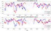 |
Fig. 1. Polarity match percentages between the HMF at 1 AU and the coronal field based on WSO data (rss = 3.5 R⊙, nmax = 9) with T- (blue) and A-sectors (red) defined with the plane division at 1 AU (top panel) or with the radial division in the corona (bottom panel). Rotational values have been smoothed to the running means of 13 rotations. Time of erroneous WSO data is denoted by a dotted line. |
On the other hand, in the bottom panel of Fig. 1 the A-sector has a higher PM percentage than the T-sector in 1985–1986, 2002–2003, 2005, and 2015, while the T-sector has a higher PM than the A-sector in 1977–1978, 1989–1990, 1993–1995, and 2010–2012. Interestingly, most of the times when there is a notable asymmetry in PM percentage between the A- and T-sector are the same in the two panels of Fig. 1, but their asymmetries are opposite. This is particularly true for 1977–1978, 1985–1986, 1993–1995 and 2003–2005, which coincide with the times of the bashful ballerina (Virtanen & Mursula 2014).
To further verify the WSO result, especially because of the error of WSO data in 1996–2001, we have calculated the polarity match percentages also using the synoptic maps from MWO. Figure 2 shows the polarity match percentages between the HMF and the coronal field for the same two sector definitions as in Fig. 1, using the MWO synoptic maps from 1974 to 2012. Figure 2 shows the same pattern of opposite asymmetries between the two polarities for the two sector definitions and verifies the main asymmetries of Fig. 1 in 1985–1986 and 1992–1995. Moreover, MWO data depict no large asymmetry in 1996–2001 contrary to the erroneous WSO data (Fig. 1).
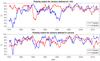 |
Fig. 2. Polarity match percentages between the HMF at 1 AU and the coronal field based on MWO data (rss = 3.5 R⊙, nmax = 9) with T- (blue) and A-sectors (red) defined with the plane division at 1 AU (top panel) or with the radial division in the corona (bottom panel). Rotational values have been smoothed to running means of 13 rotations. |
Figure 3 shows how a southward shift of the HCS/neutral line that is larger in the corona than at 1 AU can explain the different PM percentages in the two cases of sector definition depicted in Figs. 1 and 2. Figure 3 shows, as an example, the case of a negative solar polarity minimum, when the T-sector is dominant in the northern hemisphere, with the simplifying assumption that the whole area above (below) the HCS/neutral line is in the T-sector (A-sector). If we define the sectors at 1 AU, as shown in the top panel of Fig. 3, we get a 100% match for the T-sector, since the whole area of the T-sector observed at 1 AU is mapped to the T-sector in the corona. However, there is a small area (shown in gray shading) within the A-sector at 1 AU which is erroneously mapped to the coronal T-sector, lowering the A-sector match percentage. On the other hand, if we define sectors based on the coronal field, as shown in the bottom panel of Fig. 3, the situation is reversed and the match percentage for A-sector is 100%, and less than that for T-sector. In reality the sector structure distribution is more complicated than the simplified view of Fig. 3, and the actual match percentages are less than 100% even for the sector in the optimum shift configuration.
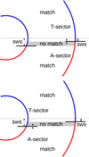 |
Fig. 3. Sketch showing how a larger southward shift (SWS) of the HCS/neutral line (thick horizontal bar) in the corona than in the heliosphere affects the polarity match, depending on whether the T-sector (blue) and A-sector (red) are defined at 1 AU (top panel) or in the corona (bottom panel). |
Accordingly, Fig. 3 predicts that during negative solar polarity times, like in the 1980s and 2000s, when the T-sector (A-sector) is dominant in the northern (southern) hemisphere, the PM for heliospheric T-sector should be larger than for the A-sector and the PM for the coronal T-sector should be smaller than for the corresponding A-sector. During the positive solar polarity times, such as those during the 1970s, 1990s, and 2010s, when the A-sector (T-sector) is dominant in the northern (southern) hemisphere, the reverse is predicted.
Figures 1 and 2 verify these predictions for the declining to minimum phases of solar cycles 21–23 (partly cycle 20). During cycles 20–22 the difference in the PM percentage between the two sectors is large, but during cycle 23 the sectoral asymmetry is weaker and less continuous (Mursula & Virtanen 2011). We also note that if the southward shift of the coronal neutral line was smaller than the HCS shift at 1 AU, the PM percentages would be opposite to those observed. Thus, our results show that the southward shift is indeed larger in the corona than in the heliosphere.
4. Sector asymmetry ratios
Figure 4 shows the annual (T − A)/(T + A) sector asymmetry ratios for 1 AU obtained from OMNI 2 data, and for the solar corona using WSO and MWO synoptic maps. The ratio at 1 AU is calculated by counting the annual number of hours when a T-sector (A-sector) is measured, denoted by T (A). For WSO and MWO the number of T and A hours is calculated based on the sign of the coronal field at the coronal footpoint location of the magnetic field measured at Earth.
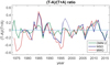 |
Fig. 4. (T − A)/(T + A) ratio measured with OMNI data (green) and predieted using WSO (blue) and MWO (orange) synoptic maps. The erroneous WSO times have been plotted with a dotted line. |
Mursula & Hiltula (2003) first calculated the (T − A)/(T + A) asymmetry ratio for OMNI 2 data, and found a statistically significant variation with the solar 22 year magnetic cycle, implying a southward-shifted HCS. The ratios at 1 AU and in the corona have mostly the same sign in Fig. 4, indicating that the (annually averaged) asymmetry has the same orientation at the two locations. We note, however, that in 1985–1986 (1977–1978, 1992–1995), the T-sector occurrence is considerably larger (smaller) in WSO and MWO data than at 1 AU. Since in 1985–1986 (1977–1978, 1992–1995) the T-sector (A-sector) was dominant in the northern hemisphere, this difference in asymmetry between the corona and 1 AU further verifies the above observations that the neutral line/HCS was shifted more to the south in the corona than at 1 AU. After 2000 the difference in PM percentage between the two locations decreases, in agreement with the smaller differences depicted in Fig. 1.
These results strongly suggest that there was a systematic southward shift in the neutral line/HCS in the 1970s, 1980s, and 1990s, both in the solar corona and in the heliosphere at 1 AU, and that this shift was considerably larger in the corona than at 1 AU. During solar cycle 23 the north-south asymmetry was weaker (Mursula & Virtanen 2011), probably due to the weaker polar fields. Weak polar fields make it easier for random surges of either polarity to destroy the systematic asymmetry of the polar field.
5. Conclusions
We have studied the simultaneous hemispheric asymmetry of coronal and heliospheric magnetic fields with a new, robust method. This involves calculation of the rotational polarity match percentages between the corona and 1 AU separately for the towards and away sectors, and division of the sectors using either the field observed at 1 AU or the coronal field.
Mursula & Hiltula (2003) showed that during solar minima there is a systematic southward shift of the HCS, calling this phenomenon the bashful ballerina. They used hourly OMNI data to calculate the annual ratios of sector occurrence (T − A)/(T + A), and showed that, in the late declining to minimum phase of the solar cycle, the sector dominant in the northern hemisphere is detected more often. Zhao et al. (2005) used the PFSS model with WSO photospheric data to calculate the solid angles occupied by the positive and negative coronal fields, and estimated the north–south HCS displacement from 1976 to 2001. They found a long-lasting interval when the coronal neutral line was southward shifted during the late declining phase of both studied solar cycles 21 and 22. Virtanen & Mursula (2016) extended the Zhao et al. (2005) analysis to show that, according to the six instruments they used, there is a systematic north-south asymmetry in the corona during four solar cycles.
In this paper we present convincing evidence that the southward shift of the neutral line in the corona is larger than the simultaneous HCS shift at 1 AU. This conclusion is based on a systematic difference in the sectoral polarity match (Fig. 1), which depends on whether we define the sectors at 1 AU or in the corona. We have also calculated the annual (T − A)/(T + A) sector occurrence ratios both at 1 AU and in the corona (Fig. 4), and find that during the bashful ballerina years, the ratio at 1 AU is smaller than the ratio in the corona. This further supports the idea of a larger southward shift in the corona than at 1 AU. Our results strongly suggest that the radial evolution of the HMF is different in the northern and southern hemispheres, at least during these specific times that form a considerable fraction of the solar cycle. Although detailed physical explanations will remain the topic of subsequent studies, a possible cause could be related to how the magnetic or plasma pressure evens out the large asymmetry in the heliosphere.
Acknowledgments
We acknowledge the financial support by the Academy of Finland to the ReSoLVE Centre of Excellence (project No. 272157). Wilcox Solar Observatory data used in this study were obtained via the web site http://wso.stanford.edu courtesy of J.T. Hoeksema. Mt. Wilson data was obtained at ftp://howard.astro.ucla.edu/pub/obs/synoptic_charts/ fits /courtesy of Dr. Roger Ulrich. The OMNI data were obtained from the GSFC/SPDF OMNIWeb interface at http://omniweb.gsfc.nasa.gov.
References
- Abramenko, V.,Yurchyshyn, V.,Linker, J.,et al. 2010, ApJ, 712, 813 [NASA ADS] [CrossRef] [Google Scholar]
- Altschuler, M. D., &Newkirk, G. 1969, Sol. Phys., 9, 131 [Google Scholar]
- de Toma, G. 2011, Sol. Phys., 274, 195 [NASA ADS] [CrossRef] [Google Scholar]
- Erdös, G., &Balogh, A. 2010, J. Geophys. Res. Space Phys., 115, A01105 [Google Scholar]
- Hiltula, T., &Mursula, K. 2006, Geophys. Res. Lett., 33, L03105 [NASA ADS] [CrossRef] [Google Scholar]
- Koskela, J. S.,Virtanen, I. I., &Mursula, K. 2017, ApJ, 835, 63 [NASA ADS] [CrossRef] [Google Scholar]
- Linker, J. A.,Caplan, R. M.,Downs, C.,et al. 2017, ApJ, 848, 70 [NASA ADS] [CrossRef] [Google Scholar]
- Lockwood, M.,Rouillard, A. P.,Finch, I., &Stamper, R. 2006, J. Geophys. Res. Space Phys., 111, A09109 [Google Scholar]
- Lukianova, R., &Mursula, K. 2011, J. Atmos. Sol. Terr. Phys., 73, 235 [NASA ADS] [CrossRef] [Google Scholar]
- Mursula, K., &Hiltula, T. 2003, Geophys. Res. Lett., 30, 2135 [Google Scholar]
- Mursula, K., &Virtanen, I. 2011, A&A, 525, L12 [NASA ADS] [CrossRef] [EDP Sciences] [Google Scholar]
- Schatten, K. H.,Wilcox, J. M., &Ness, N. F. 1969, Sol. Phys., 6, 442 [Google Scholar]
- Smith, E. J., &Balogh, A. 1995, Geophys. Res. Lett., 22, 3317 [NASA ADS] [CrossRef] [Google Scholar]
- Ulrich, R. K. 1992, in Cool Stars, Stellar Systems, and the Sun, eds. M. S. Giampapa, & J. A. Bookbinder, ASP Conf. Ser., 26, 265 [Google Scholar]
- Virtanen, I. I., &Mursula, K. 2010, J. Geophys. Res. Space Phys., 115, A09110 [Google Scholar]
- Virtanen, I. I., &Mursula, K. 2014, ApJ, 781, 99 [Google Scholar]
- Virtanen, I., &Mursula, K. 2016, A&A, 591, A78 [NASA ADS] [CrossRef] [EDP Sciences] [Google Scholar]
- Virtanen, I., &Mursula, K. 2017, A&A, 604, A7 [NASA ADS] [CrossRef] [EDP Sciences] [Google Scholar]
- Wang, Y.-M., &Sheeley, N. R., Jr. 1995, ApJ, 447, L143 [NASA ADS] [Google Scholar]
- Wang, Y.-M.,Robbrecht, E., &Sheeley, N. R., Jr. 2009, ApJ, 707, 1372 [NASA ADS] [CrossRef] [Google Scholar]
- Wilcox, J. M., &Ness, N. F. 1965, J. Geophys. Res., 70, 5793 [NASA ADS] [CrossRef] [Google Scholar]
- Zhao, X. P.,Hoeksema, J. T., &Scherrer, P. H. 2005, J. Geophys. Res. Space Phys., 110, A10101 [Google Scholar]
All Figures
|
Fig. 1. Polarity match percentages between the HMF at 1 AU and the coronal field based on WSO data (rss = 3.5 R⊙, nmax = 9) with T- (blue) and A-sectors (red) defined with the plane division at 1 AU (top panel) or with the radial division in the corona (bottom panel). Rotational values have been smoothed to the running means of 13 rotations. Time of erroneous WSO data is denoted by a dotted line. |
| In the text | |
|
Fig. 2. Polarity match percentages between the HMF at 1 AU and the coronal field based on MWO data (rss = 3.5 R⊙, nmax = 9) with T- (blue) and A-sectors (red) defined with the plane division at 1 AU (top panel) or with the radial division in the corona (bottom panel). Rotational values have been smoothed to running means of 13 rotations. |
| In the text | |
|
Fig. 3. Sketch showing how a larger southward shift (SWS) of the HCS/neutral line (thick horizontal bar) in the corona than in the heliosphere affects the polarity match, depending on whether the T-sector (blue) and A-sector (red) are defined at 1 AU (top panel) or in the corona (bottom panel). |
| In the text | |
|
Fig. 4. (T − A)/(T + A) ratio measured with OMNI data (green) and predieted using WSO (blue) and MWO (orange) synoptic maps. The erroneous WSO times have been plotted with a dotted line. |
| In the text | |
Current usage metrics show cumulative count of Article Views (full-text article views including HTML views, PDF and ePub downloads, according to the available data) and Abstracts Views on Vision4Press platform.
Data correspond to usage on the plateform after 2015. The current usage metrics is available 48-96 hours after online publication and is updated daily on week days.
Initial download of the metrics may take a while.