| Issue |
A&A
Volume 617, September 2018
|
|
|---|---|---|
| Article Number | A13 | |
| Number of page(s) | 12 | |
| Section | Astrophysical processes | |
| DOI | https://doi.org/10.1051/0004-6361/201833321 | |
| Published online | 12 September 2018 | |
Multi-zone non-thermal radiative model for stellar bowshocks
1
Instituto Argentino de Radioastronomía (CCT La Plata, CONICET), C.C.5, 1894 Villa Elisa, Buenos Aires, Argentina
e-mail This email address is being protected from spambots. You need JavaScript enabled to view it.
, This email address is being protected from spambots. You need JavaScript enabled to view it.
2
Facultad de Ciencias Astronómicas y Geofísicas, Universidad Nacional de La Plata, Paseo del Bosque, B1900FWA
La Plata, Argentina
3
Departament de Física Quàntica i Astrofísica, Institut de Ciències del Cosmos (ICCUB), Universitat de Barcelona (IEEC-UB), Martí i Franquès 1, 08028
Barcelona, Spain
e-mail This email address is being protected from spambots. You need JavaScript enabled to view it.
4
Institut für Kernphysik (IKP), Karlsruhe Institute of Technology (KIT), Germany
5
Instituto de Tecnologías en Detección y Astropartículas (CNEA, CONICET, UNSAM), Buenos Aires, Argentina
Received:
29
April
2018
Accepted:
21
June
2018
Abstract
Context. Runaway stars produce bowshocks that are usually observed at infrared (IR) wavelengths. Non-thermal radio emission has been detected so far only from the bowshock of BD+43°3654, whereas the detection of non-thermal radiation from these bowshocks at high energies remains elusive.
Aims. We aim at characterising in detail the radio, X-ray, and γ-ray emission from stellar bowshocks accounting for the structure of the region of interaction between the stellar wind and its environment.
Methods. We develop a broadband-radiative, multi-zone model for stellar bowshocks that takes into account the spatial structure of the emitting region and the observational constraints. The model predicts the evolution and the emission of the relativistic particles accelerated and streaming together with the shocked flow.
Results. We present broadband non-thermal spectral energy distributions for different scenarios, synthetic radio-cm synchrotron maps that reproduce the morphology of BD+43°3654, and updated predictions in X-ray and γ-ray energy ranges. We also compare the results of the multi-zone model applied in this work with those of a refined one-zone model.
Conclusions. A multi-zone model provides better constraints than a one-zone model on the relevant parameters, namely the magnetic field intensity and the amount of energy deposited in non-thermal particles. However, one-zone models can be improved by carefully characterising the intensity of the IR dust photon field and the escape rate of the plasma from the shocked region. Finally, comparing observed radio maps with those obtained from a multi-zone model enables constraints to be obtained on the direction of stellar motion with respect to the observer.
Key words: stars: massive / stars: winds, outflows / radiation mechanisms: non-thermal / acceleration of particles
© ESO 2018
1. Introduction
Massive stars have supersonic strong winds that sweep-up and heat the gas and dust from the surrounding interstellar medium (ISM), generating cavities known as wind-blown stellar bubbles. When these stars have a high (supersonic) peculiar velocity with respect to the ISM, the geometry of the bubble becomes bow-shaped instead of spherical (Weaver et al. 1977). The heated ambient dust and gas emit mostly infrared (IR) radiation, which can be detected thus allowing the identification and characterisation of these bowshcks (BSs; Noriega-Crespo et al. 1997, and references therein)
Strong BSs are promising places for the acceleration of relativistic particles, which produce peculiar radiative features throughout the whole electromagnetic spectrum, especially at radio-cm frequencies and at energies above 1 keV (i.e. X-rays and γ-rays; del Valle & Romero 2012). However, despite the large number of such objects observed to date (Peri et al. 2012, 2015; Kobulnicky et al. 2016), BD+43°3654 remains the only one in which non-thermal (NT) radio emission has been observed (Benaglia et al. 2010). Until now, no stellar BS has been detected either at X-rays (Toalá et al. 2016, 2017; De Becker et al. 2017), high-energy γ-rays1 (Schulz et al. 2014), or very high-energy γ-rays (H.E.S.S. Collaboration et al. 2018).
The radio emission at low frequencies is expected to be dominated by synchrotron radiation produced by the interaction of relativistic electrons with the local magnetic field (Ginzburg & Syrovatskii 1964). The detection of NT radio emission is ubiquitous in systems involving shocks, such as collidingwind massive binaries (e.g. Eichler & Usov 1993), supernova remnants (e.g. Torres et al. 2003), and proto-stellar jets (e.g. Marti et al. 1993; Rodríguez-Kamenetzky et al. 2017). This suggests that shocks produced by strong stellar winds (SWs) are suitable for the acceleration of particles (electrons, protons, and heavier nuclei) up to relativistic energies. In this context, diffusive shock acceleration (DSA; Axford et al. 1977; Krymskii 1977; Bell 1978; Blandford & Ostriker 1978) is the most likely mechanism. Furthermore, it is expected that these relativistic particles radiate their energy at energies from radio to γ-rays. A few models have been developed to address the NT emission from stellar BSs (del Valle & Romero 2012, 2014; Pereira et al. 2016), some of which over-predicted the high-energy radiation from these systems.
In this work, we revisit the assumptions of previous emission models for stellar BSs and apply a new multi-zone emission model, presented in Sect. 2, to BSs. In Sect. 3, we present the results of applying this model and discuss them in order to assess future radio, X-ray, and γ-ray surveys that search for NT emission from stellar BSs. We also show synthetic radio-cm synchrotron emission maps that reproduce the available data and radio morphology of BD+43°3654, and make updated predictions for this object in X-rays and γ-rays consistent with the latest observational constraints. The conclusions are summarised in Sect. 4.
2. Model
Most of the NT radiation models presented in the literature rely on the one-zone approximation, which assumes that the emitter can be considered as point-like, that is, homogeneous and of irrelevant size. However, the validity of such models has been questioned in view of the discrepancies between predictions and observations (Toalá et al. 2016). Additionally, the structure of the BS can, in principle, be resolved with current radio interferometers and X-ray satellites, but it is not possible to address correctly issues of the spatial distribution of the emission using one-zone models.
A complete broadband radiative model of the BS needs to take into account the magnetohydrodynamics (MHD) of the stellar wind shock and its evolution, the acceleration of relativistic particles, and the emission of these particles considering inhomogeneous conditions throughout the BS. Here, we develop an extended model for the BS emitter in which we consider analytical prescriptions for the MHD, a DSA mechanism for the acceleration of particles, and a detailed numerical method for the calculation of the particle emission throughout the BS. The details of the model are specified below.
2.1. Geometry
In the reference frame of a moving star, the stellar BS is the result of the interaction of the ISM material acting as a planar wind and the stellar spherical wind. The shape and dynamics of stellar BSs have been studied by several authors (e.g. Dyson 1975; Wilkin 1996; Meyer et al. 2016; Christie et al. 2016). The collision of the SW and the ISM forms an interaction region consisting of a forward shock that propagates through the ISM, a contact discontinuity (CD) between the two media, and a reverse shock (RS) that propagates through the unshocked SW. The CD is the surface where the flux of mass is zero. The reverse shock is adiabatic and fast, whereas the forward shock is radiative and slow (e.g. van Buren 1993). Since DSA works in the presence of strong adiabatic shock waves, we will focus exclusively on the reverse shock. The stagnation point is located at a distance R0 from the star, on the symmetry axis of the BS (with the direction of the stellar motion), and is the point where the ram pressure of the SW and the ISM completely cancel each other out.
For a star with a mass-loss rate Ṁw, wind velocity υw, and a spatial velocity V⋆, moving in a medium of density ρISM, the stagnation point is at (1)
(1)
As R0 ≫ R⋆, it is valid to simply adopt υw = υ∞. Any position on the CD can be determined by an angle θ from the BS symmetry axis, which was characterised by Wilkin (1996) for the case of a cold ISM (i.e. with negligible thermal pressure):  . Christie et al. (2016) generalised this solution for the case of non-negligible thermal pressure in the ambient fluid, opening the possibility to study the BSs in warm or even hot fluids such as accretion disks. According to their results, the width of the shocked stellar wind region at θ is well approximated as H(θ) ≈ 0.2 R(θ).
Following del Palacio et al. (2016), we develop a two-dimensional (2D) model assuming that the BS is an axisymmetric shell of negligible width. Given that the shocked gas flows at a fixed angle ø around the symmetry axis, we can restrict most of our analysis to a one-dimensional (1D) description of a fluid moving in the XY plane. A schematic picture of the model is shown in Fig. 1. The position of a fluid element on the XY plane is solely determined by θ. As the magnetic field is not dynamically relevant, it is considered that a fluid element, upon entering the RS, moves downstream from the BS apex. We assume that NT particles are accelerated once the fluid line enters the RS region, and that these particles flow together with the shocked fluid, which convects the ambient magnetic field2.
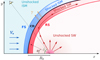 |
Fig. 1. Sketch (not to scale) of the model considered in this work. Despite the axis representation, the (0, 0) position corresponds to the star location. In the star reference frame, the ISM moves with velocity equal to V⋆. The position of the contact discontinuity (CD), forward shock (FS), and reverse shock (RS) are shown in solid lines. The solid line with arrows coming from the star and entering into the shocked region represents one of the streamlines that conform the emitter. The inclination angle i and the position angle θ are also shown. |
The BS radiation is formed by a sum of these 1D emitters (linear emitters hereafter) that are symmetrically distributed around the direction of motion of the star in a three-dimensional (3D) space: each discrete emission cell is first defined in the XY plane, and the full 3D structure of the wind interaction zone is obtained via rotation around the X axis, in the ø direction. The hydrodynamics (HD) and particle distribution have azimuthal symmetry. The dependence with the azimuthal angle arises only for processes that depend also on the line of sight (Sect. 3.3.3).
We assume that the flow along the BS is laminar, neglecting mixing of the fluid streamlines or mixing between shocked wind and medium. The particles are followed up to an angle θ ~ 135°, or equivalently, until they travel a distance ~5 R0. According to our simulations, more than 50% of the emission is produced within θ < 60° (~R0), close to 90% within θ < 120° (≲4 R0), and above 99% within θ < 135°. Therefore, θ ~ 135° is sufficient to capture most of the emission from the injected particles, and it also allows us to capture most of the wind kinetic luminosity available for NT particles.
2.2. Hydrodynamics
The HD of the BS, in particular the shocked SW, depends on the star mass-loss rate, Ṁ, and the wind terminal velocity, υ∞. A stationary approximation is valid as long as V⋆ ≪ υ∞, as the shocked stellar wind leaves the BS before the environment can change significantly. In addition, the SW shock is adiabatic, that is, the shocked stellar wind leaves the BS before radiating its energy, which enhances its stability. Such wind shocks are expected to be quite stable for supersonic (non-relativistic) stars (Dgani et al. 1996).
We apply the analytical HD prescriptions given by Christie et al. (2016) to characterise the values of the relevant thermodynamical quantities in the shocked SW (which we assume to be co-spatial with the CD), and to obtain tangent and perpendicular vectors to the BS surface at each position of the CD. The thermodynamical quantities in the shocked SW rely on the assumption that the fluid behaves like an ideal gas with adiabatic coefficient γad = 5/3, and the application of the Rankine-Hugoniot jump conditions for strong shocks. The magnetic field is obtained by assuming that, at each position, its pressure is a fraction ζB of the thermal pressure: (2)
(2)
The dependence of the thermodynamic quantities with θ is shown in Fig. 2. Near the apex, the incoming SW impacts on the BS surface perpendicularly, leading to a big jump in the gas pressure and temperature, and the fluid practically halts (i.e. quasistagnates). As θ increases, the shock becomes more oblique, the temperature and pressure are lower, and the tangential velocity becomes a substantial fraction of υ∞ (in fact, the fluid can accelerate a bit further because of the pressure gradient).
 |
Fig. 2. Thermodynamic quantities of the shocked SW: temperature (solid), magnetic field (long-dashed), density (short-dashed), pressure (dot-dashed), and tangential velocity (double dot-dashed). Quantities with sub-index zero are evaluated at the apex position (see text). The distance to the apex along the shock is given by |

At large distances from the star, the stellar magnetic field is expected to be toroidal and its intensity to drop with the inverse of the distance to the star (Weber & Davis 1967). An upper limit on the stellar surface magnetic field can therefore be estimated by assuming that the magnetic field in the BS comes solely from the adiabatic compression of the stellar magnetic field lines. Adopting an Alfvén radius rA ~ R⋆, we get B⋆ = 0.25 B(θ) (R(θ)/R⋆) (υ∞/υrot) (Eichler & Usov 1993, and references therein). We note that it is possible that the magnetic fields are strongly amplified or even generated in situ (e.g. Schure et al. 2012, and references therein), and therefore the upper limits we derive for B⋆ could be underestimated.
2.3. Non-thermal particles
The BS produced by the SW consists of hypersonic, non-relativistic, adiabatic shocks, where NT particles of energy E and charge q are likely accelerated via DSA. Assuming diffusion in the Bohm regime, the acceleration timescale can be written as tacc ≈ ηaccE (B c q)−1 s, with ηacc ≫ 1 being the acceleration efficiency (Drury 1983). The energy distribution of the accelerated particles at the injection position is taken as Q(E) ∝ E−p exp (−E/Ecut), where p is the spectral index of the particle energy distribution and Ecut is the cut-off energy, obtained by equating tacc with the minimum between the cooling and escape timescales. The canonical spectral index for DSA in a strong shock is p = 2.
Electrons at each cell of the BS cool through various processes, namely adiabatic losses (work done expanding with the thermal fluid), Bremsstrahlung, synchrotron, and inverse Compton interactions (IC) with the ambient radiation fields, namely IR from dust emission and ultraviolet (UV) photons from the star. An example of the relevant timescales is shown in Fig. 3 for the scenario discussed in Sect. 3.1. Adiabatic losses are not dominant with respect to escape losses in this scenario because of the relatively smooth density evolution (see Fig. 2), although they are the dominant cooling process for electrons with Ee ≲ 1 TeV. For near-equipartition magnetic field values (ζB ~ 1), radiative losses are relevant for electrons with Ee ≳ 100 GeV, as synchrotron dominates their cooling. Otherwise, for modest magnetic field values (ζB ≪ 1) escape losses dominate: convection for electrons with Ee ≲ 1 TeV, and diffusion for Ee ≳ 1 TeV. For protons, on the other hand, the cooling processes taken into account are proton–proton inelastic collisions (p–p) and adiabatic expansion. However, protons do not suffer significant energy losses (Fig. 3) and escape completely dominates: convection for protons with Ep ≲ 1 TeV, and diffusion for Ep ≳ 1 TeV.
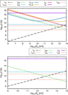 |
Fig. 3. Characteristic cooling and acceleration times for electrons (top panel) and protons (bottom panel) at a position θ = 30° for the generic scenario presented in Table 1. Solid lines are used for cooling processes whereas long dashed lines are used for escape processes. The dotted red line represents the cell convection time (see text in Sect. 2.4). |
When convection dominates the loss time, particles move along the BS with an energy distribution that keeps the same spectral index as the injected distribution. Adiabatic losses slightly soften the particle energy distribution as the particles stream along the emitter. Additionally, for high-energy electrons with Ee ≳ 1 TeV a combination of synchrotron and IC cooling in the Thomson regime can also contribute to a spectral softening. Figure 4 shows the described behaviour for different linear emitters, as well as the total electron distribution and proton distribution at the BS, also calculated for the generic scenario case presented in Sect. 3.1.
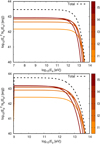 |
Fig. 4. Electron (top panel) and proton (bottom panel) energy distribution for the generic case presented in Table 1. The colour scale represents five different sections (I1–I5) of the emitter that correspond to intervals of length Δθ = 0.15π, starting in θ ɛ [0, 0.15π) for I1, and so on. The black dashed line is the total particle distribution (i.e. the sum of all curves). |
The IC cooling timescale for each photon field was calculated using the formulae given by Khangulyan et al. (2014), suitable for black-body-like spectra. For the case of the stellar UV photon field, we consider that the star emits as a black body with a temperature T⋆ ~ 40 000 K and a dilution factor κ⋆ = [R⋆/(2R(θ))]2, since R(θ) is the distance from the star to the BS at the position θ. The dilution factor is defined by Khangulyan et al. (2014) as the ratio of radiation energy density in the emitter to radiation energy density within a thermal gas. The interaction angle for the scattering process is calculated as the angle between the direction of motion of the emitting electron (which is the line of sight, as the emission is beamed in the direction of the emitting electron) and the radial direction of the stellar photon; naturally, this angle varies with θ. For the case of the IR photon field produced by the dust, we assume isotropy within the NT emitter. Its spectrum is well-approximated with a Planck law of temperature TIR ~ 100 K (Draine 2011; Kobulnicky et al. 2017). The observational evidence shows that the emitting dust usually surrounds the cavity produced by the shocked SW (Kobulnicky et al. 2017). In consequence, if the dust were optically thick, it would be appropriate to set κIR = 1, which was adopted by del Valle & Romero (2012). However, the dust is not strictly optically thick3. This issue has been addressed by De Becker et al. (2017) through the introduction of a “normalization factor” (also known as a grey body). This is equivalent to setting a proper “dilution factor” in the formalism given by Khangulyan et al. (2014). Considering  , the dilution factor of the IR photon field along the BS, κIR(θ) = UIR(θ)/UBB, can be approximated as
 (3)
(3)
where we have considered UIR ≈ LIR/[π R(θ)2c]. As the extended IR radiation is produced in a region of size ~R0 surrounding the NT emitter, the above expression for UIR should be valid, at least, for a region of size ~R0 centred in the apex, and therefore for the brightest portion of the NT emitter. We note that far away from a point-like source (such as the star) the energy density is U = L/(4πr2c), so in the more external regions of the BS we probably overestimate this value. However, if the plasma is not completely optically thin (τ ≲ 1), part of the more internal emission should be reprocessed and isotropised, so we expect that the above expressions serve as a decent approximation even in the outer regions of the NT emitter as well. Moreover, the election of R(θ) in the denominator instead of simply R0 is a phenomenological (not particularly physically motivated) approach to reproduce the observed decay of the IR brightness away from the apex of the BS4. We emphasise that the detailed modelling of the (extended) IR field produces a negligible impact in the NT emission considering that it is produced mostly at distances from the apex ≲R0 (Sect. 2.1). As we show in Sect. 3, the inclusion of a dilution factor for the IR photon field is enough to account for the incompatibility between some of the previous predictions and the upper limits set by recent observations in the X-ray and γ-ray energy bands. We note that even though the energy density of the stellar UV field exceeds the energy density of the dust IR field, cooling due to IC-IR dominates over IC-star for electrons with energies Ee ≳ 200 GeV. This happens because, for the latter, IC takes place much deeper in the Klein-Nishina regime.
The normalisation of the evolved particle distribution depends on the power injected perpendicularly to the shock surface, L w,⊥ ≈ 50% of the total wind power, and on the fraction of that luminosity that goes to NT particles, f NT, which is a free parameter of the model. Given that there is no tight constraint on how the energy is distributed in electrons and protons, we consider two independent parameters fNT,e and fNT,p. It is worth noting that ISM-termination shocks of massive stars may transfer up to a ~10% of their energy into relativistic protons (Aharonian et al. 2018).
2.4. Numerical treatment
We apply the following procedure to obtain the NT particle distribution:
-
We obtain the location of the CD in the XY-plane in discrete points (xi(θi), yi(θi)). We characterise the position of the particles in their trajectories along the BS region through 1D cells (or linear-emitter segments) located at those points.
-
We compute the thermodynamic variables at each position i in the trajectory (Sect. 2.2).
-
The wind fluid elements reach the RS at different locations, from where they are convected along the BS. We simulate the different trajectories by taking different values of imin: the case in which imin = 1 corresponds to a line starting in the apex of the BS, whereas imin = 2 corresponds to a line that starts a bit further in the BS, and so on (Fig. 5). The axisymmetry allows us to compute the trajectories only for the 1D emitters with y ≥ 0.
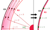
Fig. 5. Illustration of the model for the spatial distribution of NT particles in the BS region. Left panel: different linear emitters, named as j = 1, 2, 3 according to the incoming stellar wind fluid line. Right panel: three cells of a bunch of linear emitters, obtained from summing at each location the contributions from the different linear emitters (see Sect. 2.4).
-
We calculate the power available to accelerate NT particles (either protons or electrons) at each position i as
 (4)
(4)
where
 , and ΔΩ = sin θΔθΔø is the solid angle subtended by the cell. The quantity ΔLNT can be considered as a discrete version of a differential luminosity per surface element.
 -
Relativistic particles are injected in only one cell per linear emitter (that corresponding to imin), and each linear emitter is independent from the rest. For a given linear emitter, particles are injected at a location θi with an energy distribution Q(E, θi) = Q0(θi)E−p exp (−E/Ecut(θi)). The normalisation constant Q0 is set by the condition ∫ E Q(E, θi) dE = ΔLNT(θi), and the particle maximum energy Ecut(θi) by equating the acceleration time to the characteristic loss time, which takes into account both cooling and escape losses. The expressions used to calculate the different timescales are given below.
The particle acceleration timescale is
 (5)
(5)
where the acceleration efficiency is ηacc(θ) = 2πE(c/υ⊥(θ))2. The characteristic escape timescale of the particles is given by
 (6)
(6)
 (7)
(7)
 (8)
(8)
where we consider a characteristic convection timescale, and diffusion in the Bohm regime such that DBohm = rgc/3, where rg = E/(q B) is the gyroradius of the particle.
Denoting nssw the particle number density in the shocked SW, the proton and electron energy losses are
 (9)
(9)
 (10)
(10)
 (11)
(11)
and
 (12)
(12)
 (13)
(13)
 (14)
(14)
 (15)
(15)
respectively.
-
At the injection cell, the steady-state particle distribution is approximated as N0(E, imin) ≈ Q(E) × min (tcell, tcool), where tcell = scell(θ)/υ‖(θ) is the cell convection time (i.e. the time particles spend in each cell).
By the time the relativistic particles reach the next cell in their trajectory, their energy has diminished from E to E′, but the total number of particles must be conserved so that N(E) dE = N(E′) dE′. From that condition we can obtain the evolved version of the injected distribution from
 (16)
(16)
where Ė(E, i) = E/tcool(E, i) is the cooling rate for particles of energy E at the position θi. The energy E′ is given by the condition
 .
. -
We repeat the same procedure varying imin, which represents different linear emitters in the XY-plane.
-
We obtain the total steady-state particle energy distribution at each cell, Ntot(E, i), by summing the distributions N(E, i) obtained for each linear emitter. The result is what we call a bunch of linear emitters, which represents a wedge of width Δø from the total BS structure (calculated at a fixed ø).
-
We can obtain the evolved particle energy distribution for each position (xi, yi, zi ) of the BS surface in a 3D geometry. We achieve this by distributing – via a rotation – the bunch of linear emitters around the axis given by the direction of motion of the star. By doing so, we end up with many bunches of linear emitters, each with a different value of the azimuthal angle ø. The particle energy distribution is the same in all the bunches because of the azimuthal symmetry. We note that the normalisation of the particle energy distribution already takes into account the total number of bunches, as for m ø bunches we take Δø = 2π/m ø in Eq. (4).
2.5. Non-thermal emission
Once the distribution of particles at each cell (xi, yi, zi ) is known, it is possible to calculate the emission at each cell by the previously mentioned radiative processes, and also to obtain the total emission from the modelled region. Radio, X-ray, and γ-ray absorption processes are not relevant given the conditions (size, density, and target fields) of the BS region. The relevant radiative processes are: IC (Khangulyan et al. 2014), synchrotron, p–p, and relativistic Bremsstrahlung (see e.g. Bosch-Ramon & Khangulyan 2009, and references therein). Except for the IC with the stellar UV photons, which depends on the star-emitter-observer geometry, the other radiative processes can be regarded as isotropic, given that the NT particle population is isotropic due to an irregular magnetic field component in the shocked gas. Nevertheless, the presence of an orderly B-component leads to some degree of anisotropy in the synchrotron emission. After calculating the emission at each cell, we can take into account absorption effects along the radiation path if necessary (e.g. free-free absorption of radio photons in the unshocked stellar wind).
2.6. Synthetic radio-emission maps
The total spectral energy distribution (SED) is obtained as the sum of the emission from all the bunches of linear emitters. This SED does not contain all the information available from the model, which can be contrasted with data from spatially resolved radio observations. Therefore, synthetic radio emission maps are valuable complementary information of the morphology predicted by our model, which can help to interpret observations such as the ones reported by Benaglia et al. (2010).
To produce synthetic radio maps at a given frequency, we first project the 3D emitting structure in the plane of the sky, obtaining a 2D distribution of flux (Fig. 6). We then cover this plane adjusting at each location of the map an elliptic Gaussian that simulates the synthesised (clean) beam. If the observational synthesised beam has an angular size a × b, each Gaussian has  and
and  . At each pointing we sum the emission from every location weighted by the distance between its projected position and the Gaussian centre:
  . The result obtained is the corresponding flux per beam at each position.
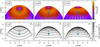 |
Fig. 6. Projected emission maps before (top panel) and after (bottom panel) convolution with a Gaussian beam with σx = σy = 12 arcsec, calculated for the parameters of the generic scenario given in Table 1 but for different inclinations i. The pink cross marks the position of the projected stagnation point, R0 × sin i. The contours in the bottom plots are at 0.05, 0.1, 0.2, 0.4, 0.8, and 1.6 mJy beam−1. |
As shown in Fig. 6, for observing angles i ~ 90° the typical coma-shaped structure of the BS arises (Peri et al. 2012; Kobulnicky et al. 2016). On the other hand, for observing angles i ≲ 45° the BS shape is more circular5 and, additionally, the emission gets very diluted spatially, so it would be difficult to detect such BSs. We also note that the position of R 0,proj lies closer to the star than the position of the maximum of emission; in fact, the maximum emission is always coincident with R0 for values of i > 45° (in angular units). Therefore, when measuring the value of R0 from observational radio emission maps, a factor sin i should not be included.
3. Results
First, we compute the particle energy distribution and the NT emission for a generic scenario using a one-zone model approximation and the extended emission model. We then present analytical estimates of the NT emission dependence with the different system parameters. Finally, we apply our full emission model to the object BD+43°3654.
3.1. One-zone versus multi-zone model
The basics of the one-zone model approximation are addressed by del Valle & Romero (2012). Here we review only two aspects: the characteristic convection timescale and the IR photon field model. Previous one-zone models estimate the convection timescale as tconv ~ H0/υw; however, the shocked fluid takes time to re-accelerate once it impacts on the stagnation point (Fig. 2). Moreover, the emitting area is more extended, similar to R0. We consider that a better estimate of the fluid convection time is tconv ~ R0/cs, where cs is the sound speed in the shocked SW,  . Regarding the modelling of the IR photon field, as discussed in Sect. 2, the assumption of a black-body-emitting surface embedding the emitter is not valid. We consider instead a radiation field approximated as a thermal (black-body-like) spectrum with an energy density of UIR ≈ LIR/(πR02c).
We assume that 10% of the available injection luminosity goes into NT particles, equally distributed between protons and electrons, that is, fNT,e = fNT,p = 0.05. We also fix the magnetic field value adopting an intermediate value ζB = 0.1, which yields B ≈ 20 μG near the apex of the BS; the full list of the selected parameters for this generic scenario is given in Table 1.
Parameters of the generic system we modelled and the system BD+43°3654.
In Fig. 7 we show a comparison of the radiative outputs between the one-zone and the multi-zone models. The one-zone model emission estimates agree with the extended model estimates within a factor of two to three, the largest discrepancies being found in the emission peaks related to the particle maximum energy, and in the IC with the stellar UV photon field. As the anisotropic IC depends on the interaction angle and it varies along the BS structure, we treated the IC-star as isotropic in the one-zone model, as using a single value for i would be completely arbitrary and the impact that it has is quite large. For the extended model, using a value of i = 90° is representative of the produced emission within a factor of two, as shown in Fig. 8.
 |
Fig. 7. Comparison of the SEDs of the generic scenario with the parameters specified in Table 1 using a one-zone model (top panel) and a multi-zone model (bottom panel). The ten-year sensitivity curve of the Fermi satellite is taken from http://fermi.gsfc.nasa.gov, and that of the 100-h CTA from Funk et al. (2013). |
 |
Fig. 8. Comparison of LIC,star for different values of the observing angle i. The simulations are calculated for the generic scenario with the parameters specified in Table 1. |
For both models the available luminosity for NT particles in the BS is Lw,⊥ ≈ 7 × 1035 erg s−1, from which only LNT ≈ 3 × 1034 erg s−1 goes to each particle species. We show the radiated luminosities for both models in Table 2, distinguishing the different contributions. Electrons radiate only ~1% of their power, while for protons the radiated energy fraction is negligible. They escape as cosmic rays to the ISM.
Luminosities produced by the different contributors of each model.
3.2. Analytical estimates on emissivity scaling
As we have shown in Sect. 3.1, the one-zone approximation gives a good estimate of the emission obtained with a more complex model if one takes into account the modifications we propose. Thus, we can rely on the one-zone formalism to make simple estimates on how different system parameters impact on the NT radiative output.
Qualitatively, the NT radio luminosity depends on the ratio tconv/tsy, while the γ-ray luminosity depends on the ratio tconv/tIC. IC-star dominates the SED for photon energies ɛ ≲ 1 GeV, while IC-IR dominates the SED above ≳10 GeV. In the X-ray energy band, synchrotron dominates the NT emission, but a competitive or even dominant thermal contribution is possible6.
Quantitatively, on the one hand,  and
and  . Thus,
  , where we considered
  . As expected, high-velocity stars moving in a dense medium are good candidates, although the most important quantities are intrinsic to the star, and are those related to the stellar wind: the denser and faster this wind is, the better are the chances that its BS will be detectable at radio frequencies. In conclusion, in the search for synchrotron-emitting stellar BSs, it is more important to take into account the individual properties of the star than its runaway conditions. We note that the above scaling is not entirely valid for electrons with E
e > 100 GeV if ζB ~ 1, as in that case synchrotron losses might dominate over convection losses close to the apex, depending on the system parameters.
. As expected, high-velocity stars moving in a dense medium are good candidates, although the most important quantities are intrinsic to the star, and are those related to the stellar wind: the denser and faster this wind is, the better are the chances that its BS will be detectable at radio frequencies. In conclusion, in the search for synchrotron-emitting stellar BSs, it is more important to take into account the individual properties of the star than its runaway conditions. We note that the above scaling is not entirely valid for electrons with E
e > 100 GeV if ζB ~ 1, as in that case synchrotron losses might dominate over convection losses close to the apex, depending on the system parameters.
On the other hand, the γ-ray emission at energies above 10 GeV is dominated by IC with the dust IR photon field as already shown by del Valle & Romero (2012). Assuming that LIR ∝ L⋆nISM and  , which seems coherent and also has some empirical support (Kobulnicky et al. 2017, although with a high dispersion), we have
  . Similar to the synchrotron emission, the most decisive factor determiming LIC,IR is the mass-loss rate of the stellar wind. The above scaling condition is valid if tIC > tconv (Fig. 3). The case for IC cooling dominated by stellar UV photons is similar:
  , so that
  .
.
If we further assume that  (e.g. Fig. 10 from Muijres et al. 2012), then we obtain
  . As the low-frequency radio emission is purely of synchrotron origin, we get
 (17)
(17)
and therefore, the best radio emitting candidates are not necessarily the best γ-ray emitting candidates, as the former prefer faster over denser winds, and the latter have a stronger dependence on the ambient density. In both cases the dependence with υ⋆ coincides.
Finally, we recall that electrons radiate only a small fraction (~ 1%) of their power in the spatial scales considered in the model (Sect. 3.1), whereas protons escape almost with no energy losses. The luminosity injected in both relativistic electrons and protons that escape the modelled BS region is LNT ≈ 3 × 1034 erg s−1. These cosmic rays could cool once they reach a region further downstream, where the BS structure becomes very turbulent or even closes due to the pressure of the ISM (e.g. Christie et al. 2016). However, we do not expect the energy release in the back flow of the BS to be very significant, given the lack of detection of NT emission from stellar BSs. The diffusion and emission from cosmic rays accelerated at stellar BSs of stars moving inside molecular clouds has been studied by del Valle & Romero (2014), although in such environments the target nuclei are more suitable for efficient proton p–p and electron relativistic Bremsstrahlung. Another possibility to take into account is that the laminar approximation of the shocked flow could be relaxed so that mixing between the shocked SW and the shocked ISM could occur. Given that the ambient density in the shocked SW is ~ 0.01 cm−3, whereas nISM ~ 1−10 cm−3, the relativistic Bremmstrahlung and p–p emission could be enhanced by two to three orders of magnitude if mixing is efficient (see e.g. Munar-Adrover et al. 2013, and references therein).
3.3. Application of the model to BD+43°3654
The massive O4If star BD+43°3654, located at a distance of d = 1.32 kpc, has a strong and fast wind that produces a stellar BS. This BS was first identified by Comerón & Pasquali (2007) using infrared data, and it has an extension in the IR sky of 8’. This was the first stellar BS to be detected at radio wavelengths, by Benaglia et al. (2010). In their work, Benaglia et al. (2010) presented Very Large Array (VLA) observations at 1.43 and 4.86 GHz (Fig. 10, top), from which a mean negative spectral index α ≈ −0.5 (with Sν ∝ να) was obtained. Their finding was indicative of NT processes taking place at the BS, in particular relativistic particle acceleration (most likely due to DSA at the shock) and synchrotron emission. This conclusion triggered a series of works on the modelling of the broadband BS emission (del Valle & Romero 2012, 2014; Pereira et al. 2016) using a simplified one-zone approximation. In those works, the radio emission was assumed to be of synchrotron origin, and the radio observations were used as an input to characterise the NT electron energy distribution; the predicted high-energy emission came from IC up-scattering of ambient IR photons by relativistic electrons. Here, we revisit the predictions from the previous radiative one-zone numerical models by applying our more consistent multi-zone model.
The data at radio frequencies allow us to characterise the relativistic electron population, which in turn can be used to model the broadband SED. The NT emission from IR to soft X-rays is completely overcome by the thermal emission from the star and/or the BS, so the SED of NT processes can only be tested in the high-energy (HE) domain, where the NT processes also dominate the spectrum. The electrons that produce the observed synchrotron radiation also interact with the ambient radiation fields, producing HE photons through IC scattering (Benaglia et al. 2010). The relevant HE processes are anisotropic IC with the stellar radiation field and isotropic IC with the dust IR radiation field. The role of secondary pairs in the radiative output is not expected to be relevant (del Valle & Romero 2012).
The reported emission from BD+43°3654 by Benaglia et al. (2010) is consistent with a canonical NT spectral index α = −0.5, which corresponds to an injection index of p = −2α + 1 = 2. However, it is possible that the observed emission is actually the sum of the synchrotron NT emission and a contribution of thermal emission, either from the stellar wind or the BS. The thermal emission has a positive spectral index and, therefore, in order to produce the observed spectrum with α = −0.5, a softer (i.e. more negative) intrinsic NT spectral index would be required. We note, however, that the thermal contribution at low frequencies is likely to be small so a big deviation from p = 2 is not expected. Furthermore, Toalá et al. (2016) derived an upper limit to the X-ray flux in the 0.4–4 keV below 3.6 × 10⁻¹⁴ erg cm−2 s−1 using XMM-Newton observations. That upper limit also seems to favour a softer spectrum (Fig. 9), although the reported value is model-dependent, and it was derived for a power-law photon spectra with index Γ = 1.5; such a spectrum would be appropriate for the synchrotron SED below 0.1 keV, where the slope is ~0.5, but not in the X-ray energy band according to our model7. According to all these remarks, we decided to adopt a softer injection index of p = 2.2, although we note that this value is not tightly constrained.
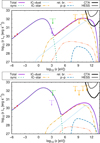 |
Fig. 9. SED for a low (top panel) and a high magnetic field scenario (bottom panel). The red dots represent the VLA flux (Benaglia et al. 2010), the green arrow is the Suzaku upper-limit (UL) in 0.3–10 keV (Terada et al. 2012), the purple arrow the XMM-Newton UL in 0.4–4 keV (Toalá et al. 2016), the orange arrows the Fermi UL in 0.1–300 GeV (Schulz et al. 2014). The grey and black solid lines are the instrument sensitivities for 100-h HESS and 100-h CTA, respectively (Funk et al. 2013). |
Following Brookes (2016), we assume that the star is moving in the warm ISM, with a temperature T
ISM = 8000 K. Christie et al. (2016) addressed the effects of the non-zero ambient thermal pressure in terms of a parameter α
th = P
th/P
kin, which is  for this case. Thus, this introduces only a small correction in the geometry (for instance, R0 ∝ (1 + αth)−1), which we account for only for completeness.
The system spatial velocity is not well determined. The velocity in the plane of the sky is ≈38.4 km s−1 (Brookes 2016, and references therein). Benaglia et al. (2010) used the radial velocity of −66 km s−1 as the radial velocity of the star with respect to the surrounding ISM, which might not be accurate when accounting for Galactic rotation. In fact, if this were the case, the inclination angle should be i ≈ arctan (38.4/66.2) ≈ 30°, whereas the observed emission map favours a high inclination angle i > 60°, which is nearly edge-on. As the radial velocity is for certain negative, we can assume i < 90°. In order to reproduce the observed emission maps, we choose i ≈ 75°, which is consistent with υ⋆ ≈ 40 km s−1. The angular separation to the apex of the BS is R0,proj ≈ 3.2′ (Kobulnicky et al. 2017), although there is some uncertainty when obtaining R 0,proj from the extended emission, as discussed in Sect. 2.6 for the case of radio emission, and for instance Peri (2014) gives a value of R0,proj = 3.5′. In Table 1 we list the adopted system and model parameters.
The wind velocity, υw, is an important parameter in the model as it affects the energy budget of NT particles, the acceleration efficiency, the position of R0, and the convection timescale. In order to maintain a good agreement between our model and the observational constraints, we choose a value of υw ≈ 2300 km s−1, like Peri (2014). We note that Kobulnicky et al. (2018) assume a higher value of υw = 3000 km s−1, but, under the assumption of Bohm diffusion, that leads to a more efficient acceleration, which yields a synchrotron peak at X-rays well above the observational constraints (see Fig. 9). Alternatively, it is possible to reconcile a higher υw if Bohm diffusion is not a good approximation for the acceleration of particles at the BS, turning in practice ηacc into a free parameter in the model (e.g. De Becker et al. 2017).
For the unshocked ISM, we consider a molecular weight μISM = 1.37 (e.g. Kobulnicky et al. 2018), which is only relevant to determine R0. The mean molecular weight in the shocked SW is needed in order to derive the total number of targets for relativistic Bremsstrahlung and p–p interactions; considering that the material is completely ionised, for typical abundances we get μssw = 0.62. With the selected parameters, the equipartition magnetic field at the apex of the BS is ~100 μG, somewhat smaller than the value of ~300 μG estimated by del Valle & Romero (2012). Recall that the magnetic field drops along the BS according to Fig. 2. We are left with only a few free parameters: the value of B in the shocked SW, the fraction fNT,e of energy converted to NT electrons, and the inclination angle. The latter only affects the IC-star SED within a factor of approximately two, as discussed in Sect. 3.1. As we will show in what follows, it is possible to constrain these parameters from the measured radio fluxes and morphological information from the resolved NT radio emission region. With this purpose we explore two extreme scenarios below.
3.3.1. Scenario with low magnetic field
We apply the model described in Sect. 2 to a scenario with a low magnetic field (i.e. ζB ≪ 1). To reproduce the radio observations from Benaglia et al. (2010), we fix the values of the following parameters: i = 75°, fNT,e = 0.16, ζB = 0.01, which leads to B ~ 10 μG and B⋆ < 85 G. We also fix a high value of fNT,p = 0.5 to obtain an upper limit to the p–p luminosity.
The calculated broadband SEDs are shown in Fig. 9, along with some instrument sensitivities and observations from different epochs. The integrated luminosities for each process are Lsy ≈ 8 × 1032 erg s−1, LBr ≈ 2 × 1030 erg s−1, LIC,dust ≈ 5 × 1032 erg s−1, LIC,⋆ ≈ 1033 erg s−1, and Lpp ≈ 4 × 1029 erg s−1. In this case nssw ~ 0.04 cm−3 and nISM ~ 15 cm−3, so relativistic Bremmstrahlung and p–p emission could be enhanced more than three orders of magnitude if mixing is efficient. This would be in tension with the observational upper limits to the γ-ray flux, therefore suggesting that efficient mixing is not likely and that the laminar approximation of the fluid is consistent.
We predict that, in the most favourable case, the system might be detectable at HE by the Fermi satellite. At very HE a detection should wait until the Cherenkov Telescope Array (CTA) becomes operational.
3.3.2. Scenario with equipartition magnetic field
We apply the same model as in Sect. 3.3.1, but with a different value of ζB in order to analyse a scenario with an extremely high magnetic field. We explore the case of ζB = 1, which corresponds to equipartition between the magnetic field and the thermal pressure in the shocked SW (Eq. (2)). Under such conditions the magnetic field would be dynamically relevant (i.e. the magnetic pressure would be a significant fraction of the total pressure in the post-shock region). Nonetheless, we do not alter our prescription of the flow properties, as we adopt a phenomenological model for them only to get a rough approximation of the gas properties in the shocked SW. Besides, our intentions are just to give a semi-qualitative description of this extreme scenario, not to make a precise modelling of the emission, and to obtain a rough estimate of some relevant physical parameters. Fixing ζB = 1 yields B ~ 100 μG in the shocked SW, and, if the magnetic field in the BS is solely due to adiabatic compression of the stellar magnetic field lines, we get B ⋆ < 850 kG on the stellar surface. Such high values of B⋆ are uncommon (Neiner et al. 2015), which suggests that in the energy equipartition scenario the magnetic field in the BS is more likely generated or at least amplified in situ. Setting fNT,e ≈ 0.004 leads to the spectral fit of the fluxes obtained by Benaglia et al. (2010) shown in Fig. 9. There is a tension between the X-ray flux upper limits by Toalá et al. (2016) and the synchrotron emission that extends to energies above 1 keV. This could be either evidence that the magnetic field in BD+43°3654 is not so extreme, or that the particle acceleration efficiency is overestimated. The integrated luminosities for each process for this case are Lsy ≈ 1.7 × 1033 erg s−1, LBr ≈ 4.4 × 1028 erg s−1, LIC,dust ≈ 1.3 × 1031 erg s−1, LIC,⋆ ≈ 2.8 × 1031 erg s−1, and Lpp ≈ 4.3 × 1029 erg s−1.
As the synchrotron cooling time is shorter than the IC cooling time, the bulk of the NT emission is produced in the form of low-energy (<1 keV) photons, and much less luminosity goes into γ-ray production. The value of Lγ obtained is ~102 times smaller than the one obtained in Sect. 3.3.1. This result seems consistent as, roughly, Lsy ∝ fNT,e × ζB, and we are considering a value ~102 times larger for ζB, and therefore fNT,e must be ~102 smaller in order to fit the observations. This thus explains that LIC ∝ fNT,e is a factor ~102 smaller. In this scenario BD+43°3654 is not detectable with the current or forthcoming gamma-ray observatories.
3.3.3. Resolved emission
The full information from the spatially resolved radio observations is only partially contained in the SEDs. Therefore, we compare the morphology predicted by our model with that observed by Benaglia et al. (2010) using VLA observations at two frequencies, 1.42 GHz and 4.86 GHz. We use a synthesised beam of 12 arcsec × 12 arcsec in our synthetic maps so it matches with the synthesized beam of the VLA observations from Benaglia et al. (2010), with a corresponding resolution of 28 arcsec × 28 arcsec (the relation between resolution and beam size is given in Sect. 2.6).
As shown in Sect. 2.6, the morphology of the emission map depends on the inclination angle i. Based on the observed morphology, we can argue that 45° < i < 90°. Figure 10 shows that there is a good agreement between the synthetic map and the observed map for i ~ 75°, both in morphology and emission levels. However, in the modelled map the emission is a bit more extended than the observed one. This could be attributed, for instance, to a magnetic field that drops faster with the apex distance than what our model assumptions predict (Sect. 2.2). A more detailed analysis of the magnetic field structure could be addressed by assuming frozen-in conditions for the magnetic field in each individual line of fluid of the shocked SW. Also, MHD simulations of colliding-wind binaries performed by Falceta-Gonçalves & Abraham (2012) suggest that the magnetic pressure is not a constant fraction of the thermal pressure throughout the shocked plasma. However, the implementation of detailed MHD models for the shocked fluid is beyond the scope of this work.
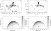 |
Fig. 10. Comparison between the observed radio emission maps taken from (Benaglia et al. 2010; top panel) and our synthetic maps (bottom panel). Top right panel: synthesised beam of 12 arcsec × 12 arcsec is shown (i.e. σx = σy = 12 arcsec). Left and right panels: observing frequency of 1.42 GHz and 4.86 GHz, respectively. The rms levels of the observed maps are 0.3 mJy beam−1 (left panels) and 0.2 mJy beam−1 (right panels). The black solid contours of the 1.42 GHz maps are at 0.9,1.8, 3.0, and 4.5 mJy beam−1, the red dotted contour is at 0.3 mJy beam−1 (the observed map rms), and the green contour is at 6 mJy beam−1 (above the observed values). In the 4.86 GHz maps, the black contours are at 0.6, 1.2, 2.0, and 3.0 mJy beam−1, and the red dotted is at 0.2 mJy beam−1 (the observed map rms). A projection factor cos (Dec) was used for the x-coordinates in the synthetic map in order to relate the synthetic map units to sky positions. |
4. Conclusions
We show that one-zone models can be reconciled with observations by properly accounting for the intensity of the IR dust photon field and motion of the plasma along the shocked region. The multi-zone model we developed improves the constraints on the different model parameters, namely the magnetic field intensity and the amount of energy deposited in NT particles. Our model reproduces fairly well the only radio observations for the object BD+43°3654. However, the free parameters, namely the fraction of available energy that goes into accelerating NT electrons and the magnetic field intensity along the shocked SW, can only be constrained by current facilities (radio interferometers, X-ray and γ-ray satellites) with deep, high-sensitivity observations. Comparison between the synthetic and observed radio maps allows us to constrain the star direction of motion with respect to the observer. Discrepancies in the morphology could account for deviations in the system parameters and/or model hypothesis, such as a highly non-uniform environment or that the magnetic field pressure does not remain a constant fraction of the thermal pressure. Estimating the magnetic field strength in the shocked region allows us to set upper limits for the magnetic field on the stellar surface, thereby inferring whether magnetic field amplification is taking place in the particle acceleration region.
The results presented in this work provide a good insight for future observational campaigns in the radio and γ-ray range. In particular, we show that the most relevant parameters for the radiative output are the mass-loss rate and velocity of the wind of the star, rather than the density of the ISM or the stellar spatial velocity. The NT luminosity (especially the γ-ray luminosity) is strongly dependent on the mass-loss rate, whereas the detailed shape of the SED is defined by the magnetic field strength, the ambient density, and the ratio Ṁ/υw according to Eq. (17). Therefore, deep observations in soft X-rays (0.3−10 keV) could provide tighter constraints to the free parameters in our model, such as the injected particle energy distribution spectral index and the magnetic field strength, through comparison of the synchrotron and IC emission, constraining then the acceleration efficiency. We show that moderate values of the stellar surface magnetic field (B⋆ < 100 G) are sufficient to account for the synchrotron emission even if there is no amplification of the magnetic field besides adiabatic compression; however, if the magnetic field in the BS region is high (≳100 μG), then magnetic field amplification is likely to occur. Low B-values would imply significant gamma-ray emission, whereas high B-values render the predicted gamma-ray radiation undetectable with present or forthcoming instrumentation.
During the review of this article, Sánchez-Ayaso et al. (2018) published a work with a possible association of two Fermi sources with stellar BSs.
We note that the flow is not likely to be completely laminar nor the magnetic field completely ordered, but for simplicity we neglect in this description any macroscopic effect of the turbulent component of the flow and the irregular component of the magnetic field.
The assumption that the dust emits as a black body leads to an overestimation by several orders of magnitude of the observed IR emission, as  .
.
With this prescription the energy density at a position θ in the BS is a factor (R0/R(θ))2 smaller than at the apex.
This is consistent with the statement by Kobulnicky et al. (2016) that BSs with i < 65° are unlikely to be identified as such.
This statement is based in the usage of Eq. (24) from Christie et al. (2016) to estimate the thermal emission from the BS (not shown). However, the simple HD model we use for the BS is not reliable for the calculation of its thermal contribution.
Recall that in the SED ɛ2Nph(ɛ) is plotted, so that the slope is 2 − Γ.
Acknowledgments
We thank the anonymous referee for the detailed and constructive comments. This work is supported by CONICET (PIP2014-0338) and ANPCyT (PICT-2017-2865). SdP acknowledges support by PIP 0102 (CONICET). V.B-R. acknowledges support from MICINN by the MDM-2014-0369 of ICCUB (Unidad de Excelencia “María de Maeztu”). V.B-R. and G.E.R. acknowledge support by the Spanish Ministerio de Economía y Competitividad (MINECO) under grant AYA2016-76012-C3-1-P. The acknowledgment extends to the whole GARRA group.
References
- Aharonian, F., Yang, R., & de Oña Wilhelmi, E. 2018, ArXiv e-prints [arXiv: 1804.02331] [Google Scholar]
- Axford, W. I., Leer, E., & Skadron, G. 1977, International Cosmic Ray Conference, 11, 132 [Google Scholar]
- Bell, A. R. 1978, MNRAS, 182, 147 [NASA ADS] [CrossRef] [Google Scholar]
- Benaglia, P., Romero, G. E., Martí, J., Peri, C. S., & Araudo, A. T. 2010, A&A, 517, L10 [NASA ADS] [CrossRef] [EDP Sciences] [Google Scholar]
- Blandford, R. D., & Ostriker, J. P. 1978, ApJ, 221, L29 [Google Scholar]
- Bosch-Ramon, V., & Khangulyan, D. 2009, Int. J. Mod. Phys. D, 18, 347 [NASA ADS] [CrossRef] [Google Scholar]
- Brookes, D. P. 2016, PhD Thesis, University of Birmingham, UK [Google Scholar]
- Christie, I. M., Petropoulou, M., Mimica, P., & Giannios, D. 2016, MNRAS, 459, 2420 [NASA ADS] [CrossRef] [Google Scholar]
- Comerón, F., & Pasquali, A. 2007, A&A, 467, L23 [NASA ADS] [CrossRef] [EDP Sciences] [Google Scholar]
- De Becker, M., del Valle, M. V., Romero, G. E., Peri, C. S., & Benaglia, P. 2017, MNRAS, 471, 4452 [NASA ADS] [CrossRef] [Google Scholar]
- del Palacio, S., Bosch-Ramon, V., Romero, G. E., & Benaglia, P. 2016, A&A, 591, A139 [NASA ADS] [CrossRef] [EDP Sciences] [Google Scholar]
- del Valle, M. V., & Romero, G. E. 2012, A&A, 543, A56 [Google Scholar]
- del Valle, M. V., & Romero, G. E. 2014, A&A, 563, A96 [NASA ADS] [CrossRef] [EDP Sciences] [Google Scholar]
- Dgani, R., van Buren, D., & Noriega-Crespo, A. 1996, ApJ, 461, 927 [NASA ADS] [CrossRef] [Google Scholar]
- Draine, B. T. 2011, Physics of the Interstellar and Intergalactic Medium (Princeton University Press) [Google Scholar]
- Drury, L. O. 1983, Reports on Progress in Physics, 46, 973 [Google Scholar]
- Dyson, J. E. 1975, Ap&SS, 35, 299 [NASA ADS] [CrossRef] [Google Scholar]
- Eichler, D., & Usov, V. 1993, ApJ, 402, 271 [NASA ADS] [CrossRef] [Google Scholar]
- Falceta-Gonçalves, D., & Abraham, Z. 2012, MNRAS, 423, 1562 [NASA ADS] [CrossRef] [Google Scholar]
- Funk, S., Hinton, J. A., & CTA Consortium. 2013, Astropart. Phys., 43, 348 [NASA ADS] [CrossRef] [Google Scholar]
- Ginzburg, V. L., & Syrovatskii, S. I. 1964, The Origin of Cosmic Rays, authorised english translation edn. (Oxford: Pergamon Press) [Google Scholar]
- H.E.S.S. Collaboration (Abdalla, H., et al.) 2018, A&A, 612, A12 [NASA ADS] [CrossRef] [EDP Sciences] [Google Scholar]
- Khangulyan, D., Aharonian, F. A., & Kelner, S. R. 2014, ApJ, 783, 100 [NASA ADS] [CrossRef] [Google Scholar]
- Kobulnicky, H. A., Chick, W. T., Schurhammer, D. P., et al. 2016, ApJS, 227, 18 [NASA ADS] [CrossRef] [Google Scholar]
- Kobulnicky, H. A., Schurhammer, D. P., Baldwin, D. J., et al. 2017, AJ, 154, 201 [NASA ADS] [CrossRef] [Google Scholar]
- Kobulnicky, H. A., Chick, W. T., & Povich, M. S. 2018, ApJ, 856, 74 [NASA ADS] [CrossRef] [Google Scholar]
- Krymskii, G. F. 1977, Akad. Nauk SSSR Dokl., 234, 1306 [Google Scholar]
- Marti, J., Rodriguez, L. F., & Reipurth, B. 1993, ApJ, 416, 208 [NASA ADS] [CrossRef] [Google Scholar]
- Meyer, D. M.-A., van Marle, A.-J., Kuiper, R., & Kley, W. 2016, MNRAS, 459, 1146 [NASA ADS] [CrossRef] [Google Scholar]
- Muijres, L. E., Vink, J. S., de Koter, A., Müller, P. E., & Langer, N. 2012, A&A, 537, A37 [NASA ADS] [CrossRef] [EDP Sciences] [Google Scholar]
- Munar-Adrover, P., Bosch-Ramon, V., Paredes, J. M., & Iwasawa, K. 2013, A&A, 559, A13 [NASA ADS] [CrossRef] [EDP Sciences] [Google Scholar]
- Neiner, C., Grunhut, J., Leroy, B., De Becker, M., & Rauw, G. 2015, A&A, 575, A66 [NASA ADS] [CrossRef] [EDP Sciences] [Google Scholar]
- Noriega-Crespo, A., van Buren, D., & Dgani, R. 1997, AJ, 113, 780 [NASA ADS] [CrossRef] [Google Scholar]
- Pereira, V., López-Santiago, J., Miceli, M., Bonito, R., & de Castro, E. 2016, A&A, 588, A36 [NASA ADS] [CrossRef] [EDP Sciences] [Google Scholar]
- Peri, C. S. 2014, PhD Thesis, University of La Plata, Argentina [Google Scholar]
- Peri, C. S., Benaglia, P., Brookes, D. P., Stevens, I. R., & Isequilla, N. L. 2012, A&A, 538, A108 [NASA ADS] [CrossRef] [EDP Sciences] [Google Scholar]
- Peri, C. S., Benaglia, P., & Isequilla, N. L. 2015, A&A, 578, A45 [NASA ADS] [CrossRef] [EDP Sciences] [Google Scholar]
- Rodríguez-Kamenetzky, A., Carrasco-González, C., Araudo, A., et al. 2017, ApJ, 851, 16 [NASA ADS] [CrossRef] [Google Scholar]
- Sánchez-Ayaso, E., del Valle, M. V., Martí, J., Romero, G. E., & Luque-Escamilla, P. L. 2018, ApJ, 861, 32 [NASA ADS] [CrossRef] [Google Scholar]
- Schulz, A., Ackermann, M., Buehler, R., Mayer, M., & Klepser, S. 2014, A&A, 565, A95 [NASA ADS] [CrossRef] [EDP Sciences] [Google Scholar]
- Schure, K. M., Bell, A. R., O’C Drury, L., & Bykov, A. M. 2012, Space Sci. Rev., 173, 491 [NASA ADS] [CrossRef] [EDP Sciences] [Google Scholar]
- Terada, Y., Tashiro, M. S., Bamba, A., et al. 2012, PASJ, 64, 138 [NASA ADS] [Google Scholar]
- Toalá, J. A., Oskinova, L. M., González-Galán, A., et al. 2016, ApJ, 821, 79 [NASA ADS] [CrossRef] [Google Scholar]
- Toalá, J. A., Oskinova, L. M., & Ignace, R. 2017, ApJ, 838, L19 [NASA ADS] [CrossRef] [Google Scholar]
- Torres, D. F., Romero, G. E., Dame, T. M., Combi, J. A., & Butt, Y. M. 2003, Phys. Rep., 382, 303 [NASA ADS] [CrossRef] [Google Scholar]
- van Buren, D. 1993, in Massive Stars: Their Lives in the Interstellar Medium eds. J. P. Cassinelli, & E. B. Churchwell, ASP Conf. Ser., 35, 315 [NASA ADS] [Google Scholar]
- Weaver, R., McCray, R., Castor, J., Shapiro, P., & Moore, R. 1977, ApJ, 218, 377 [NASA ADS] [CrossRef] [Google Scholar]
- Weber, E. J. & Davis, Jr., L. 1967, ApJ, 148, 217 [NASA ADS] [CrossRef] [Google Scholar]
- Wilkin, F. P. 1996, ApJ, 459, L31 [NASA ADS] [CrossRef] [Google Scholar]
All Tables
All Figures
|
Fig. 1. Sketch (not to scale) of the model considered in this work. Despite the axis representation, the (0, 0) position corresponds to the star location. In the star reference frame, the ISM moves with velocity equal to V⋆. The position of the contact discontinuity (CD), forward shock (FS), and reverse shock (RS) are shown in solid lines. The solid line with arrows coming from the star and entering into the shocked region represents one of the streamlines that conform the emitter. The inclination angle i and the position angle θ are also shown. |
| In the text | |
|
Fig. 2. Thermodynamic quantities of the shocked SW: temperature (solid), magnetic field (long-dashed), density (short-dashed), pressure (dot-dashed), and tangential velocity (double dot-dashed). Quantities with sub-index zero are evaluated at the apex position (see text). The distance to the apex along the shock is given by |
| In the text | |
|
Fig. 3. Characteristic cooling and acceleration times for electrons (top panel) and protons (bottom panel) at a position θ = 30° for the generic scenario presented in Table 1. Solid lines are used for cooling processes whereas long dashed lines are used for escape processes. The dotted red line represents the cell convection time (see text in Sect. 2.4). |
| In the text | |
|
Fig. 4. Electron (top panel) and proton (bottom panel) energy distribution for the generic case presented in Table 1. The colour scale represents five different sections (I1–I5) of the emitter that correspond to intervals of length Δθ = 0.15π, starting in θ ɛ [0, 0.15π) for I1, and so on. The black dashed line is the total particle distribution (i.e. the sum of all curves). |
| In the text | |
|
Fig. 5. Illustration of the model for the spatial distribution of NT particles in the BS region. Left panel: different linear emitters, named as j = 1, 2, 3 according to the incoming stellar wind fluid line. Right panel: three cells of a bunch of linear emitters, obtained from summing at each location the contributions from the different linear emitters (see Sect. 2.4). |
| In the text | |
|
Fig. 6. Projected emission maps before (top panel) and after (bottom panel) convolution with a Gaussian beam with σx = σy = 12 arcsec, calculated for the parameters of the generic scenario given in Table 1 but for different inclinations i. The pink cross marks the position of the projected stagnation point, R0 × sin i. The contours in the bottom plots are at 0.05, 0.1, 0.2, 0.4, 0.8, and 1.6 mJy beam−1. |
| In the text | |
|
Fig. 7. Comparison of the SEDs of the generic scenario with the parameters specified in Table 1 using a one-zone model (top panel) and a multi-zone model (bottom panel). The ten-year sensitivity curve of the Fermi satellite is taken from http://fermi.gsfc.nasa.gov, and that of the 100-h CTA from Funk et al. (2013). |
| In the text | |
|
Fig. 8. Comparison of LIC,star for different values of the observing angle i. The simulations are calculated for the generic scenario with the parameters specified in Table 1. |
| In the text | |
|
Fig. 9. SED for a low (top panel) and a high magnetic field scenario (bottom panel). The red dots represent the VLA flux (Benaglia et al. 2010), the green arrow is the Suzaku upper-limit (UL) in 0.3–10 keV (Terada et al. 2012), the purple arrow the XMM-Newton UL in 0.4–4 keV (Toalá et al. 2016), the orange arrows the Fermi UL in 0.1–300 GeV (Schulz et al. 2014). The grey and black solid lines are the instrument sensitivities for 100-h HESS and 100-h CTA, respectively (Funk et al. 2013). |
| In the text | |
|
Fig. 10. Comparison between the observed radio emission maps taken from (Benaglia et al. 2010; top panel) and our synthetic maps (bottom panel). Top right panel: synthesised beam of 12 arcsec × 12 arcsec is shown (i.e. σx = σy = 12 arcsec). Left and right panels: observing frequency of 1.42 GHz and 4.86 GHz, respectively. The rms levels of the observed maps are 0.3 mJy beam−1 (left panels) and 0.2 mJy beam−1 (right panels). The black solid contours of the 1.42 GHz maps are at 0.9,1.8, 3.0, and 4.5 mJy beam−1, the red dotted contour is at 0.3 mJy beam−1 (the observed map rms), and the green contour is at 6 mJy beam−1 (above the observed values). In the 4.86 GHz maps, the black contours are at 0.6, 1.2, 2.0, and 3.0 mJy beam−1, and the red dotted is at 0.2 mJy beam−1 (the observed map rms). A projection factor cos (Dec) was used for the x-coordinates in the synthetic map in order to relate the synthetic map units to sky positions. |
| In the text | |
Current usage metrics show cumulative count of Article Views (full-text article views including HTML views, PDF and ePub downloads, according to the available data) and Abstracts Views on Vision4Press platform.
Data correspond to usage on the plateform after 2015. The current usage metrics is available 48-96 hours after online publication and is updated daily on week days.
Initial download of the metrics may take a while.