| Issue |
A&A
Volume 617, September 2018
|
|
|---|---|---|
| Article Number | A8 | |
| Number of page(s) | 14 | |
| Section | Atomic, molecular, and nuclear data | |
| DOI | https://doi.org/10.1051/0004-6361/201833256 | |
| Published online | 12 September 2018 | |
Low-density laboratory spectra near the λ335 channel of the SDO/AIA instrument⋆
1
Physics Division, Physical and Life Sciences, Lawrence Livermore National Laboratory, 94550-9234 Livermore CA, USA
e-mail: This email address is being protected from spambots. You need JavaScript enabled to view it.
2
Astronomisches Institut, Fakultät für Physik und Astronomie, Ruhr-Universität Bochum, 44780 Bochum, Germany
e-mail: This email address is being protected from spambots. You need JavaScript enabled to view it.
Received:
18
April
2018
Accepted:
31
May
2018
Abstract
Aims. For a more complete interpretation of the extreme-ultraviolet (EUV) spectra of the solar corona, it is beneficial to acquire laboratory data of specific chemical elements obtained under coronal conditions.
Methods. The EUV spectra of He, C, N, O, F, Ne, S, Ar, Fe, and Ni in a 30 Å wide wavelength interval near 335 have been excited in an electron beam ion trap.
Results. We observe just under 200 lines, almost half of which are not yet identified and included in spectral models.
Conclusions. Our data serve as a check on atomic databases that are used to interpret solar corona data such as collected by the Solar Dynamics Observatory spacecraft or the EUNIS instrument on sounding rockets. Our findings largely corroborate the databases. However, the accumulated flux of a multitude of mostly weak additional lines is comparable to that of various primary lines.
Key words: Sun: corona / atomic data / methods: laboratory: atomic / techniques: spectroscopic / Sun: UV radiation
Research supported in part by the NASA Heliophysics Technology and Instrument Development for Science Program under award no. NNH16AC82I.
© ESO 2018
1. Introduction
In the past half a century the solar extreme-ultraviolet (EUV) spectrum has been recognized as a rich source of information about the solar environment and is being studied with increasingly sophisticated individual and collaborating devices. Among these, the Solar Dynamics Observatory (SDO) spacecraft with its instruments for high-cadence multiband EUV observations of key spectral features forms a comprehensive tool in the construction of time-resolved temperature maps of the solar corona. The capabilities of the spacecraft and its suite of instruments have been described elsewhere (see Pesnell et al. 2012 and subsequent articles for a comprehensive description of SDO). The high cadence rate of observations is made possible by design and compromise: instead of dispersive EUV spectrometers with their notoriously low efficiencies, the Atmospheric Imaging Assembly (AIA) set of detectors employs multilayer mirrors acting as high-efficiency filters at the cost of a bandwidth on the order of one to 20 Å. The seven EUV bands (λ94, 131, 171, 193, 211, 304, and 335) mainly target various iron lines and He II. Although the individual detectors cannot fully separate the target lines with their particular temperature sensitivities, the combination nevertheless provides a wide-range continuous temperature sensor that works over several decades. At the same time, a grazing incidence grating spectrograph (MEGS-A) of the extreme-ultraviolet variability experiment (EVE) covers a wavelength range that includes all these bands with a spectral resolution of 1 Å and a data cadence of 10 s (Woods et al. 2012).
The SDO/AIA λ335 band comprises Fe XVI and FeXIV lines, which are expected to be bright at relatively high coronal temperatures (as found in flares), as well as lines of Mg, Al, Si, and other elements that are more important at the lower temperatures prevalent in the quiet sun or coronal holes. Any meaningful interpretation of the raw data depends on extensive modeling (O’Dwyer et al. 2010; Parenti et al. 2012). O’Dwyer et al. (2010) list the expected line blends guided by the CHIANTI database (Dere et al. 1997, 2009; Landi et al. 2012; latest updates Landi et al. 2013; Del Zanna et al. 2015) and demonstrate the relative line positions by simulations. The models applied by Parenti et al. (2012) assign a larger role to contributions from lighter elements such as oxygen and neon than is reflected in the simulations by O’Dwyer et al. (2010). Martínez-Sykora et al. (2011) evaluated the roles of dominant and nondominant ion species in the various SDO/AIA detection bands by modeling the (solar) light source and applying more detailed parameters of the filter curves. When combining SDO/AIA and Hinode observations, Del Zanna et al. (2012) have noted that there are problems with unidentified line contaminations. Concerning the band of present interest, Martínez-Sykora et al. (2011) and Boerner et al. (2012) noted that the signal of the SDO/AIA λ335 channel is being contaminated by light of the λ131 channel and by a higher order effect inside the filter system that lets some λ184 light pass. Experience shows that the signals in all AIA bands have to be analyzed in correlation to determine whether the temperature is high or low or in between (and crosstalk has already been noted).
Another example of the interest in this wavelength band is NASA’s Extreme Ultraviolet Normal Incidence Spectrograph (EUNIS; Thomas & Davila 2001), which is a successor to the SERTS instrument, that is being flown on sounding rockets; for a number of measurement campaigns, one of the two observation channels has been 300–370 Å. This instrument has repeatedly been employed for cross-calibrations with spacecrafts such as SOHO and Hinode (Wang et al. 2011). It operates at a resolution close to our instrument (which is described below).
Our laboratory approach complements the interpretation of solar observations. We have shown in the past (see, for example, Beiersdorfer et al. 1999a; Lepson et al. 2002) that laboratory measurements of spectra produced in an electron beam ion trap (EBIT) can be valuable in identifying spectral features by element and often by approximate charge state. Moreover, EBIT spectra repeatedly have shown features that had either been missing from databases or that had not been listed in their natural wavelength positions. Our present measurements of SDO/AIA bands in the laboratory cover the λ335 band and, thus, join our earlier measurements of the lines in the λ131, λ171, λ193, and λ211 bands (Träbert et al. 2014a,b; Beiersdorfer & Träbert 2018; Beiersdorfer et al. 2014a) that have been carried out at high spectral resolution, and a moderate-resolution study of the vicinity of the He II λ304 line (Träbert et al. 2016). The latter study demonstrates the rich spectral content, which in the SDO/AIA λ304 band observations is masked by the strong He line. Our present measurements with their moderate spectral resolution extend our coverage of the λ304 band toward longer wavelengths and provide a practical test of the literature data sets that have been used in the evaluation of the λ335 band data of the SDO/AIA project. We compare our findings with the latest version (v. 8) of the CHIANTI database (Del Zanna et al. 2015) and with the holdings of the NIST online database (Kramida et al. 2015).
The emission we studied is from the elements C, N, O, F, Ne, S, Ar, Fe, and Ni, most of which have a high solar abundance. Measurements on further elements, especially on Mg, Al, Si, and Ca, would also be desirable, but for technical reasons they have to be deferred to another occasion. All of the elements show lines in the neighborhood of the wavelength band of present interest, and many of these lines are not yet listed in the databases used for EUV spectral modeling. Knowing there is a problem related to previously missing lines, modelers can develop bigger spectral models for a given ionization state, compare their models with the data presented, and make progress in identification. We also note that some lines predicted from models do not appear in the prescribed locations, if at all. Thus our work should help to improve the databases and the interpretation of solar data.
2. Measurement
The measurements were performed at the Lawrence Livermore National Laboratory using the EBIT-I electron beam ion trap. The device has been used for laboratory astrophysics measurements for about three decades (Beiersdorfer et al. 2003). In this device, a (quasi-) mono-energetic electron beam of adjustable energy serves to ionize and excite atoms under ultrahigh vacuum conditions. The residual gas pressure is lower than 10−11 mbar. Together with an electron density ne≤1012cm−3, these conditions approximate the dilute plasma conditions of the solar corona.
The materials to be studied are introduced to the trap as a gas of atoms or simple molecules (CO2, N2, SF6, Ne, Ar) or as a molecular vapor of a complex compound (iron as ironpentacarbonyl Fe(CO)5, nickel as nickelocene Ni(C5H5)2). The gas of interest for calibration or data production is injected ballistically at reservoir pressures below 10−7 mbar into the EBIT vessel; the gas plume expands to a pressure well below 10−9 mbar where it traverses the actual trap volume and the energetic and dense electron beam (Träbert et al. 2000). Collisions with the electron beam disintegrate the molecules; any resulting positively charged particles are being trapped in the combination of electric and magnetic fields of a Penning trap plus the space charge effects caused by the electron beam. Trapped ions continue to be exposed to energetic electrons that collisionally excite and ionize the ions up to the limit imposed by the sequence of ionization potentials. The electron beam energy therefore defines the maximum charge state that can be reached in the interplay of ionization and recombination (by electron capture or charge exchange).
The gas flow is continuous, and low charge state ions are replenished all the time. This mode of operation entails that in all spectra there are contributions from low charge state ions; if one wants to produce high charge state ions, the gas injection pressure has to be very low. In order to provide a rough discrimination of charge states, the present measurements were carried out at one to three electron beam energy settings (in the range 300–1000 eV) for most of the injected elements. The highest charge state that in principle can be produced at a given electron beam energy is the lowest one for which the ionization potential exceeds the electron beam energy. In practice, the highest observed charge state is likely lower than the maximum that is achievable in principle because of the aforementioned inflow of neutrals. However, the ionization potentials of most charge states of the light ions (CNOF) are so low that almost all can be highly ionized even at our lowest electron beam energies, which precludes any charge state discrimination of most of our unidentified lines. On the other hand, the spectra of the few-electron ions can be computed well; hence unidentified lines in these cases are more likely to belong to ions with more than three electrons. If the objective is to trace the actual production threshold to learn the ionization potential of the ion that produces a given spectral feature, it is necessary to work at an extremely low injection pressure (resulting in a low signal rate) and to increase incrementally the electron beam energy in much smaller steps than was done here (see the examples set by Lepson et al. 2000, 2002, 2005).
For wavelengths up to 230 Å we used (see Träbert et al. 2014a,b; Beiersdorfer et al. 2014a) our high-resolution grazing-incidence grating spectrographs (HIGGS; Beiersdorfer et al. 2004, 2014b) with a resolving power in the same class as the grating instruments on board Chandra (den Herder et al. 2001) and Hinode (Culhane et al. 2007). The SDO/AIA 335 band of interest here lies beyond the working range of this high-resolution instrument. Instead, we used a medium-resolution flat-field spectrograph, dubbed the long wavelength extreme ultraviolet spectrometer (LoWEUS; Beiersdorfer et al. 1999b), which was equipped with a 1200 ℓ/mm R = 5 m grating, operating at an angle of incidence of 87°. This instrument is the same as was used for the SDO/AIA λ304 band (Träbert et al. 2016) and is similar to those employed on the National Spherical Torus Experiment (NSTX) and the Alcator C-Mod tokamak (Lepson et al. 2012; Graf et al. 2008; Reinke et al. 2010). As was the case in our other measurements, we used a cryogenically cooled CCD camera of 1340 × 1300 pixels of 20 μm × 20 μm each to record the spectra.
Spectra were accumulated for 30–60 min each, filtered for cosmic ray events, and intercompared for irreproducible signal that might have passed the filtering process. The slightly quadratic wavelength calibration curve was adjusted by reference to known spectral lines mostly of light elements (He, N, O), as well as those of Fe (see Kelly 1987; Kramida et al. 2015). The spectrograph setting was chosen to cover the wavelength range from 200 Å to about 450 Å, which includes the SDO/AIA bands 211 Å, 304 Å, and 335 Å in first order of diffraction. We concentrate on those lines that fall into the 320–350 Å region containing the 335 Å channel of the AIA in first diffraction order.
The line width of the grating spectrograph is almost independent of wavelength. Hence first and second diffraction order lines cannot be discriminated by line width. Incidentally, the second diffraction order of one of the strongest solar EUV lines of Fe, the Fe IX line at λ171.07, falls inside the SDO/AIA λ335 band. Owing to observations of the λ171 band (using one of the aforementioned high-resolution spectrographs) we have spectra (Beiersdorfer & Träbert 2018) that we can use to judge the line position and intensity pattern expected of second-order lines contaminating the first-order spectra in the λ335 band. We consider as unknown only lines that are not known in their first-order position in the λ335 band and that do not coincide with second-order images of lines we have observed in the λ171 band (whether identified there or not).
Our detector sees lines about 300 mÅ wide (FWHM) and hence our spectrograph reaches a resolving power R = λ/Δλ≈ 1100 in first order of diffraction. This is a factor of three higher than the MEGS-A grazing incidence grating spectrograph of the EVE experiment on board SDO achieves (Woods et al. 2012), and about 1/80 of the 25-Å half width of the SDO/AIA λ335 channel band pass.
3. Data and analysis
In the present context we consider only lines listed in CHIANTI version 8 (Del Zanna et al. 2015) or the NIST online database (Kramida et al. 2015) as “known”. The NIST data tables have directly observed wavelengths, wavelengths deduced (via the Ritz principle) from energy levels (however determined), and computed table entries. Unfortunately, neither set of wavelength data is complete. We quote the individual NIST table wavelengths, whether directly measured or derived, by subjective assumption. This ambiguity is lower than the wavelength uncertainty interval of our present observations, but it underlines the need for continued spectroscopic investigation. The CHIANTI list is the prime reference for the spectrum simulations performed by O’Dwyer et al. (2010). In a recent evaluation of iron lines (Beiersdorfer & Lepson 2012) CHIANTI was found to be more reliable than the NIST database. Many lines we observe remain unidentified for now (except for the element). However, the wavelength accuracy is sufficient to identify the known lines without problems; it is thus just as sufficient to provide guidance to the eventual identification of the unknown lines. Certainly our measured wavelengths are more accurate than most calculations.
Relative line intensities are important for line identification purposes. However, the production of a given charge state depends on the electron beam energy and thus may differ drastically from one spectrum to the other, if an ionization threshold is being crossed within a series of spectral recordings, or very little, if the beam energy exceeds the threshold to begin with. Hence meaningful relative line intensities can be derived from our spectra only for lines that are known to belong to a given ion species and charge state. Because of the only moderate spectral resolution, a large number of insufficiently resolved weak lines may appear as a continuum underlying the spectrum. Indeed, in some of our other measurements in the SDO/AIA bands the resolving power is much higher, but not all lines can be resolved either. The known problem of true and pseudo continua is further compounded by the fact that the read-out noise of a CCD detector may appear structured. Hence the relative intensities of weak lines are even more uncertain than the straightforward statistical uncertainty of a fit result may suggest. We indicate gross relative line intensities, assigning a value of ten to the strongest line within an individual spectrum. Such a relative intensity information within a given charge state from EBIT measurements is sufficient to match the accuracy of theoretical modeling data and thus to help line identification, even if the theoretical data are shifted in wavelength. We note that EBIT operates with a quasi-monoenergetic electron beam that implies an upper limit to the charge states reached; this technical limit is the basis for our estimate of charge state of unidentified lines. The near-Maxwellian electron energy distribution in the solar corona, however, can produce some high charge state ions even at low temperature.
Carbon and oxygen. The two major lists of reference data, NIST and CHIANTI, have very few carbon lines that are expected to show up in our spectra. It is, of course, possible that among the unidentified lines that we observe when injecting CO2 (Fig. A.1) there are lines that actually belong to C ions, even as almost all identified lines originate from oxygen (Table A.1). The lower part of the same figure shows observations of the SDO/AIA λ171 band range that have been made using our high-resolution spectrograph HIGGS (Beiersdorfer et al. 2004, 2014b) in the course of recording data for our SDO/AIA λ band study (Beiersdorfer & Träbert 2018). The first-diffraction order wavelength scale of these data plots has been adjusted to match the apparent wavelength scale at which the λ171 band data would appear in second diffraction order, but without a correction for the even higher resolving power under such conditions. The narrow line profiles are advantageous for spectral analysis and for indicating the positions of the second order images. We assume that over the narrow wavelength band of either observation, the detection efficiency is practically constant. A convolution with a wider line profile would be necessary to mimic the line widths of our less highly resolved direct observations of the λ335 band. However, even without such a manipulation it is straightforward to identify (approximately) the contribution of second diffraction order light to the envelope of the 355 observations. Near λ171 and λ172 there are strong lines of oxygen (O v and O VI). The strong second order images of these does not affect the SDO/AIA observations that use a multilayer mirror as a wavelength band selector instead of a grating instrument. However, the many unidentified first-diffraction order C or O lines might be worth including in a model of the solar signal once their charge states can be established.
Nitrogen. Spectra of nitrogen were obtained at an electron beam energy of 1000 eV (Fig. A.2). The N iv 2p–3d singlet transition has a wavelength near λ335 and thus is close to the position of the Fe xvi line of primary interest in this SDO/AIA band. This line may be worth including in the solar data analysis, considering that nitrogen has a solar abundance that is about three times higher than iron. The second-diffraction order lines (marked by “2”) of nitrogen and oxygen in our spectra do not affect the SDO data. Known nitrogen lines and unidentified lines are given in Table A.2.
Fluorine and sulfur. Fluorine and sulfur are easily introduced into EBIT as SF6 gas, which, however, implies that it is not immediately known whether an observed spectral line belongs to F or S. Fluorine is not very abundant in the sun and no fluorine lines are listed by CHIANTI. The NIST tables list only two F vii lines in the λ320-350 band, near λ335 (see Table A.3), which we see but weakly in our spectra (Fig. A.3). One strong line in our spectra, near λ332, coincides with the unresolved second diffraction order image of a pair of F v lines (near λ166) that should not affect the SDO/AIA λ335 channel.
Our spectra, recorded at electron beam energies of 300, 600, and 1000 eV, show a large number of unidentified lines that we assume to belong to sulfur, and of which the line at 338.7 Å might affect the SDO/AIA observations. The spectra also show a line pair near λ345 that resembles the strong O v and O vi lines near λ172 and λ173, respectively (in second diffraction order), but at different relative line intensities and with a slightly different spacing. Thus in our spectra a blend of sulfur (several weak lines in first diffraction order) or fluorine with oxygen lines (in second diffraction order) is likely. We note that the CHIANTI database has fewer wavelength listings than the NIST tables in this wavelength range, although we would naively expect 2s–2p transitions (between relatively low-lying levels) to be noticeable. However, most of these transitions are between displaced terms, and these are hardly populated in a low-density environment. This may also explain some relatively large wave-length changes between CHIANTI versions 7.1 and 8 for some entries.
Neon. Neon spectra were recorded at electron beam energies of 300, 600, and 1000 eV. A sample spectrum recorded at 1000 eV is shown in Fig. A.4. Known and other observed lines are given in Table A.4. Only about a dozen of the weaker lines we see are listed in the NIST and CHIANTI tables as belonging to Ne iii in first diffraction order. However, many other lines coincide with the second diffraction order positions of Ne ii through Ne v lines, which should not affect the AIA observations. This leaves about 14, individually relatively weak, neon lines inside the SDO/AIA band λ335.
Argon. Neither the NIST database nor CHIANTI has prominent Ar lines in the λ320–350 wavelength band. Actually, among the two databases, six Ar v lines are considered as known in this wavelength interval. Owing to our use of a reflection grating spectrograph, we also expect second diffraction order images of various Ar VIII to Ar XIII lines. Our Ar spectra were recorded at electron beam energies of 300, 600, and 1000 eV; for an example recorded at 1000 eV, see Fig. A.5. The spectra show about two dozen lines that clearly vary with the electron beam energy. Many of the lines, however, appear in second diffraction order. Among these are lines of O V and O VI. The Ar lines we observe are given in Table A.5. We note that the CHIANTI wavelengths of the Ar X 2s22p5–2s2p6 line doublet differ substantially (by about 0.8 Å) from the NIST listings. There are lines of corresponding brightness in our spectra (in two diffraction orders) only at the positions (λ165.538, 170.642) given by the NIST listing, indicating that in this case the NIST database has better wavelengths than CHIANTI. Another puzzle is the line at 335.2 Å, which fits in wavelength to the second diffraction order of an Ar xii line listed by both CHIANTI and NIST, but which we do not see in the corresponding first diffraction order spectrum. At λ327.8, the observed line is much more intense than the lines that nearby, at 328 Å, might show in second diffraction order. In the SDO/AIA λ335 band overall, there are numerous unidentified Ar lines, but these do not contribute much flux.
Iron. Iron as the dominant contributor to the signal of the λ335 SDO/AIA band was studied at six electron beam energies from 300 to 2600 eV. An example of our λ320–350 spectra (recorded at 1000 eV) is shown in Fig. A.6. O’Dwyer et al. (2010) named the Fe xvi line at λ335.41 as the dominant feature in the λ335 SDO/AIA band, which is blended in our measurement with Fe IX and Fe XII lines to form the third brightest line in this range, and a much weaker Fe XIV line nearby at λ334.18. O’Dwyer et al. (2010) expected the Fe xvi line to be about 20 times stronger than the Fe xiv line in a solar active region. Fits to our data show a ratio on the order of 12 (see Table A.6), which is in the same ball park as the model. Part of the λ335.3 line intensity arises from blending contributions. With several components of the blend separated by much less than a line width, the relative intensities of the components as returned by a line profile fit (unconstrained by a spectral model) are ambiguous. The fourth and fifth most intense lines are second diffraction order lines of Fe IX and Fe X (near λ171), which are well known.
We note that in addition to the aforementioned Fe XIV line at λ335.41 there is a group of lines presumably from lower charge states that in our spectra (with continuous gas injection) are as high in amplitude as the Fe XIV line, and these unidentified lines together provide even more signal flux than that individual known line. The wavelengths of the observed lines, many of the weak lines being hardly resolved, are given in Table A.6.
From the table it becomes evident that the low charge states up to Fe viii have a number of lines in the wavelength range of interest, but we cannot resolve many of those. Moreover, in the range 330–340 Å a number of Fe VII and Fe VIII lines (see Beiersdorfer & Träbert 2018; Del Zanna 2009a,b) have their second-diffraction order images. These lines are numerous, but in our λ171 band first-diffraction order observations they are individually weak. In second diffraction order these lines are expected to remain weak (at most). We do not list these lines, although they contribute to the present spectra, because they are not expected to affect the AIA data for the λ335 channel. For the sake of completeness we included in Table A.6 highly charged Fe ions beyond Fe XVII.
Table A.6 shows how the NIST and CHIANTI reference tables agree or disagree with each other, from agreement of the stated wavelengths through disagreements by some 30 mÅ or even 160 mÅ (Fe xvii near λ323.5) to coverage in only one of the tables and not the other (especially pronounced for iron in the wavelength range of present interest). With our present measurements, however, we cannot resolve the wavelength discrepancies between the two databases.
Nickel. Nickel spectra have been observed at electron beam energies of 300, 600, 1000, and 1600 eV. Similar to the case of Fe, we see little of the known low or very high charge state lines. A sample spectrum (recorded at 1000 eV) with many bright features is shown in Fig. A.7. The prominent lines in our spectrum of the λ335 channel range are second diffraction order images of lines that in first diffraction order would fall into the SDO/AIA λ171 band and which should not affect the AIA λ335 channel signal. This observation supports the recognition by O’Dwyer et al. (2010) that Ni is not an important ingredient of their model for the λ335 band. The wavelengths of our observed lines are given in Table A.7. This table lists wavelengths from the NIST and CHIANTI databases; while there is agreement among the two in many cases, there is also disagreement by up to 100 mÅ in other cases, plus cases in which only one or the other database holds entries.
4. Discussion
The present measurements at an EBIT demonstrate how many unidentified lines of a few given elements appear in survey spectra recorded under conditions that resemble many astrophysical plasmas. The present spectra illustrate the need for additional work, ideally with higher resolution and finer electron beam energy steps, to identify the many unknown new features.
Overall, we observe about 185 spectral lines in the vicinity of the SDO/AIA λ335 band. Almost half of the lines cannot be identified from the NIST and CHIANTI databases, the latter of which is a primary resource for the interpretation of the SDO data. While most of the new lines are weak, when taken together they represent a flux that is on the same order as that of various stronger lines that are used in the spectral model, and thus an, at least approximate, inclusion of the many new lines might benefit the SDO data interpretation.
Acknowledgments
This work was performed under the auspices of the US Department of Energy by Lawrence Livermore National Laboratory under Contract DE-AC52-07NA27344. E.T. acknowledges support from the German Research Association (DFG; grants Tr171/18 and Tr171/19).
References
- Beiersdorfer, P., & Lepson, J. K. 2012, ApJS, 201, 28 [NASA ADS] [CrossRef] [Google Scholar]
- Beiersdorfer, P., & Träbert, E. 2018, ApJ, 854, 114 [NASA ADS] [CrossRef] [Google Scholar]
- Beiersdorfer, P., Lepson, J. K., Brown, G. V., et al. 1999a, ApJ, 519, L185 [NASA ADS] [CrossRef] [Google Scholar]
- Beiersdorfer, P., Crespo López-Urrutia, J. R., Springer, P., Utter, S. B., & Wong, K. L. 1999b, Rev. Sci. Instr., 70, 276 [NASA ADS] [CrossRef] [Google Scholar]
- Beiersdorfer, P., Behar, E., Boyce, K. R., et al. 2003, Nucl. Inst. Meth. Phys. Res. B, 205, 173 [NASA ADS] [CrossRef] [Google Scholar]
- Beiersdorfer, P., Magee, E. W., Träbert, E., et al. 2004, Rev. Sci. Instr., 75, 3723 [NASA ADS] [CrossRef] [Google Scholar]
- Beiersdorfer, P., Träbert, E., Lepson, J. K., Brickhouse, N. S., & Golub, L. 2014a, ApJ, 788, 25 [NASA ADS] [CrossRef] [Google Scholar]
- Beiersdorfer, P., Magee, E. W., Brown, G. V., et al. 2014b, Rev. Sci. Instr., 85, 11E422 [CrossRef] [Google Scholar]
- Boerner, P., Edwards, C., Lemen, J., et al. 2012, Sol. Phys., 275, 41 [NASA ADS] [CrossRef] [Google Scholar]
- Brinkman, A. C., Gunsing, T., Kaastra, J., et al. 2000, Proc. SPIE, 4012, 81 [NASA ADS] [CrossRef] [Google Scholar]
- Brosius, J. W., Rabin, D. M., Thomas, R. J., & Landi, E. 2008, ApJ, 677, 781 [NASA ADS] [CrossRef] [Google Scholar]
- Culhane, J. L., Harra, L. K., James, A. M., et al. 2007, Sol. Phys., 243, 19 [Google Scholar]
- Del Zanna, G. 2009a, A&A, 508, 501 [NASA ADS] [CrossRef] [EDP Sciences] [Google Scholar]
- Del Zanna, G. 2009b, A&A, 508, 513 [NASA ADS] [CrossRef] [EDP Sciences] [Google Scholar]
- Del Zanna, G. O’Dwyer, B., & Mason, H. E. 2011, A&A, 535, A46 [NASA ADS] [CrossRef] [EDP Sciences] [Google Scholar]
- Del Zanna, G., Dere, K. P., Young, P. R., Landi, E., & Mason, H. E. 2015, A&A, 582, A56 [NASA ADS] [CrossRef] [EDP Sciences] [Google Scholar]
- den Herder, J. W., Brinkman, A. C., Kahn, S. M., et al. 2001, A&A, 365, L7 [NASA ADS] [CrossRef] [EDP Sciences] [Google Scholar]
- Dere, K. P., Landi, E., Mason, H. E., Monsignori Fossi, B. C., & Young, P. R. 1997, A&AS, 125, 149 [NASA ADS] [CrossRef] [EDP Sciences] [Google Scholar]
- Dere, K. P., Landi, E., & Young, P. R. 2009, A&A, 498, 915 [NASA ADS] [CrossRef] [EDP Sciences] [Google Scholar]
- Graf, A. T., Brockington, S., Horton, R., et al. 2008, Can. J. Phys., 86, 307 [NASA ADS] [CrossRef] [Google Scholar]
- Kelly, R. L. 1987, J. Phys. Chem. Ref. Data, 16 [Google Scholar]
- Kramida, A., Ralchenko, Yu., Reader, J., & NIST ASD Team 2015, NIST Atomic Spectra Database (ver. 5.3) (Gaithersburg, MD: National Institute of Standards and Technology). Available: http://physics.nist.gov/asd [Google Scholar]
- Landi, E., Del Zanna, G., Young, P. R., Dere, K. P., & Mason, H. E. 2012, ApJS, 744, 99 [NASA ADS] [CrossRef] [Google Scholar]
- Landi, E., Young, P. R., Dere, K. P., Del Zanna, G., & Mason, H. E., 2013, ApJS, 763, 86 [NASA ADS] [CrossRef] [Google Scholar]
- Lemen, J. R., Title, A. M., Akin, D. J., et al. 2012, Sol. Phys., 275, 17 [NASA ADS] [CrossRef] [Google Scholar]
- Lepson, J. K., Beiersdorfer, P., Brown, G. V., et al. 2000, Rev. Mex. Astron. Astrofis., 9, 137 [Google Scholar]
- Lepson, J. K., Beiersdorfer, P., Brown, G. V., et al. 2002, ApJ, 578, 648 [NASA ADS] [CrossRef] [Google Scholar]
- Lepson, J. K., Beiersdorfer, P., Behar, E., & Kahn, S. M. 2005, Nucl. Inst. Meth. Phys. Res. B, 235, 131 [NASA ADS] [CrossRef] [Google Scholar]
- Lepson, J. K., Beiersdorfer, P., Clementson, J., et al. 2012, Rev. Sci. Instr., 83, 10D520 [CrossRef] [Google Scholar]
- Martínez-Sykora, J., De Pontieu, B., Testa, P., & Hansteen, V. 2011, ApJ, 743, 23 [NASA ADS] [CrossRef] [Google Scholar]
- Mewe, R., Kaastra, J. S., & Liedahl, D. A. 1995, Legacy, 6, 16 [Google Scholar]
- O’Dwyer, B., Del Zanna, G., Mason, H. E., Weber, M. A., & Tripathi, D. 2010, A&A, 521, A21 [NASA ADS] [CrossRef] [EDP Sciences] [Google Scholar]
- Parenti, S., Schmieder, B., Heinzel, P., & Golub, L. 2012, ApJ, 754, 66 [Google Scholar]
- Pesnell, W. D., Chamberlin, P. C., & Thompson, B. J. 2012, Sol. Phys., 275, 3 [NASA ADS] [CrossRef] [Google Scholar]
- Reinke, M. L., Beiersdorfer, P., Howard, N. T., et al. 2010, Rev. Sci. Instr., 81, 10D736 [CrossRef] [PubMed] [Google Scholar]
- Thomas, R. J., & Davila, J. M. 2001, Proc. SPIE, 4498, 161 [NASA ADS] [CrossRef] [Google Scholar]
- Träbert, E., Beiersdorfer, P., Utter, S. B., et al. 2000, ApJ, 541, 506 [NASA ADS] [CrossRef] [Google Scholar]
- Träbert, E., Beiersdorfer, P., Brickhouse, N. S., & Golub, L. 2014a, ApJS, 211, 14 [NASA ADS] [CrossRef] [Google Scholar]
- Träbert, E., Beiersdorfer, P., Brickhouse, N. S., & Golub, L. 2014b, ApJS, 215, 6 [NASA ADS] [CrossRef] [Google Scholar]
- Träbert, E., Beiersdorfer, P., Brickhouse, N. S., & Golub, L. 2016, A&A, 586, A115 [NASA ADS] [CrossRef] [EDP Sciences] [Google Scholar]
- Wang, T., Thomas, R. J., Brosius, J. W., et al. 2011, ApJS, 197, 32 [NASA ADS] [CrossRef] [Google Scholar]
- Woods, T. N., Eparvier, F. G., Hock, R., et al. 2012, Sol. Phys., 275, 115 [Google Scholar]
Appendix A: Tables and figures
 |
Fig. A.1. Spectrum of carbon and oxygen in the range λ320–λ350: the spectrum in the middle panel was recorded using our moderate-resolution LoWEUS spectrograph at the EBIT-I electron beam ion trap at an electron beam energy of 700 eV. Identified spectral features are labeled by the corresponding spectrum. Several oxygen lines appear in second diffraction order (marked “2”). The lowest panel of the figure shows a high-resolution spectrum (from our HIGGS spectrograph) at half the wavelength. Strong first-diffraction order lines in this spectrum may appear in second diffraction order in the spectrum in the middle panel. The approximate band pass function of the SDO/AIA λ335 channel is indicated in the top panel. |
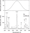 |
Fig. A.2. Spectrum of nitrogen in the range λ320–λ350: the spectrum was recorded with our moderate-resolution LoWEUS spectrograph at the EBIT-I electron beam ion trap at an electron beam energy of 1000 eV. The line markers from fits to the data are visual aids only as the actual number of line components that in spectral line fits of blends can be discerned may depend on the available spectral resolution. Identified spectral features are labeled by the corresponding spectrum. Lines that are recognized as second diffraction order images are denoted “2”. The approximate band pass function of the SDO/AIA λ335 channel is indicated in the top panel. The second-diffraction order oxygen lines indicated are the same as in Fig. A.1, where a high-resolution measurement of these lines in first diffraction order is also shown. |
Lines observed in EBIT within the wavelength band 320–350 when injecting CO2.
Nitrogen lines observed in EBIT-I within the wavelength band λ320–λ350.
Fluorine or sulfur lines observed in EBIT-I within the wavelength band λ320–λ350.
 |
Fig. A.3. Spectrum of fluorine and sulfur in the range λ320–λ350: the spectrum in the middle panel was recorded with our moderate-resolution LoWEUS spectrograph at the EBIT-I electron beam ion trap at an electron beam energy of 1000 eV. Visually recognized line positions are denoted. The lowest panel of the figure shows a high-resolution spectrum at half the wavelength, obtained using our HIGGS instrument. Strong first-diffraction order lines in this spectrum may appear in second diffraction order in the spectrum in the middle panel. Identified spectral features are labeled by the corresponding spectrum. We note the presence of several (known) O and F lines with wavelengths of 160 to 173 Å, the second diffraction order images (denoted “2”) of which appear in the range of the SDO/AIA λ335 band, but would not affect the observations with SDO/AIA. The approximate band pass function of the SDO/AIA λ335 channel is indicated in the top panel. |
 |
Fig. A.4. Spectrum of neon in the range λ320–λ350: the spectrum in the middle panel was recorded with our moderate-resolution LoWEUS spectrograph at the EBIT-I electron beam ion trap at an electron beam energy of 1000 eV. The approximate band pass function of the SDO/AIA λ335 channel is indicated in the top panel. Of the 59 lines seen in this spectrum (with eye-guiding markers), known second diffraction order images are denoted “2”. The lowest panel of the figure shows a high-resolution spectrum at half the wavelength. Strong first-diffraction order lines in this spectrum may appear in second diffraction order in the spectrum in the middle panel. |
Neon lines observed in EBIT-I within the wavelength band λ320–λ350.
 |
Fig. A.5. Spectrum of argon in the range λ320–λ350: the spectrum in the middle panel was recorded with our moderate-resolution LoWEUS spectrograph at the EBIT-I electron beam ion trap at an electron beam energy of 1000 eV. Eye-guiding markers indicate visual line positions. Known Ar lines are labeled by the spectrum number, while contamination lines from oxygen are labeled by the element. Lines that appear in second order of diffraction are denoted by “2”. The approximate band pass function of the SDO/AIA λ335 channel is indicated in the top panel. The lowest panel of the figure shows a high-resolution spectrum at half the wavelength. Strong first-diffraction order lines in this spectrum may appear in second diffraction order in the spectrum in the middle panel. |
 |
Fig. A.6. Spectrum of iron in the range λ320–λ350: the spectrum in the middle panel was recorded with our moderate-resolution LoWEUS spectrograph at the EBIT-I electron beam ion trap at an electron beam energy of 1000 eV. Fiducial markers indicate line positions as judged visually at this spectral resolution. The spectral features that arise from second diffraction order (denoted “2”) should not affect the SDO/AIA data. The approximate band pass function of the SDO/AIA λ335 channel is indicated in the top panel. The lowest panel shows a high-resolution spectrum at half the wavelength, in which the strongest lines and line groups are identified by spectrum number. Strong first-diffraction order lines in this spectrum may appear in second diffraction order in the spectrum in the middle panel. |
Argon lines observed in EBIT-I within the wavelength band λ320–λ350.
Iron lines observed in EBIT-I within the wavelength band λ320–λ350.
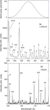 |
Fig. A.7. Spectrum of nickel in the range λ320–λ350: the spectrum in the middle panel was recorded with our moderate-resolution LoWEUS spectrograph at the EBIT-I electron beam ion trap at an electron beam energy of 1000 eV. Lines indicated by “2” are recognized as second diffraction order images. Fiducial markers indicate the rich structure of the spectrum, without being complete. Only the strongest of the known lines are identified by the spectrum number. The approximate band pass function of the SDO/AIA λ335 channel is indicated in the top panel. The lowest panel of the figure shows a high-resolution spectrum at half the wavelength and the strongest lines are identified by spectrum number. Strong first-diffraction order lines in this spectrum may appear in second diffraction order in the spectrum in the middle panel. |
Nickel lines observed in EBIT-I within the wavelength band λ320–λ350.
All Tables
Fluorine or sulfur lines observed in EBIT-I within the wavelength band λ320–λ350.
All Figures
|
Fig. A.1. Spectrum of carbon and oxygen in the range λ320–λ350: the spectrum in the middle panel was recorded using our moderate-resolution LoWEUS spectrograph at the EBIT-I electron beam ion trap at an electron beam energy of 700 eV. Identified spectral features are labeled by the corresponding spectrum. Several oxygen lines appear in second diffraction order (marked “2”). The lowest panel of the figure shows a high-resolution spectrum (from our HIGGS spectrograph) at half the wavelength. Strong first-diffraction order lines in this spectrum may appear in second diffraction order in the spectrum in the middle panel. The approximate band pass function of the SDO/AIA λ335 channel is indicated in the top panel. |
| In the text | |
|
Fig. A.2. Spectrum of nitrogen in the range λ320–λ350: the spectrum was recorded with our moderate-resolution LoWEUS spectrograph at the EBIT-I electron beam ion trap at an electron beam energy of 1000 eV. The line markers from fits to the data are visual aids only as the actual number of line components that in spectral line fits of blends can be discerned may depend on the available spectral resolution. Identified spectral features are labeled by the corresponding spectrum. Lines that are recognized as second diffraction order images are denoted “2”. The approximate band pass function of the SDO/AIA λ335 channel is indicated in the top panel. The second-diffraction order oxygen lines indicated are the same as in Fig. A.1, where a high-resolution measurement of these lines in first diffraction order is also shown. |
| In the text | |
|
Fig. A.3. Spectrum of fluorine and sulfur in the range λ320–λ350: the spectrum in the middle panel was recorded with our moderate-resolution LoWEUS spectrograph at the EBIT-I electron beam ion trap at an electron beam energy of 1000 eV. Visually recognized line positions are denoted. The lowest panel of the figure shows a high-resolution spectrum at half the wavelength, obtained using our HIGGS instrument. Strong first-diffraction order lines in this spectrum may appear in second diffraction order in the spectrum in the middle panel. Identified spectral features are labeled by the corresponding spectrum. We note the presence of several (known) O and F lines with wavelengths of 160 to 173 Å, the second diffraction order images (denoted “2”) of which appear in the range of the SDO/AIA λ335 band, but would not affect the observations with SDO/AIA. The approximate band pass function of the SDO/AIA λ335 channel is indicated in the top panel. |
| In the text | |
|
Fig. A.4. Spectrum of neon in the range λ320–λ350: the spectrum in the middle panel was recorded with our moderate-resolution LoWEUS spectrograph at the EBIT-I electron beam ion trap at an electron beam energy of 1000 eV. The approximate band pass function of the SDO/AIA λ335 channel is indicated in the top panel. Of the 59 lines seen in this spectrum (with eye-guiding markers), known second diffraction order images are denoted “2”. The lowest panel of the figure shows a high-resolution spectrum at half the wavelength. Strong first-diffraction order lines in this spectrum may appear in second diffraction order in the spectrum in the middle panel. |
| In the text | |
|
Fig. A.5. Spectrum of argon in the range λ320–λ350: the spectrum in the middle panel was recorded with our moderate-resolution LoWEUS spectrograph at the EBIT-I electron beam ion trap at an electron beam energy of 1000 eV. Eye-guiding markers indicate visual line positions. Known Ar lines are labeled by the spectrum number, while contamination lines from oxygen are labeled by the element. Lines that appear in second order of diffraction are denoted by “2”. The approximate band pass function of the SDO/AIA λ335 channel is indicated in the top panel. The lowest panel of the figure shows a high-resolution spectrum at half the wavelength. Strong first-diffraction order lines in this spectrum may appear in second diffraction order in the spectrum in the middle panel. |
| In the text | |
|
Fig. A.6. Spectrum of iron in the range λ320–λ350: the spectrum in the middle panel was recorded with our moderate-resolution LoWEUS spectrograph at the EBIT-I electron beam ion trap at an electron beam energy of 1000 eV. Fiducial markers indicate line positions as judged visually at this spectral resolution. The spectral features that arise from second diffraction order (denoted “2”) should not affect the SDO/AIA data. The approximate band pass function of the SDO/AIA λ335 channel is indicated in the top panel. The lowest panel shows a high-resolution spectrum at half the wavelength, in which the strongest lines and line groups are identified by spectrum number. Strong first-diffraction order lines in this spectrum may appear in second diffraction order in the spectrum in the middle panel. |
| In the text | |
|
Fig. A.7. Spectrum of nickel in the range λ320–λ350: the spectrum in the middle panel was recorded with our moderate-resolution LoWEUS spectrograph at the EBIT-I electron beam ion trap at an electron beam energy of 1000 eV. Lines indicated by “2” are recognized as second diffraction order images. Fiducial markers indicate the rich structure of the spectrum, without being complete. Only the strongest of the known lines are identified by the spectrum number. The approximate band pass function of the SDO/AIA λ335 channel is indicated in the top panel. The lowest panel of the figure shows a high-resolution spectrum at half the wavelength and the strongest lines are identified by spectrum number. Strong first-diffraction order lines in this spectrum may appear in second diffraction order in the spectrum in the middle panel. |
| In the text | |
Current usage metrics show cumulative count of Article Views (full-text article views including HTML views, PDF and ePub downloads, according to the available data) and Abstracts Views on Vision4Press platform.
Data correspond to usage on the plateform after 2015. The current usage metrics is available 48-96 hours after online publication and is updated daily on week days.
Initial download of the metrics may take a while.