| Issue |
A&A
Volume 617, September 2018
|
|
|---|---|---|
| Article Number | A107 | |
| Number of page(s) | 36 | |
| Section | Planets and planetary systems | |
| DOI | https://doi.org/10.1051/0004-6361/201832776 | |
| Published online | 26 September 2018 | |
Upper atmospheres of terrestrial planets: Carbon dioxide cooling and the Earth’s thermospheric evolution
1
University of Vienna, Department of Astrophysics,
Türkenschanzstrasse 17,
1180 Vienna,
Austria
e-mail: This email address is being protected from spambots. You need JavaScript enabled to view it.
2
Space Research Institute, Austrian Academy of Sciences,
Graz,
Austria
Received:
5
February
2018
Accepted:
18
June
2018
Abstract
Context. The thermal and chemical structures of the upper atmospheres of planets crucially influence losses to space and must be understood to constrain the effects of losses on atmospheric evolution.
Aims. We develop a 1D first-principles hydrodynamic atmosphere model that calculates atmospheric thermal and chemical structures for arbitrary planetary parameters, chemical compositions, and stellar inputs. We apply the model to study the reaction of the Earth’s upper atmosphere to large changes in the CO2 abundance and to changes in the input solar XUV field due to the Sun’s activity evolution from 3 Gyr in the past to 2.5 Gyr in the future.
Methods. For the thermal atmosphere structure, we considered heating from the absorption of stellar X-ray, UV, and IR radiation, heating from exothermic chemical reactions, electron heating from collisions with non-thermal photoelectrons, Joule heating, cooling from IR emission by several species, thermal conduction, and energy exchanges between the neutral, ion, and electron gases. For the chemical structure, we considered ~500 chemical reactions, including 56 photoreactions, eddy and molecular diffusion, and advection. In addition, we calculated the atmospheric structure by solving the hydrodynamic equations. To solve the equations in our model, we developed the Kompot code and have provided detailed descriptions of the numerical methods used in the appendices.
Results. We verify our model by calculating the structures of the upper atmospheres of the modern Earth and Venus. By varying the CO2 abundances at the lower boundary (65 km) of our Earth model, we show that the atmospheric thermal structure is significantly altered. Increasing the CO2 abundances leads to massive reduction in thermospheric temperature, contraction of the atmosphere, and reductions in the ion densities indicating that CO2 can significantly influence atmospheric erosion. Our models for the evolution of the Earth’s upper atmosphere indicate that the thermospheric structure has not changed significantly in the last 2 Gyr and is unlikely to change signficantly in the next few Gyr. The largest changes that we see take place between 3 and 2 Gyr ago, with even larger changes expected at even earlier times.
Key words: Earth / planets and satellites: atmospheres / planets and satellites: terrestrial planets / planet-star interactions / Sun: activity
© ESO 2018
1 Introduction
Planetary atmospheres evolve due to interactions with the planet’s surface and losses into space. At the surface, gas can be removed from the atmosphere by several processes, such as subduction (Marty & Dauphas 2003), and added to the atmosphere by other processes, such as outgassing during magma ocean solidification (Noack et al. 2014). At the top of the atmosphere, gases are lost to space, which over time can lead to significant atmospheric erosion (Lammer et al. 2014; Luger et al. 2015). Atmospheric loss into space takes place by a large number of different mechanisms (e.g. Lammer et al. 2008). One factor that is common to almost all of these processes is the fact that the loss rates depend strongly on the thermal and chemical structure of the upper atmosphere. Atmospheres that are hotter and more expanded have higher loss rates by essentially all mechanisms (e.g. Lichtenegger et al. 2010).
Much recent work has studied hydrodynamic losses of atmospheres. Many of these studies concentrate mostly on atmospheres composed primarily of H and He (e.g. Lammer et al. 2014; Shaikhislamov et al. 2014; Luger et al. 2015; Khodachenko et al. 2015; Owen & Mohanty 2016). Such atmospheres can experience very high hydrodynamic losses, largely due to the small average molecular masses of the gas (Erkaev et al. 2013). Atmospheres composed of water vapour, such as the possible early atmosphere of Venus, are also likely to undergo hydrodynamic escape as the dissociation of H2O creates large amounts of atomic H (Lichtenegger et al. 2016). Generally more interesting for planetary habitability are atmospheres dominated by heavier molecules, such as CO2, N2, and O2. The physical processes in these atmospheres are very complex (e.g. Kulikov et al. 2007; Tian et al. 2008a), and detailed models are needed to understand their structures. Such atmospheres are less likely to undergo hydrodynamic losses due to their higher molecular masses, and other atmospheric loss processes must be taken into account, such as polar ion outflows (Glocer et al. 2012; Airapetian et al. 2017) and pick-up of exospheric gas by the stellar wind (Kislyakova et al. 2014) and coronal mass ejections (Khodachenko et al. 2007; Lammer et al. 2007). In all cases, the specific atmospheric composition is critically important for the detailed physics of the upper atmosphere (Kulikov et al. 2007).
The most important input into the upper atmospheres of planets is the irradiation by the central star, especially in X-ray and ultraviolet (together XUV)1 wavelengths, though IR photons can also be important. The absorption causes dissociation and ionization, and significant heating. The energy gained by this heating is mostly lost by cooling due to IR emission from several molecules, most notably CO2. In the upper thermosphere of the Earth, the local heating is much stronger than the local cooling, and the excess energy is transported into the lower thermosphere by thermal conduction. The chemical structure of the upper atmosphere is determined by the composition of the lower atmosphere, chemical/photochemical reactions, and diffusion. Sophisticated models that take into account all of these processes have been applied for solar system planets for decades (e.g. Fox & Bougher 1991; Roble 1995; Ridley et al. 2006), but only a few studies have applied such models to planetary atmospheresunder very different conditions to those of the current solar system terrestrial planets (Tian et al. 2008a; Tian 2009).
The need for sophisticated first principles upper atmosphere models is clear when considering the range of atmospheric conditions that exist. In addition to different atmospheric compositions, the distribution of planets spans the entire range of possible masses and orbital distances from their host stars (López-Morales et al. 2016). Furthermore, different planets are exposed to very different conditions from the central star. Observations of young solar analogues have shown that the Sun was much more active in X-rays and UV than it currently is (Güdel et al. 1997; Ribas et al. 2005). Recently, Tu et al. (2015) showed that the early evolution of the Sun’s activity depended sensitively on its early rotation rate; this is important since we do not know how rapidly the Sun was rotating, and different evolutionary tracks for XUV can lead to different atmospheric evolution scenarios (Johnstone et al. 2015b). Stellar activity evolution depends also on the star’s mass, with lower mass stars remaining highly active for longer amounts of time (West et al. 2008). In addition, the exact shape of a star’s XUV spectrum depends on its spectral type and activity (Telleschi et al. 2005; Johnstone & Güdel 2015; Fontenla et al. 2016).
The aim of this paper is to develop and validate a first principles physical model for the upper atmospheres of planets and to apply it to the Earth to understand how the atmosphere reacts to changes in the CO2 abundances and the solar XUV spectrum. This physical model will be used as an important component in future studies on the evolution of terrestrial atmospheres. In Sect. 2, we present the complete physical model. In Sect. 3, we validate the model by calculating the atmospheric structures of Earth and Venus. In Sect. 4, we study the effects of enhanced CO2 abundances and the effects of the solar XUV evolution between 3 Gyr in the past and 2.5 Gyr in the future on the structure of the Earth’s upper atmosphere. In Sect. 5, we summarise and discuss our results. To solve the physical model presented in this paper, we have developed The Kompot Code, which we describe in the Appendices2. In the appendices, we describe in detail the numerical methods used to solve the equations described in Sect. 2.
2 Model
2.1 Model overview
The purpose of our model is to calculate the atmospheric properties as a function of altitude for arbitrary planetary atmospheres. The input parameters are the planetary mass and radius, the atmospheric properties at the base of the simulation, and the stellar radiation spectrum at the top of the atmosphere. Our computational domain is 1D and points radially outwards from the planet’s centre, extending between the lower boundary at an arbitrary altitude in the middle atmosphere to the upper boundary at the exobase. In the description of the state of the atmosphere, we make a few basic assumptions. Firstly, we assume that the gas has one bulk advection speed shared by the entire gas, though different chemical species have different diffusion speeds. Secondly, we assume that the neutrals, ions, and electrons have their own temperatures that evolve separately. Thirdly, we assume quasineutrality, meaning that the electron density is equal to the total ion density everywhere. The two stellar inputs are the XUV (i.e. X-ray and ultraviolet) field between 10 and 4000 Å, and the infrared field between 1 and 20 μm.
In this model, we break the gas down into components in two separate ways: in Eq. (1) the gas is broken down by different chemical species (e.g. N2, O2, CO2, etc.), and inEqs. (3)–(5), the gas is broken down into neutrals, ions, and electrons. In the rest of the paper, we define the “components” of the gas as the neutral, ion, and electron gases, and are referred to using the subscripts n, i, and e. Unless otherwise stated, when we discuss the electrons, we are referring to the thermal electron gas, and not the non-thermal electrons produced in photoionization reactions.
The main physical processes taken into account in this model are
atmospheric expansion/contraction in response to changes in the gas temperature and composition,
the transfer of X-ray, ultraviolet, and infrared radiation through the atmosphere, including the production of non-thermal electrons by photoionization reactions,
atmospheric chemistry, including photochemistry and reactions driven by impacts with non-thermal electrons,
molecular and eddy diffusion,
neutral heating by stellar XUV and IR radiation,
electron heating by impacts with non-thermal electrons,
infrared cooling, particularly by CO2 molecules,
heat conduction for each gas component,
-
and energy exchange between the components.
The equations that describe the changes of the atmosphere due to these processes are
![Mathematical equation: \begin{eqnarray}\frac{\partial n_j}{ \partial t} + \frac{1}{r^2} \frac{\partial \left[ r^2 ( n_j v + {\mathrm{\Phi}}_{\mathrm{d},j}) \right] }{\partial r} &=& S_j , \\[3pt]\frac{\partial ( \rho v ) }{ \partial t} + \frac{1}{r^2} \frac{\partial \left[ r^2 \left( \rho v^2 + p \right) \right] }{\partial r} &=& - \rho g + \frac{2 p }{r} ,\\[3pt]\small \frac{\partial e_{\mathrm{n}} }{ \partial t} + \frac{1}{r^2} \frac{\partial \left[ r^2 v \left( e_{\mathrm{n}} + p_{\mathrm{n}} \right) \right] }{\partial r} &=& - \rho_{\mathrm{n}} v g \left( Q_{\mathrm{h,n}} - Q_{\mathrm{c,n}} - Q_{\mathrm{in}} - Q_{\mathrm{en}} \right) \nonumber \\ && + \frac{1}{r^2} \frac{\partial}{\partial r} + \left[ r^2 \kappa_{\mathrm{mol}} \frac{\partial T_{\mathrm{n}}}{\partial r} \right. \nonumber \\ && \left. + r^2 \kappa_{\mathrm{eddy}} \left( \frac{\partial T_{\mathrm{n}}}{\partial r} + \frac{g}{c_{\mathrm{P}}} \right) \right] , \normalsize \\[3pt]\frac{\partial e_{\mathrm{i}} }{ \partial t} + \frac{1}{r^2} \frac{\partial \left[ r^2 v \left( e_{\mathrm{i}} + p_{\mathrm{i}} \right) \right] }{\partial r} &=& - \rho_{\mathrm{i}} v g + \left( Q_{\mathrm{h,i}} - Q_{\mathrm{c,i}} - Q_{\mathrm{ei}} + Q_{\mathrm{in}} \right) \nonumber \\* && + \frac{1}{r^2} \frac{\partial}{\partial r} \left[ r^2 \kappa_{\mathrm{i}} \frac{\partial T_{\mathrm{i}}}{\partial r} \right],\\[3pt]\frac{\partial e_{\mathrm{e}} }{ \partial t} + \frac{1}{r^2} \frac{\partial \left[ r^2 v \left( e_{\mathrm{e}} + p_{\mathrm{e}} \right) \right] }{\partial r} & = & - \rho_{\mathrm{e}} v g + \left( Q_{\mathrm{h,e}} - Q_{\mathrm{c,e}} + Q_{\mathrm{ei}} + Q_{\mathrm{en}} \right) \nonumber \\* && + \frac{1}{r^2} \frac{\partial}{\partial r} \left[ r^2 \kappa_{\mathrm{e}} \frac{\partial T_{\mathrm{e}}}{\partial r} \right], \end{eqnarray}](/articles/aa/full_html/2018/09/aa32776-18/aa32776-18-eq1.png)
where r is the radius, nj is the number density of the jth species, ρ is the total mass density, v is the bulk advection speed, ρv is the momentum density, ρk, ek, pk, and Tk are the mass density, energy density, thermal pressure, and temperature of the kth component of the gas, Φd,j and Sj are the diffusive particle flux and chemical source term of the jth species, g is the gravitational acceleration, Qh,k and Qc,k are the heating and cooling functions for the kth component, Qei, Qin, and Qen are the electron–ion, ion–neutral, and electron–neutral heat exchange functions, κmol and κeddy are the molecular and eddy thermal conductivities, κi and κe are the ion and electron thermal conductivities, and cP is the specific heat at constant pressure. Since chemistry and diffusion do not change the total mass density of the gas, Eq. (1) implies the standard mass continuity equation. It is also important at times to calculate γ (i.e. the ratio of specific heats) for the neutral and ion gases, which are mixtures of species with different γ values; for this we assume γj = 5∕3 for atomic species and γj = 7∕5 for molecular species3.
The exobaseis assumed to be where the mean-free-path of particles becomes larger than the pressure scale height. The mean free path is calculated from lmfp = 1∕(σN), where σ is the total collision cross-section, and N is the total number density. In reality, different species have different σ; however, the values tend to be similar and our calculated exobase location is not sensitive to small changes in σ. We therefore assume σ = 2 × 10⁻¹⁵ cm−2 always.
2.2 Hydrodynamics
Including gravity, the purely hydrodynamic parts of Eqs. (1)–(5) are
![Mathematical equation: \begin{eqnarray}&& \frac{\partial \rho}{ \partial t} + \frac{1}{r^2} \frac{\partial \left( r^2 \rho v \right) }{\partial r} = 0 , \\[7pt]&& \frac{\partial ( \rho v ) }{ \partial t} + \frac{1}{r^2} \frac{\partial \left[ r^2 \left( \rho v^2 + p \right) \right] }{\partial r} = - \rho g + \frac{2 p }{r} , \\[7pt]&& \frac{\partial e_{\mathrm{n}} }{ \partial t} + \frac{1}{r^2} \frac{\partial \left[ r^2 u \left( e_{\mathrm{n}} + p_{\mathrm{n}} \right) \right] }{\partial r} = - \rho_{\mathrm{n}} u g , \end{eqnarray}](/articles/aa/full_html/2018/09/aa32776-18/aa32776-18-eq2.png)
where the ion and electron energy equations are identical to the neutral energy equations with the n subscript replaced with the i and e subscripts. In Appendix B, we give an explicit method for solving these equations. Explicitly solving the full set of hydrodynamic equations is undesirable when the atmosphere is static, or close to static. We note that no atmosphere is ever fully hydrostatic since there is always some escape at the top of the atmosphere, meaning that there will always be a net upward flow of material.
In this paper, we use a method for solving the hydrodynamic equations given by Tian et al. (2008a). This method is not appropriate when the atmosphere is transonic, which is often the case for strongly irradiated planets. The basic simplifying assumption of the method is that the mass and momentum density structures are in a steady state, such that ∂ρ∕∂t = 0 and ∂(ρv)∕∂t = 0. Eqs. (6) and (7) can then be written
![Mathematical equation: \begin{eqnarray}&& 2 r \rho v + r^2 v \frac{{\rm{d}}\rho}{{\rm{d}}r} + r^2 \rho \frac{{\rm{d}}v}{{\rm{d}}r} = 0 , \\* [3pt]&& \frac{2 \rho v^2}{r} + 2 v \rho \frac{{\rm{d}}v}{{\rm{d}}r} + v^2 \frac{{\rm{d}}\rho}{{\rm{d}}r} + \frac{{\rm{d}}p}{{\rm{d}}r} = - \rho g. \vspace*{-3pt}\end{eqnarray}](/articles/aa/full_html/2018/09/aa32776-18/aa32776-18-eq3.png)
Assuming an ideal gas, the pressure is given by  and the radial derivative of p is
 (11)
(11)
where  and
and  and T are the average molecular mass and temperature of the entire gas. Putting these three equations together gives
![Mathematical equation: \begin{eqnarray}&& \frac{1}{v} \left( 1 - \frac{v^2}{v_0^2} \right) \frac{{\rm{d}}v}{{\rm{d}}r} = \frac{1}{T} \frac{{\rm{d}}T}{{\rm{d}}r} + \frac{g}{v_0^2} - \frac{1}{\bar{m}} \frac{{\rm{d}}\bar{m}}{{\rm{d}}r} - \frac{2}{r} , \\ [3pt]&& \frac{1}{\rho} \frac{{\rm{d}} \rho}{{\rm{d}}r} = - \frac{1}{T} \frac{{\rm{d}}T}{{\rm{d}}r} - \frac{g}{v_0^2} + \frac{1}{\bar{m}} \frac{{\rm{d}}\bar{m}}{{\rm{d}}r} - \frac{v}{v_0^2} \frac{{\rm{d}}v}{{\rm{d}}r}. \end{eqnarray}](/articles/aa/full_html/2018/09/aa32776-18/aa32776-18-eq8.png)
When v = 0, Eq. (13) gives the density structure of a hydrostatic atmosphere. As in Tian et al. (2008a), we solve these equations consecutively. Firstly, we update the energies using Eq. (8). With the new temperature structure and the already known structure of  , we then recalculate the structure of v by integrating from the exobase downwards through the grid using Eq. (12), assuming the outflow speed at the exobase is known. Finally, since the density at the lower boundary of the simulation is a fixed value and is therefore known, we calculate the structure of ρ by integrating upwards to the exobase using Eq. (13). For both the solution of the energy equations and the integration of ρ and v, we use the implicit Crank–Nicolson scheme, as described in Appendix D.
When the atmosphere is supersonic at the upper boundary, the material has escape velocity and simply flows away from the planet; in these cases, the appropriate boundary conditions are zero-gradient outflow conditions. Specifically, the values for each quantity in the final grid cell are made equal to the values in the second to last grid cell. When the atmosphere is subsonic at the upper boundary, we assume an outflow speed that is consistent with the Jeans escape rate. We first calculate the Jeans mass escape rate, ṀJeans, using the expressions given in Luger et al. (2015), and then calculate the upper boundary velocity from  .
.
When the bulk flow of the atmosphere is not negligible, the effects of advection on the species densities must be taken into account. We do this using the advection scheme described in Appendix B by converting the calculated cell boundary mass fluxes into individual species particle fluxes. When using the semi-static hydrodynamic approach, we use the advection scheme to calculate the mass fluxes only (i.e. Eqs. (B.11)–(B.18)). Since the total mass density structure is being calculated at every timestep assuming that it has already come to a steady state, the changes in the density are a result of advection that is not explicitly calculated in the model. To take this into account, after updating the structure of ρ using Eq. (13), we scale the species number densities by a species-independent factor at each location to ensure that ρ = ∑jmjnj, where the sum is over all species.
2.3 Stellar radiation and non-thermal electrons
2.3.1 X-ray and ultraviolet radiation
The most important external input into the upper atmosphere is the star’s X-ray and ultraviolet (=XUV) radiation. Its importance stems from the fact that atmospheric gases absorb radiation at XUV wavelengths very effectively. This means that the XUV radiation is absorbed high in the atmosphere where the gas densities are low and relatively small energy inputs can lead to large temperature changes. The XUV spectrum also drives the most important chemical processes in the upper atmosphere, and is therefore essential for calculating the chemical structure of the atmosphere.
We irradiate the atmosphere with a stellar XUV spectrum between 10 and 4000 Å. The XUV spectrum is divided into 1000 energy bins and represented by the irradiance, Iν, which is theenergy flux per unit frequency. This input spectrum is assumed to be unattenuated at the exobase. The radiation transfer through the atmosphere is then calculated based on the density structures of each absorbing species.
A weakness of 1D atmosphere models is that in reality the planet is being irradiated from one side only, which makes fully simulating the atmosphere at minimum a 2D problem. In 1D models, approximate simplifying assumptions must be made. We assume that the computational domain is pointing in an arbitrary direction relative to the position of the star. The angle between this direction and the direction that points directly at the star is the zenith angle, θ. We calculate the XUV spectrum at each point in the atmosphere by doing the radiation transfer from the exobase to each point separately. This geometry is demonstrating in Fig. 1, where the dashed black line shows the path that the radiation takes through the atmosphere. We assume that the state of the atmosphere at any given altitude is uniform over all latitudes and longitudes. This means that when doing the radiation transfer, we get the densities of each species at each given point by taking the values at the point in our simulation that has the same altitude. In all simulations in this paper, except our Venus simulation in Sect. 3.2, we assume a zenith angle of 66°. We find in Sect. 3.1 for the case of the Earth that this gives a decent representation of the atmosphere averaged over all longitudes and latitudes.
To calculate the XUV spectrum at a given grid cell, we integrate along the dashed black line in Fig. 1 for each energy bin using spatial stepswith length Δs given by H∕5, where H = N∕(dN∕dr) is the density scale height. The change in the irradiance over a path Δs is given by
 (14)
(14)
where Δτν is the optical depth along the path length Δs and is given by
![Mathematical equation: \begin{equation*}{\mathrm{\Delta}} \tau_{\nu} = {\mathrm{\Delta}} s \sum\limits_j \sigma_{\nu,j} [R_j] , \end{equation*}](/articles/aa/full_html/2018/09/aa32776-18/aa32776-18-eq12.png) (15)
(15)
where the sum is over all photoreactions in our chemical network, σν,j is the cross-section of the jth photoreaction at frequencyν, and [Rj] is the number density of the reactant in the jth photoreaction. By summing over individual photoreactions instead of using the total absorption cross-sections for each species, we ensure that the radiation transfer and the photochemistry are fully consistent. The individual photoreaction cross-sections are discussed in Sect. 2.4.1. In Fig. 2, we show the XUV spectrum at several altitudes in our model for the current Earth.
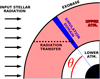 |
Fig. 1 Cartoon illustrating the geometry of the radiation transfer in our model. The bottom right of the cartoon is the centre of the planet and the incoming stellar radiation is travelling horizontally from left to right. The inner black region is the planet and the shaded region is the upper atmosphere. The simulation domain of our 1D atmosphere model, illustrated with the blue region, is a region that is pointing radially outwards from the planet centre. The angle θ is the zenithangle. To calculate the stellar XUV and IR spectra at any given point, we perform radiation transfer along the dashed black line. |
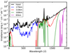 |
Fig. 2 Stellar XUV irradiance spectrum at different altitudes in the atmosphere of the Earth, calculated using our current Earth model presented in Sect. 3.1. The black and purple lines show the spectrum at the top and bottom of our model respectively. |
2.3.2 Infrared radiation
Another input into the atmosphere that can be important is the stellar infrared radiation. Although this has a negligible effect on the Earth’s upper atmosphere, it is a signficant source of heating for Mars and Venus (Bougher & Dickinson 1988; Fox & Bougher 1991). This difference is due to the different abundances of CO2, which is a strong absorber of IR radiation. We calculate the transfer of the stellar IR spectrum between 1 and 20 μm through the atmosphere, and its effect on atmospheric heating. For the input stellar IR spectrum, we assume a simple black-body spectrum with a temperature of 5777 K. We make the same geometrical assumptions for the IR radiation transfer as we make for the XUV, as demonstrated in Fig. 1, and perform the integration from the exobase to each grid cell using the same method described for XUV. For IR transfer, the sum in Eq. (15) for the optical depth is over all considered absorbing species, where σν,j and [Rj] are the cross-sections and number densities of the jth absorbing species. We consider only absorption of IR radiation by CO2 and H2O molecules. In future studies, the influences of other molecules will be included when necessary.
We calculate the absorption spectra of CO2 and H2O using the software package kspectrum (Eymet et al. 2016), which is an open-source code for calculating the high resolution absorption spectra of common atmospheric gases using the HITRAN 2008 and HITEMP 2010 molecular spectroscopic databases (Rothman et al. 2009; Rothman et al. 2010). Although the absorption spectrum is temperature and pressure dependent, we calculate the cross-sections at 200 K and 10−2 mbar only and use these values everywhere in the atmosphere. In order to resolve all features in the CO2 absorption spectrum, a large number (~106) of spectral bins are needed. The wavelength-dependent absorption cross-sections for CO2 and H2 O are shown in Fig. 3. However, including so many energy bins is computationally too expensive for our model; instead, we only consider energy bins that have cross-sections above 10−22 cm2 for at least one of the considered molecules. Tests have shown that we get identical results using this threshold, while limiting the number of energy bins to something reasonable (~ 104).
The heating of the atmosphere by the absorption of IR radiation is discussed in Sect. 2.5.1. We calculate the heating assuming that all energy removed from the radiation field by absorbtion is immediately added to the thermal energy reservoir of the neutral gas. What actually happens is that the absorption of photons excites the molecules and the heating of the gas only takes place when they are then collisionally deexcited. Some of this energy will not in fact end up in heat, but will be reradiated back into space. To take this into account, we add an additional excitation term into the equations for 15 μm CO2 cooling in Sect. 2.5.2. We write the excitation rate due to stellar IR photons as
![Mathematical equation: \begin{equation*}S_{\mathrm{IR}} = \frac{ \int\limits_{\nu} \sigma_{\nu,\mathrm{co}_2} [\mathrm{CO}_2] I_{\nu} {\rm{d}}\nu }{ (h\nu)_{15\mu \mathrm{m} } }, \end{equation*}](/articles/aa/full_html/2018/09/aa32776-18/aa32776-18-eq13.png) (16)
(16)
where the integral is over all considered frequencies,  and [CO2] are the absorption cross-section and number density of CO2 at frequency ν, and
  is the energy of a 15 μm photon. The cgs units for SIR are excitations s−1 cm−3. The numerator in Eq. (16) gives the volumetric heating rate due to the absorbtion of IR photons by CO2. The assumption here is that all energy absorbed from the IR field by CO2 eventually contributes to the excitation ofthe 15 μm bending mode in CO2 molecules. The main absorption bands are at 15, 4.3, 2.7, and 2.0 μm. The latter two are combination bands, and photons absorbed in these bands cause multiple excitations in the 15 and 4.3 μm band transitions. Our assumption in Eq. (16) is reasonable if the majority of energy in the 4.3 μm vibrational state is transferred to the 15 μm vibrational state by vibrational–vibrational exchanges, as argued by Taylor & Bitterman (1969; see the discussion in Sect. 2 of Dickinson 1976).
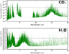 |
Fig. 3 Infrared absorption spectra of CO2 (upper panel) and H2O (lower panel) as calculated by kspectrum (Eymet et al. 2016). The gas is assumed to have a temperature of 200 K and a pressure of 10−2 mbar. The horizontal dashed line shows the cross-section of 10−22 cm−3. |
2.3.3 Non-thermal electrons
Many of thephotoionization reactions that take place in the upper atmosphere are caused by photons that contain significantly more energythan is needed simply to cause the ionization. This additional energy is given to the produced photoelectrons in the form of kinetic energy, which results in a population of photoelectrons that have significantly larger energies than the thermal energy of the electron gas. These high energy photoelectrons then lose their energy by collisions with other atmospheric particles. For the thermal electrons, elastic collisions with non-thermal electrons is the main heat source and is the reason why the electron gas becomes hotter than the neutral and ion gases in the Earth’s upper thermosphere (Smithtro & Solomon 2008).
The two main assumptions in our model are that the photoelectrons lose their energy locally where they are created and that the non-thermal electron spectrum is in a steady state at each point. Given the latter assumption, the spectrum can be calculated simply by balancing sources and sinks of electrons at each electron energy. In future models, we will include also a more sophisticated electron transport model; this was shown to influence the heat deposition by Tian et al. (2008b). For the effects of collisions, the situation is complicated by the fact that a given atmospheric species can interact with a non-thermal electron in multiple ways. Each of these different interactions has a different energy-dependent cross-section and takes a different amount of energy from the impacting electron.
At a given electron energy, Ee, the two sources of electrons are photoionization reactions producing electrons with energy Ee, and the degradation of more energetic electrons through collisions with the ambient gas. The production spectrum for photoelectrons by photoionization reactions, Pe(E), is given by
![Mathematical equation: \begin{equation*}P_{\mathrm{e}} (E_{\mathrm{e}}) = \sum\limits_k \frac{ I_{\mathrm{xuv}} (E_{\mathrm{e}} + \delta E_k) }{E_{\mathrm{e}}+\delta E_k} \sigma_k (E_{\mathrm{e}} + \delta E_k) [R_k] , \end{equation*}](/articles/aa/full_html/2018/09/aa32776-18/aa32776-18-eq16.png) (17)
(17)
where the sum is over all photoionization reactions considered, σk (Ee) is the energy dependent cross-section for the kth photoionization reaction, [Rk] is the number density of the reactant in the kth photoionization reaction, and δEk is the energy required for the ionization to take place. We calculate the non-thermal electron spectrum using
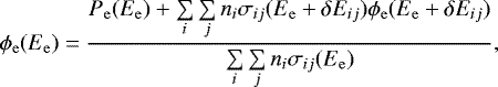 (18)
(18)
where ϕe(Ee) is the electron flux at energy Ee and σij is the cross-sections for electron impact interactions. This expression is described in more detail by Schunk & Nagy (1978). In both the numerator and the denominator, the first sum is over all species that the electrons interact with and the second sum is over all possible interactions with that species. The second term in the numerator is the source term from the degradation of higher energy electrons. The fact that photoelectrons can only lose energy, so that ϕe at a given energy depends on the higher energies values of ϕe only, makes solving Eq. (18) trivial. To do this, we break the spectrum down into 100 discreetenergy bins logarithmically spaced between 1 and 1000 eV. We first calculate ϕe at the bin with the highest energy assuming ϕe = 0 for higher energies, and then iterate downwards through the spectrum, calculating ϕe in each bin.
The neutral interacting species that we consider are N2, O2, O, CO2, CO, and He. For N2, we use the electron impact cross-sections given in Green & Barth (1965). For non-ionising O2 transitions, we use the cross-sections from Watson et al. (1967), and for O2 ionizations we use cross-sections from Jackman et al. (1977). For O, CO2, and CO, we use cross-sections from Jackman et al. (1977). For He, we use cross-sections from Jusick et al. (1967).
In Fig. 4 we show our predicted non-thermal electron spectrum up to 70 eV for the current Earth’s atmosphere at an altitude of 200 km. This spectrum is an output of the Earth model presented in Sect. 3.1. For comparison, we also show the spectra calculated for several altitudes by Singhal & Haider (1984), which they compared to other models and observations in their Fig. 3. Our spectrum match theirs well for almost the entire energy range, indicating that our model calculates approximately realistic non-thermal electron spectra.
In our chemical network, we have included several ionization reactions due to impacts with non-thermal electrons. For each of these reactions, the total cross-sections for use in Eq. (21) are calculated by summing over the cross-sections for each corresponding ionization interaction. For many of the transitions that are not direct ionizations, an ionization can still take place by autoionization. We take these into account when calculating the total ionization cross-sections for O, CO2, and CO by multiplying the cross-sections for these transitions by the autoionization factors given by Jackman et al. (1977). These reactions also remove energy from non-thermal photoelectrons, but the situation is complicated since the products of these reactions include two electrons. The energy of the original non-thermal electron that is not used to cause the reaction is distributed between the two electrons. For simplicity, we assume that one of the electrons gets this energy, and the other just becomes a normal thermal electron.
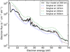 |
Fig. 4 Our prediction for the non-thermal electron spectrum at 200 km for the current Earth. For comparison, the dashed lines show the spectra at several altitudes calculated by Singhal & Haider (1984; taken from their Fig. 3 and multiplied by 4πto move the sr−1 from the units). The sudden increase in the flux at low electron energies is due to the thermal electron spectrum becoming dominant. |
2.4 Chemical structure of the atmosphere
2.4.1 Chemistry
In this study, we attempt to construct a general chemical network that can be applied to a range of atmospheres with arbitrary compositions. This is difficult given the huge numbers of reactions and species that any network could consider and the uncertainties in the rate coefficients for the reactions, particularly at high temperatures. We do this by combining the networks of several previously published atmospheric models. The networks that we use are from Fox & Sung (2001), Verronen et al. (2002, 2005), Yelle (2004), García Muñoz (2007), Tian et al. (2008a), Richards & Voglozin (2011), Fox (2015), and Fox et al. (2015). We include almost all reactions from these papers, with some reactions being excluded if they introduced species that we consider unimportant. The rate coefficients are taken also from these studies in almost every case. Where multiple papers give different rate coefficients for the same reaction, we take the values almost arbitrarily, or find the coefficients on the KIDA database (Wakelam et al. 2012). In addition, we add a few reactions from KIDA that are not in any of these networks when necessary to stop reactions from creating species that are not destroyed. For the photoreactions, we take all of the relevant reactions from the PHIDRATES database (Huebner & Mukherjee 2015), which provides wavelength dependent cross-sections for the entire XUV spectrum. These cross-sections are all temperature independent, which is in many cases unrealistic and could lead to inaccuracies in our photochemistry (Venot et al. 2018). The few reactions involving non-thermal electrons produced in photoionization reactions are described in Sect. 2.3.3. The resulting network, which is given in Appendix H, contains 63 species, including 30 ion species, and 503 reactions, including 56 photoreactions and 7 photoelectron reactions.
The reaction rate of the kth chemical reaction, Rk, is related to the rate coefficient, kk, by
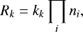 (19)
(19)
where the RHS gives the product of the densities of all reactants. The rate coefficients for normal reactions are typically functions of temperature and many of the reactions have temperature limits, both of which are listed in Table H.1. A difficulty in our model is that we calculate separate neutral, ion, and electron temperatures, and in many cases it is unclear which of these temperatures to use to calculate the rate coefficients. For reactions that have only neutral reactants, we use the neutral temperature; for reactions that have a mixture of neutrals, ions, and electrons as reactants, we simply use the averages of the temperatures of the involved components (e.g. if a reaction has one neutral reactant and one ion reactant, we set Tgas = (Tn + Ti)∕2 in the equation for the rate coefficient). For photoreactions, the rate coefficients depend on the XUV spectrum and the wavelength dependent cross-sections by
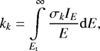 (20)
(20)
where E is the photon energy, Et is the threshold energy for the reaction, σk is the cross-section, and IE is the irradience in units of energy flux per unitenergy (the quantity Iν used elsewhere in this paper is the irradience in units of energy flux per unit frequency). Similarly, the equation for the rate coefficients of reactions involving inelastic collisions with non-thermal electrons is
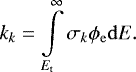 (21)
(21)
The result is a set of ordinary differential equations, one for each species, describing the rates of change of the species densities. For the jth species, this can be written
 (22)
(22)
where the first sum is over all reactions that create the jth species, and the second sum is over all reactions that destroy it. The Sj term is the total source term for the jth species in the RHS of Eq. (1). To evolve nj using Eq. (22), we use an implicit Rosenbrock solver described in Appendix H.
In our model, we break the gas down into neutral, ion, and electron components. A difficulty in our model is that the chemical reactions cause the transfer of mass, momentum, and energy between the components simply due to the changes in the identities of atoms and molecules. For example, consider the reaction N+ + O2 → NO+ + O; this reaction transfers an O atom from the neutral gas to the ion gas. The changes in the mass and momentum densities of the components are trivial to calculate, but the changes in the energy densities are not. We avoid this problem by assuming that the temperatures are unaffected when updating the species densities due to chemistry. The heating of the gas due to exothermic and endothermic chemical reactions, and the energy exchanges between the neutral, ion, and electron gases, are calculated separately, as described in Sect. 2.5.
2.4.2 Diffusion
Many of thespecies considered in the simulation are created and destroyed slowly by chemical and photochemical reactions. For these species, a very important transport mechanism is diffusion. Our model takes into account both molecular and eddy diffusion. Eddy diffusion evolves the density profiles so that they all follow the pressure scale height of the entire gas; molecular diffusion evolves the density profiles so that they all follow their own pressure scale heights. In the homosphere, eddy diffusion dominates and the mixing ratios of the long-lived species are independent of altitude. In the heterosphere, molecular diffusion dominates and the densities of heavy species decrease with increasing altitude faster than the densities of light species, meaning that light species become increasingly dominant at higher altitudes (this also happens due to the dissociation of heavy molecules). The equation that we use for the diffusive flux of the jth species, including both eddy and molecular diffusion, is
 (23)
(23)
where vd,j is the diffusion speed, given by
![Mathematical equation: \begin{equation*}\begin{aligned} v_{\mathrm{d},j} = & - D_j \left[ \frac{1}{n_j} \frac{{\rm{d}}n_j}{{\rm{d}}r} - \frac{1}{N} \frac{{\rm{d}}N}{{\rm{d}}r} + \left( 1 - \frac{m_j}{\bar{m}} \right) \frac{1}{p} \frac{{\rm{d}}p}{{\rm{d}}r} + \frac{\alpha_{\mathrm{T},j}}{T} \frac{{\rm{d}}T}{{\rm{d}}r} \right] \\ & - K_{\mathrm{E}} \left[ \frac{1}{n_j} \frac{{\rm{d}}n_j}{{\rm{d}}r} -\frac{1}{N} \frac{{\rm{d}}N}{{\rm{d}}r} \right] , \end{aligned} \end{equation*}](/articles/aa/full_html/2018/09/aa32776-18/aa32776-18-eq23.png) (24)
(24)
where Dj and KE are the molecular and eddy diffusion coefficients, nj and N are the particle number densities of the jth species and of the entire gas, mj and  are the molecular masses of the jth species and of the entire gas, p and T are the thermal pressure and temperatureof the entire gas, and αT,j is the thermal diffusion factor. To solve these equations, we use the implicit Crank–Nicolson method described in Appendix E.
For molecular diffusion, the diffusion coefficient for a given species, Dj, depends on both the species itself, the composition of the background gas, and the temperature. For all diffusion coefficients, we use the relation
 (25)
(25)
For H, H2, He, CH4, CO, Ar, CO2, and O, we use values for αj and sj given in Tables 15.1 and 15.2 of Banks & Kockarts (1973) assuming an N2 background atmosphere, which is likely reasonable since the values are very similar for the other background atmospheres. For simplicity, we assume αj = 1 and sj = 0.75 for all other species. For H, H2, and He, we assume αT,j = −0.38 and for Ar, we assume αT,j = 0.17 (Banks & Kockarts 1973); for all other species, we assume αT,j = 0.
In models such as ours, the eddy diffusion coefficients as a function of altitude are free parameters; this is the only free parameter in our model. We assume it is given by KE = ANB, where KE and N have the units cm2 s−1 and cm−3 respectively. This functional form is typically used for models of Venus and Mars (von Zahn et al. 1980; Fox & Sung 2001). For Venus, we use A = 2 × 10¹³ and B = −0.5 and impose a maximum value for KE of 6 × 108 cm2 s−1. These values were used by Fox (2015) for the upper atmosphere of Mars, and are very similar to values found for Venus (von Zahn et al. 1980). For the current Earth, we first fit A and B to the tabulated KE values givenby Roble (1995), but we scale these values up by a factor of ten in order to fit the expected O2 densities at high altitudes in our Earth model. This gives A = 108 and B = −0.1. We note that even without scaling up the eddy diffusion coefficients from Roble (1995), we obtain good fits to the density profiles of all other species.
For atmospheres that are close to hydrostatic, it is important to specify a diffusion flux at the exobase. We assume an outward diffusion flux that corresponds to Jeans escape. This is only necessary for the lightest species (H and He), so for all species more massive than 4 mp, we assume a zero flux. In simulations where the gas at the exobase is supersonic, and therefore is faster than the escape velocity, we simply assume a zero diffusion flux at the exobase.
2.5 Thermal structure of the atmosphere
2.5.1 Heating
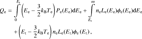
In this model, the important energy sources are stellar XUV (10–4000 Å) and IR (1–20 μm) radiation. We also include a simple treatment of Joule heating. The total energy deposition rate from a radiation field travelling a distance dx through an absorbing gas is − dF∕dx, where F is the energy flux (=∫ Iνdν). In reality, the absorbed energy is not directly added to the thermal energy budget of the gas, and not all of the energy deposited is eventually converted to heat. A common way to calculate the heating is to multiply the total energy deposition rate by a heating efficiency factor (e.g. Erkaev et al. 2013; Johnstone et al. 2015b); this assumption is generally undesirable since it adds an unconstrained free parameter into the model. We instead use a more complete heating model where the energy release from different processes are calculated individually. The heating processes considered are direct heating by the stellar XUV field, electron heating by elastic collisions with non-thermal electrons, heating from exothermic chemical reactions, direct heating by the stellar IR field, and Joule heating. A diagram demonstrated how stellar XUV energy in our model is transferred to heat after been absorbed is shown in Fig. 5.
When a XUV photon is absorbed, a large part of its energy is used to cause either a dissociation, an ionization, or both. For photodissociation reactions, the remaining photon energy is given to the products as kinetic energy, and ultimately dissipated as heat in the gas. It is this heating that we consider the direct heating by the stellar XUV field. To calculate this direct heating, we need to consider each photodissociation reaction and each energy bin in the XUV field separately. The full equation for the heating rateis
 (26)
(26)
where Qxuv,k is the heating rate by the kth reaction and is given by
![Mathematical equation: \begin{equation*} Q_{\mathrm{xuv,k}} = \int\limits_{E_{\mathrm{T},k}}^{\infty} \left( E - E_{\mathrm{T},k} \right) \frac{I_E}{E} \sigma_k (E) [R_k] {\rm{d}}E , \end{equation*}](/articles/aa/full_html/2018/09/aa32776-18/aa32776-18-eq27.png) (27)
(27)
where the sum is over all photodissociation reactions, ET,k is the energy required for the reaction to take place, σk(E) is the reaction cross-section at energy E, [Rk] is the number density of the reactant, and IE is the irradience in units of energy flux per unit energy. The term IE ∕E is the photon flux per unit photon energy at energy E and the term (IE∕E)σk(E)[Rk] is the rate at which the kth reaction takes place per unit volume per unit photon energy. The energy released per reaction is E− ET,k, which when multipled by the reaction rate and integrated over all photon energies gives the heating rate for the kth reaction.
For photoionization reactions, we do not give the remaining photon energy to the gas as heat directly, but instead assume that all this energy is given to the resulting free electron and we calculate the non-thermal electron spectrum, as described in Sect. 2.3.3. This energy is either given to the neutral gas by inelastic collisions, typically exciting atoms/molecules or causing secondary ionizations, or it is given to the thermal electrons by elastic collisions. We assume that the energy given to the neutral gas is all lost by radiative relaxation and consider therefore only the heating of the electron gas. Using the expression given by Schunk & Nagy (1978), we calculate the electron heating rate as
 (28)
(28)
where Ee is the electron kinetic energy, Pe(Ee) is the production spectrum of electrons (see Eq. (17)), Et is the energy above which the non-thermal flux is larger than the thermal flux, and Le (Ee) is the loss function given by
 (29)
(29)
where Eth = 8.618 × 10⁻⁵ Te (Swartz et al. 1971). The three terms on the RHS of Eq. (28) give respectively the heating/cooling by the direct production of thermal electrons by photoionization reactions, heating of thermal electrons by elastic collisions with non-thermal electrons, and a surface term related to the crossover between the thermal and non-thermal electron spectra. Although a more accurate version of the surface term was derived by Hoegy (1984), we use the version given above because it is simpler and is sufficiently accurate for our purposes.
Much of the photon energy used to cause a photoreaction is not lost, but is instead converted into chemical potential energy that can then be released as heat in exothermic chemical reactions. The heating rate at a given point by chemical reactions is given by
 (30)
(30)
where the sum is over all chemical reactions, and Rk and Qchem,k are the reaction rate and energy released per reaction for the kth reaction. The values of Qchem,k are given for each reaction in Table H.1. These energies are mostly taken from Tian et al. (2008a) or from the KIDA database, and when the energy for a given reaction is not available in either of these sources, we simply assume it does not contribute to the heating.
We consider also heating of the atmosphere by the abosrption of IR radiation. We assume that all of the energy removed from the IR spectrum is input into the neutral gas as thermal energy, giving a heating rate of
![Mathematical equation: \begin{equation*}Q_{\mathrm{IR}} = \sum\limits_j \int\limits_{\nu} \sigma_{\nu,j} [R_j] I_{\nu} {\rm{d}}\nu, \end{equation*}](/articles/aa/full_html/2018/09/aa32776-18/aa32776-18-eq31.png) (31)
(31)
where the sum is over all absorbing species, the integral is over the entire IR spectrum that we consider, and σν,j and [Rj] are the absorption cross-section and number density of the jth absorbing species. In reality, this energy is first used to excite CO2 and is then released as heat through collisional deexcitation, which we take into account with an additional excitation term in the equations for CO2 cooling.
Additionally, the upper atmospheres of magnetised planets are heated by two magnetospheric processes: these are energetic particle precipitation and Joule heating. For the Earth, during quiet geomagnetic conditions these two processes are likely similar in magnitude, and Joule heating tends to dominate during geomagnetic storms (e.g. Chappell 2016). This process could become important for planets that are exposed to extreme space weather (Cohen et al. 2014). Both processes are most significant at high latitudes, but tend not to influence the global heat budget significantly during quiet conditions. In this paper, we model Joule heating using the simplified model described in Roble et al. (1987) and Smithtro & Sojka (2005). The two input parameters are the ambient magnetic field strength, which we assume is 0.5 G everywhere, and the total global Joule heating rate, which we assume is 1.4 × 10¹⁸ erg s−1. This is double the value used in Roble et al. (1987), which is typical for quiet levels of geomagnetic activity (Foster et al. 1983); we double the value to take into account also the energy input expected from particle precipitation. We calculate the heating rate at each altitude using
 (32)
(32)
where E is the electric field strength and σP is the Pedersen conductivity (Foster et al. 1983). We do not calculate the electric field, but instead assume that it is a constant and use it as a free parameter that can be scaled in order to give us the desired total global Joule heating rate. The Pedersen conductivity varies with altitude, and at a given point depends on the densities of individual ion and neutral species, the gas temperature, and the ambient magnetic field strength. The σP profiles are calculated self-consistently within the model using the equations described in Sect. 5.11 of Schunk & Nagy (2000). The equation for σP is
 (33)
(33)
where the sum is over all considered ion species, and σi, νi, and ωi are the ion conductivity, ion-neutral collision frequency, and angular gyrofrequency of the ith ion species. The angular gyrofrequency is given by ωi = qiB∕mi. The ion conductivity is given by 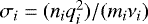 , where ni, qi, and mi are the ion number density, charge, and mass respectively. The ion-neutral collision frequency, νi, is calculated as the sum over the collision frequencies with individual neutral species, such that
  , where νin is the frequency of collisions between the ith ion species and the nth neutral species. For this, we use the same collisions and νin values described in Sect. 2.5.4 for ion-neutral heat exchange.
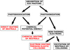 |
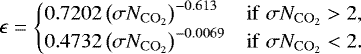
Fig. 5 Simplified cartoon illustrating the main pathways taken in our model by the energy that is removed from the XUV field by absorption due to photodissociation and photoionization reactions. In both cases, much of the energy used to cause the photoreaction is released due to exothermic chemical reactions. For photodissociation, the remaining energy from the absorbed photon is given to the thermal energy budget of the neutral gas directly. For photoionization, the remaining energy is released as kinetic energy of the produced electron, and is then lost as the electron collides with the ambient gas; collisions with neutral species are inelastic and lead to excitation, dissociation, and ionization, whereas collisions with ambient thermal electrons are elastic and lead to heating of the electron gas. |
2.5.2 Cooling
We consider the effects of IR cooling by CO2, H2 O, NO, and O. In all cases, cooling happens when atoms/molecules are excited by collisions with other particles and then radiate the energy awaybefore they are deexcited by further collisions. Collisions cause there to be a continuous transfer of energy from the atmosphere’s thermal energy reservoir to the various forms of energy within the individual atoms and molecules, and a corresponding transfer of energy back to the thermal energy reservoir. However, due to radiative relaxation (i.e. spontaneous/stimulated emission) and the loss of many of the emitted photons to space, the rate at which energy is transferred back to the thermal reservoir is reduced, and the resulting inbalance is the cooling that we are interested in. The calculation of the cooling rates is seldom trivial and ideally would involve calculating the full transport ofthe emitted IR spectrum through the atmosphere and tracking the populations of each of the various excited states in the relevant species (e.g. see Wintersteiner et al. 1992). In this paper, we take into account all of these processes in a simpler way and aim to implement more sophisticated treatments of cooling in future studies.
Cooling by CO2 is dominated by emission at 15 μm. We use the cool-to-space approximation (e.g. Dickinson 1972); the fundamental assumption is that the cooling at each point is caused entirely by emitted photons that escape directly to space. Ignoring stimulated emission, this means
![Mathematical equation: \begin{equation*}Q_{\mathrm{CO}_2} = (h\nu)_{15\mu \mathrm{m} } A_{10} [ \mathrm{CO}_2^* ] \epsilon , \end{equation*}](/articles/aa/full_html/2018/09/aa32776-18/aa32776-18-eq36.png) (34)
(34)
where  is the energy of a single 15 μm photon (=1.325 × 10⁻¹³ erg), A10 is the Einstein coefficient for spontaneous emission,
 ![Mathematical equation: $[ \mathrm{CO}_2^* ]$](/articles/aa/full_html/2018/09/aa32776-18/aa32776-18-eq38.png) is the density of excited CO2 molecules, and ϵ is the probability that a 15 μm photon emitted from a given point escapes to space. The definition of ϵ is such that it takes into account the fact that photons emitted downwards are not lost, and therefore approaches a maximum of 0.5 at high altitudes.
is the density of excited CO2 molecules, and ϵ is the probability that a 15 μm photon emitted from a given point escapes to space. The definition of ϵ is such that it takes into account the fact that photons emitted downwards are not lost, and therefore approaches a maximum of 0.5 at high altitudes.
In order to calculate ![Mathematical equation: $[ \mathrm{CO}_2^* ]$](/articles/aa/full_html/2018/09/aa32776-18/aa32776-18-eq39.png) , we consider three excitation and two deexcitation mechanisms. The excitation mechanisms are collisional excitation, the absorption of 15 μm photons previously emitted by excited CO2 molecules, and the absorption of photons from the host star’s IR spectrum. For the second process, the fundamental simplifying assumption is that all photons that are emitted and are not lost to space are reabsorbed locally where the emission took place. The excitation rate is given by
, we consider three excitation and two deexcitation mechanisms. The excitation mechanisms are collisional excitation, the absorption of 15 μm photons previously emitted by excited CO2 molecules, and the absorption of photons from the host star’s IR spectrum. For the second process, the fundamental simplifying assumption is that all photons that are emitted and are not lost to space are reabsorbed locally where the emission took place. The excitation rate is given by
![Mathematical equation: \begin{eqnarray*}\frac{ {\rm{d}} [\mathrm{CO}_2^*] }{ {\rm{d}}t } &=& \left( \sum\limits_M k_{e,M} [M] \right) \left( [\mathrm{CO}_2] - [\mathrm{CO}_2^*] \right) \nonumber \\ & & + A_{10} [ \mathrm{CO}_2^* ] \left( 1 - \epsilon \right) + S_{\mathrm{IR}} , \end{eqnarray*}](/articles/aa/full_html/2018/09/aa32776-18/aa32776-18-eq40.png) (35)
(35)
where the sum is over all species that collisionally excite CO2, ke,M is the rate coefficient for collisional excitation, and SIR is the additional excitation term due to the absorption of stellar IR radiation given by Eq. (16). The term ![Mathematical equation: $[\mathrm{CO}_2] - [\mathrm{CO}_2^*]$](/articles/aa/full_html/2018/09/aa32776-18/aa32776-18-eq41.png) is the density of non-excited CO2 molecules. The deexcitation mechanisms are collisional deexcitation and radiative relaxation. The deexcitation rate is given by
is the density of non-excited CO2 molecules. The deexcitation mechanisms are collisional deexcitation and radiative relaxation. The deexcitation rate is given by
![Mathematical equation: \begin{equation*}- \frac{ {\rm{d}} [\mathrm{CO}_2^*] }{ {\rm{d}}t } = \left( \sum\limits_M k_{d,M} [M] \right) [\mathrm{CO}_2^*] + A_{10} [ \mathrm{CO}_2^* ] . \end{equation*}](/articles/aa/full_html/2018/09/aa32776-18/aa32776-18-eq42.png) (36)
(36)
Where the first term on the RHS dominates, the atmosphere is in the local thermodynamic equilibrium (LTE) regime, and where the two terms are similar, or the second term dominates, the atmosphere is in the non-local thermodynamic equilibrium (non-LTE) regime. Assuming a steady state, Eqs. (35) and (36) add up to zero, giving
![Mathematical equation: \begin{equation*}\left[ \mathrm{CO}_2^* \right] = \frac{ \sum\limits_M k_{e,M} [M] [\mathrm{CO}_2] + S_{\mathrm{IR}} }{ \sum\limits_M \left( k_{e,M} + k_{d,M} \right) [M] + A_{10} \epsilon } . \end{equation*}](/articles/aa/full_html/2018/09/aa32776-18/aa32776-18-eq43.png) (37)
(37)
The Einstein coefficient, A10, is 0.46 s−1 (Curtis & Goody 1956), and the rate coefficients are related by  (Castle et al. 2006). For the escape probabilities, we use the tabulated values given by Kumer & James (1974) which depend entirely on the amount of CO2 above the considered altitude, z, given by
 ![Mathematical equation: $N_{\mathrm{CO}_2} = \int_z^{\infty} [\mathrm{CO}_2] {\rm{d}}z$](/articles/aa/full_html/2018/09/aa32776-18/aa32776-18-eq45.png) . We fit their tabulated values with
. We fit their tabulated values with
 (38)
(38)
where σ =6.43 × 10⁻¹⁵ cm2. The dependence of ϵ on  is shown in Fig. 6. For the collisional excitation/deexcitation rate, we consider the influences of O, O2, N2, CO2, He, and Ar. For O, we use the experimentally measured values of kd,M given by Castle et al. (2012), and for the other species, we use the measured values given by Siddles et al. (1994). In all cases, kd,M have temperature dependences that we fit using power-laws of the form
 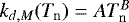 , where the values of A and B are given in Table 1. In Fig. 6, we show the measured deexcitation rates and our analytic fit formulae for each species. A signficant worry with our fit formulae for kd,M is that all of the measurements that we use are for low gas temperatures, and therefore our fit formulae might be inaccurate at high temperatures. This problem is not likely to influence our results in this paper since CO2 cooling is only significant in regions of the atmospheres that are within the experimental temperature ranges.
For NO cooling, we use the model given by Oberheide et al. (2013). We consider emission in the vibrational band at 5.3 μm assuming two excitation mechanisms: these are collisional excitation by O atoms and radiative pumping by earthshine. We assume that all photons emitted by NO molecules escape to space (i.e. ϵ = 1), which is realistic for the Earth since NO cooling is only significant in the thermosphere (Kockarts 1980). The cooling rate is given by
![Mathematical equation: \begin{equation*}Q_{\mathrm{NO}} = (h\nu)_{5.3\mu \mathrm{m} } A_{10} [ \mathrm{NO}^* ] , \end{equation*}](/articles/aa/full_html/2018/09/aa32776-18/aa32776-18-eq49.png) (39)
(39)
where  erg and [NO*] is the density of excited NO molecules, given by
![Mathematical equation: \begin{equation*}[ \mathrm{NO}^* ] = \frac{ k_{e,\textrm{O}} [\textrm{O}] + S_{\mathrm{E}} }{ \left( k_{e,\textrm{O}} + k_{d,\textrm{O}} \right) [\textrm{O}] + S_{\mathrm{E}} + A } [\mathrm{NO}], \vspace*{2pt}\end{equation*}](/articles/aa/full_html/2018/09/aa32776-18/aa32776-18-eq51.png) (40)
(40)
where SE is the excitation rate due to earthshine, ke,O and kd,O are the collisional excitation and deexcitation rate coefficients, and A is the Einstein coefficient for spontaneous emission. As in Oberheide et al. (2013), we use SE = 1.06 × 10⁻⁴ s−1, kd,O = 2.8 × 10⁻¹¹ cm3 s−1, A =12.54 s−1, and  .
.
For O cooling, we consider emission at 63 μm and 147 μm using the parameterization derived by Bates (1951; see Eqs. (14.57) and (14.58) of Banks & Kockarts 1973) given by
 (41)
(41)
where
![Mathematical equation: \begin{eqnarray}&& Q_{\mathrm{O},63\mu\mathrm{m}} = \frac{ 1.67 \times 10^{-18} \exp\left( -228/T_{\mathrm{n}} \right) [\mathrm{O}] }{ 1 + 0.6 \exp\left( -228/T_{\mathrm{n}} \right) + 0.2 \exp\left( -326/T_{\mathrm{n}} \right) }, \\ [4pt]&& Q_{\mathrm{O},147\mu\mathrm{m}} = \frac{ 4.59 \times 10^{-20} \exp\left( -326/T_{\mathrm{n}} \right) [\mathrm{O}] }{ 1 + 0.6 \exp\left( -228/T_{\mathrm{n}} \right) + 0.2 \exp\left( -326/T_{\mathrm{n}} \right) }, \end{eqnarray}](/articles/aa/full_html/2018/09/aa32776-18/aa32776-18-eq54.png)
where [O] is in cm−3, Tn is in K, and the cooling rates are in erg s−1 cm−3. More sophisticated modelling of O cooling will be used in future models.
For cooling by H2O, we use the parametitzation for emission in rotational bands by Hollenbach & McKee (1979) and summarised in Kasting & Pollack (1983, see their Eqs. (32)–(38)). In this model, H2 O is excited by collisions with H atoms only. Given the length of the set of equations involved, we do not write them here.
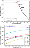 |
Fig. 6 Escape probability of a 15 μm photon as a function of CO2 optical depth (upper panel) and the CO2 deexcitation rate coefficients as a function of temperature (lower panel). In the upper panel, the numbers show the approximate altitudes in our current Earth model where these points on the line are reached. In the lower panel, the data points are measurements from Siddles et al. (1994) and Castle et al. (2012), and the solid lines are our power-law fits, given in Table 1. |
2.5.3 Conduction
In the Earth’s upper thermosphere, cooling of the neutral gas is not strong enough to balance heating, and a steady state is only reached because conduction downwards into the cooler lower thermosphere removes this excess energy. Since the temperatures of the neutrals, ions, and electrons are evolved separately, separate conductivities must be used for each of these components. For ion and electronconductivities, we ignore the effects of the magnetic field, which reduces the conduction in directions perpendicular to the magnetic field. The conduction equations are solved using the implicit Crank–Nicolson method, as described in Appendix F.
For the neutral gas, we consider eddy conduction, which is dominant in the lower atmosphere, and molecular conduction, which is dominant in the upper atmosphere. The neutral conduction equation is
![Mathematical equation: \begin{equation*}\frac{\partial e_{\mathrm{n}}}{\partial t} = \frac{1}{r^2} \frac{\partial}{\partial r} \left[ r^2 \kappa_{\mathrm{mol}} \frac{\partial T_{\mathrm{n}}}{\partial r} + r^2 \kappa_{\mathrm{eddy}} \left( \frac{\partial T_{\mathrm{n}}}{\partial r} + \frac{g}{c_{\mathrm{P}}} \right) \right] , \end{equation*}](/articles/aa/full_html/2018/09/aa32776-18/aa32776-18-eq55.png) (44)
(44)
where κmol is the molecular conductivity, κeddy is the eddy conductivity, g is the gravitational acceleration, and cP is the specific heat at constant pressure. The term g∕cP for the eddyconduction is the adiabatic lapse rate. The eddy conductivity is related to the eddy diffusion coefficient by κeddy = ρcPKE (Hunten 1974). The molecular conductivity is dependent on the temperature and composition of the gas. We estimate κmol using the equations given in Sect. 14.3 of Banks & Kockarts (1973) with some minor simplifications. The molecular conductivity of the kth species is given by
 (45)
(45)
where Ak and sk are coefficients that depend on the species. We assume the total conductivity of the gas is given by
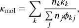 (46)
(46)
where
![Mathematical equation: \begin{equation*}\phi_{kj} = \frac{ \left[ 1 + \left( \kappa_k / \kappa_j \right)^{\frac{1}{2}} \left( m_j / m_k \right)^{\frac{1}{4}} \right]^2 }{ 2 \sqrt{2} \left[ 1 + \left( m_j / m_k \right) \right]^{\frac{1}{2}} } , \end{equation*}](/articles/aa/full_html/2018/09/aa32776-18/aa32776-18-eq58.png) (47)
(47)
where mk is the molecular mass of the kth species. Thesums in Eq. (46) should be over all neutral species, but in reality we only consider species for which we have Ak and sk values. The species we consider are N2, O2, CO2, CO, O, He, H, and Ar, with values for Ak and sk taken from Table 13 of Bauer & Lammer (2004) for Ar, and Table 10.1 of Schunk & Nagy (2000) for the others.
For the ions, the conduction equation is
![Mathematical equation: \begin{equation*}\frac{\partial e_{\mathrm{i}}}{\partial t} = \frac{1}{r^2} \frac{\partial}{\partial r} \left[ r^2 \kappa_{\mathrm{i}} \frac{\partial T_{\mathrm{i}}}{\partial r} \right], \end{equation*}](/articles/aa/full_html/2018/09/aa32776-18/aa32776-18-eq59.png) (48)
(48)
where κi is the ion conductivity. For κi, we use Eq. (22.122) from Banks & Kockarts (1973) which expresses the conductivity of ion gases made of a single ion species as  eV cm−1 s−1 K−1, where A is the atomic mass of the species and Ti is the ion temperature. For a gas mixture, they recommend using a density weighted average thermal conductivity, so we adopt the form
 (49)
(49)
where the sums are over all ion species and nk is in cm−3, Ti is the ion temperature in K, and κi is in eV cm−1 s−1 K−1.
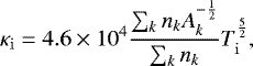
For the thermal electron gas, the conduction equation is the same as Eq. (48) with the subscript i replaced by e. We calculate the electron conductivity using Eq. (22.116) of Banks & Kockarts (1973):
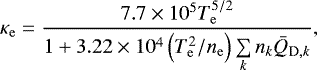 (50)
(50)
where  is the average momentum transfer cross-section of the kth species. The sum in the denominator should technically be over all neutral species, but in reality only the main species contribute significantly. In this sum, we take into account the effects of N2, O2, O, H, and He using the temperaturedependent equations for
  given in Table 9.2 of Banks & Kockarts (1973). The numerator in Eq. (50) is the electron conductivity of a fully ionised gas, and the denominator corrects for the reduction in conductivity caused by collisions with neutrals reducing the mean free paths of thermal electrons.
2.5.4 Energy exchange
The neutral, ion, and electron gases exchange energy by collisions. In our model, the electrons lose energy only by collisions with neutrals and ions. The energy gained by the ions is then given to the neutrals by further collisions, which is the most important neutral heating mechanism in the upper thermosphere. The energy exchange equations are solved using the implicit Crank–Nicolson method, as described in Appendix G.
For the electron-ion energy exchange, we take into account elastic Coulomb collisions only and the total energy exchange rate is calculated by summing over the rates for individual ion species. The basic equation is
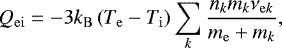 (51)
(51)
where the sum is over all ion species and νek is the momentum transfer collision frequency between electrons and the kth ion species, This equation, derived by Schunk (1975), requires several assumptions, including that the temperature difference between the electrons and ions are small. The definition of Qei is such that a positive value means energy is taken from the ions and given to the electrons. To calculate νe k for a given ion, we use νe k = 54.5  , where Zk is the charge of the ion (see Sect. 4.8 of Schunk & Nagy 2000).
The total ion-neutral energy exchange rate is the sum of the exchange rates of individual species pairs. The equation for the energy exchange rate is
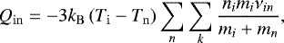 (52)
(52)
where the subscripts n and i are for the nth neutral and ith ion species. The definition of Qin is such that a positive value means energy is taken from the neutrals and given to the ions. The neutrals that we consider in the sums are H, He, N, O, CO, N2, O2, and CO2; the ions that we consider are H+, He+, C+, N+, O+, CO+, N , NO+, O
 , and CO
 . The ion-neutral heat exchange, described in detail in Schunk & Nagy (2000), is dominated by two types of interactions: resonant and non-resonant interactions which dominate at high (>300 K) and low temperatures respectively. The resonant interactions happen when a neutral approaches its ion equivalent (e.g. O and O+) and charge exchanges with it, with the changing identities of the particles representing a net energy exchange between the ion and neutral gases. We use the temperature-dependent equations for the momentum transfer collision frequencies, νin, for individual ion-neutral pairs given in Table 4.5 of Schunk & Nagy (2000). Non-resonant interactions involve neutral species and dissimilar ions. For these interactions, νin can be described simply by νin = Cinnn, where we use the coefficients Cin for individual ion-neutral pairs given in Table 4.4 of Schunk & Nagy (2000).
Several important mechanisms exist that cause thermal electrons to lose energy to the neutral gas. Electron–neutral heat exchange is very important for the electron temperature structure in the low thermosphere of the Earth, and normally proceeds through inelastic collisions that excite neutral atoms or molecules. The most important of these processes, at least for the current Earth, is inelastic collisions that cause fine structure transitions in ground state atomic oxygen; for this process, we use the scaling laws derived by Hoegy (1976). We also consider the excitation of ground state oxygen to the O(1 D) excited state. In addition, we take into account energy exchange from electron collisions with neutral molecules that cause the exitation of rotational or vibrational modes in the molecule; for these, we consider collisions with N2, O2, H2, CO2, CO, and H2O. We use the scaling laws for these processes that are convieniently listed in Sect. 9.7 of Schunk & Nagy (2000).
3 Model validation
To validate our model, we calculate the upper atmospheres of modern Earth and Venus in this section. In both simulations, we use the modern solar XUV spectrum given by Claire et al. (2012), which represents the Sun approximately at the maximum of its activity cycle.
3.1 Earth
To validate our model for the Earth, we compare our results to those of two empirical models. For the neutral gas, we use the atmospheric density and temperature profiles of the empirical NRLMSISE-00 model (Picone et al. 2002). This model produces vertical profiles for the Earth’s atmosphere at arbitrary longitudes and latitudes and at arbitrary dates; the output profiles that we use are for temperature, and the densities of N2, O2, N, O, H, Ar, and He. For the ion densities, we use International Reference Ionosphere 2007 (IRI-2007; Bilitza & Reinisch 2008). This model produces vertical profiles for O , NO+, O+, N+, H+, and electrons. We use these two standard models to obtain vertical atmospheric profiles for all longitudes and latitudes on the 1st January 1990, when the Sun was at approximately peak activity. We then calculate globally averaged profiles for this date. For our own Earth simulation, we assume a zenith angle of 66°, which we show below provides a good approximation for the globally averaged profiles.
We model the Earth’s upper atmosphere between an altitude of 65 km and the exobase. At the lower boundary, we use the values for temperature and density from this altitude in the NRLMSISE-00 model for comparison purposes, and additionally assume CO2 and H2 O mixing ratios of 4 × 10⁻⁴ and 6 × 10⁻⁶ respectively, which are reasonable values for the Earth’s middle atmosphere (Körner & Sonnemann 2001). In Fig. 7, we show the thermal structure of our current Earth model. The dashed line shows the standard atmosphere model that we use for comparison for the neutral gas temperature. The comparison between our results and the standard atmosphere model is very good, though an exact match between the models should not be expected especially since our input solar XUV spectrum will not match exactly the one used to produce the standard model. In Fig. 8, we show the strengths of the various heating and cooling mechanisms for this model. The results resemble very closely those of other global upper atmosphere models (e.g. Roble 1995; Tian et al. 2008a).
In Fig. 9, we show the densities as a function of altitude of several important species in our simulation. The species are chosen to be those output by the NRLMSISE-00 and IRI-2007 models that we use for comparison. Our predicted density structures are very similar to those of the comparison models, with the only exception being He, which we predict to be less abundant at high altitudes than expected. Clearly our model is able to realistically predict the structure of the Earth’s atmosphere.
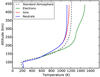 |
Fig. 7 Neutral, ion, and electron temperature structures of our current Earth model. The dashed black line is for the empirical NRLMSISE-00 model. |
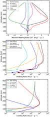 |
Fig. 8 Thermal processes in our Earth model as functions of altitude. In the upper panel, the red line shows the total XUV, chemical, and Joule heating, the blue line shows the total IR cooling, the cyan and magenta lines show the neutral heating by collisions with electron and ions, the black line shows the sum of all of these, and the green line shows the effects conduction. In the middle and lower panels, we show the contributions of individual mechanisms to the total heating and cooling. |
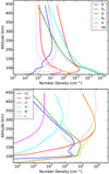 |
Fig. 9 Density structures of several important neutral (upper panel) and ion (lower panel) species. The solid lines show the predictions of our model and the dotted lines are from the empirical NRLMSISE-00 model for the neutrals and the IRI-2007 model for the ions. |
3.2 Venus
In this section, we further validate our model by calculating the structure of the upper atmosphere of Venus. This is especially useful since Venus’ atmosphere is made up mostly of CO2 and has therefore much stronger atmospheric cooling, allowing us to test that our model realistically responds to large changes in the CO2 content. For a reference atmosphere, we use the empirical thermosphere model given in Table 3b of Hedin et al. (1983), which is for Venus’ atmosphere at noon during approximately solar maximum conditions. We therefore assume a zenith angle of 0° in our model and use the values given by Hedin et al. (1983) for the temperature and species densities at the lower boundary. We do not include Joule heating in our Venus model.
In Fig. 10, we show a summary of the results of our Venus model. We compare our calculated temperature structures to the standard model given by Hedin et al. (1983) and to the recent 3D global models for the full atmosphere of Venus by Gilli et al. (2017). The neutral temperature profile resembles that of Hedin et al. (1983), with very similar exobase temperatures, though we find that our model is colder in the lower thermosphere, with the largest difference being around 40 K around 130 km. These differences in the temperature profiles do not suggest that there is a problem with our simulations; the Gilli et al. (2017) model is also colder than the Hedin et al. (1983) profiles at 140 km, though it is much warmer than both our model and the Hedin et al. (1983) lower in the thermosphere. In Fig. 10, the density profiles for several species from our simulations can be compared to those from Hedin et al. (1983). As with the case of the Earth’s thermosphere, we underestimate the He abundances at high altitudes. Our other density profiles are similar to those of Hedin et al. (1983), with the differences being mostly due to the different temperatures.
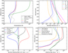 |
Fig. 10 Results of our modern Venus model. In the upper left panel, showing the temperature profiles, the dashed black line shows the empirical model by Hedin et al. (1983) and the dotted black line shows the daytime profiles shown in Fig. 9 of Gilli et al. (2017). In the upper right panel, showing the density profiles of several important species, the solid lines show the results of our model and the dotted lines show the profiles given by Hedin et al. (1983). The lower left panel shows the heating and cooling mechanisms for the neutral gas, and the lower right panel shows all of the heating mechanisms. |
4 Results
We present two applications of our code. In Sect. 4.1, we explore the effects of enhancing the CO2 abundance in the current Earth’s atmosphere on the upper atmospheric structure. In Sect. 4.2, we explore the response of Earth’s upper atmosphere to the evolving XUV spectrum of the Sun.
4.1 The influence of enhanced CO2 abundance on the atmospheric structure
To study the response of the Earth’s upper atmosphere to large changes in the CO2 abundance, we calculate several models for the current Earth, varying only the lower boundary density of CO2. We calculate models where the CO2 base density is 0.01, 0.1, 1, 10, 100, and 1000 times the value for the current Earth. We refer to these models by this multiplicative factor, such that our model with 1000 times more CO2 is the 1000× model. In our 1000× model, CO2 has a mixing ratio of approximately 0.3, which is a factor of a few lower than that of Venus. As in previous sections, our input solar spectrum is for the current Sun at activity maximum.
It is important to note that the fact that we do not include the effects of changing the CO2 abundances on the lower atmosphere. In reality, large changes in the CO2 abundances will cause also changes in these lower boundary properties. This has the effect that the total heating and cooling rates approximately balance only in our 1× model. In models with lower CO2 abundances, energy is removed from the computational domain at the lower boundary by downward conduction, causing the total cooling to be less than the total heating. In models with higher CO2 abundances, the opposite effect takes place.
In Fig. 11, we show the neutral temperature structures for each model. As expected, increasing the CO2 abundance leads to a significant decrease in the thermospheric temperature due to enhanced CO2 cooling. Similarly, decreasing the amount of CO2 leads to the thermosphere becoming hotter. In the 1000 × model, the maximum temperature reached in the thermosphere is only ~300 K, similar to that of Venus, and the mesosphere is cooled to a minimum temperature of ~130 K, which is much cooler than the minimum temperature of ~200 K that we find in our current Earth model. Fig. 11 also shows the total atmospheric heating rate4 as a function of CO2 mixing ratio for different heating processes. We note however that these quantities are relatively crude measures of how important the various heating mechanisms are; for example, the total photoelectron heating for the current Earth is very small, but the effect is relatively large because it takes place high in the thermosphere where the gas densities are low and therefore less energy is required for the heating to be significant.
In the current Earth case, the two dominant heating mechanisms are chemical and XUV heating. These two mechanisms depend primarily on the input XUV energy flux, and therefore remain approximately constant. Due to the decrease in the ionization fraction of the gas, the heating of the electrons by collisions with non-thermal photoelectrons decreases significantly as the CO2 mixing ratio is increased (see the linear dependence between electron heating and density in Eq. (28)). The mechanism that changes the most is the heating due to the absorption of stellar IR photons. Unlike the stellar XUV photons, which are all absorbed in the upper atmosphere in all cases, most of the IR photons pass through the upper atmosphere unhindered; therefore, adding efficient IR absorbing gases influences significantly how much IR energy is absorbed. In the 1000× model, we find that most of the heating is from IR absorption, especially at low altitudes. In the 0.01× model, the IR heating is dominated by H2O absorption.
It is interesting to compare our simulations to those of Kulikov et al. (2007) who also modelled the effects on enhanced CO2 abundances on the Earth’s thermosphere (see their Fig. 2). Our results are broadly similar which provides additional validation of our model. We find in general cooler upper thermospheric temperatures than they do for the enhanced CO2 models. Our models differ in a few important ways: for example, they did not calculate separate neutral, ion, and electron temperatures and they did not consider the effects of chemical reactions on the density structures of individual species. The differences between our results likely have two sources. Firstly, the XUV heating in their model is based on an assumed heating efficiency parameter that in reality might vary with CO2 abundance. Secondly, they put the lower boundaries of their models at the mesopause at an altitude of 100 km with an approximately fixed temperature, whereas we calculate the upper mesosphere from 65 km. In the enhanced CO2 models, we get significant additional mesospheric cooling, and therefore much lower mesopause temperatures, which leads to cooler temperatures also at higher altitudes.
The changes in the exobase are demonstrated in Fig. 12. In the models with larger CO2 abundances, the exobase altitudes and gas temperatures are much lower. Interestingly, the electron temperature does not decrease as much as the neutral and ion temperatures. This is largely because the total photoionization rate is approximately the same in all of our atmosphere models, meaning that the amount of energy in the non-thermal electron spectrum is also approximately constant. The volumetric heating rate for electrons is lower in simulations with higher CO2 abundances because the electron densities are lower, but the heating rate per electron is in fact higher.
The lower panel in Fig. 12 shows the mixing ratios of several important species at the exobase as a function of CO2 abundance, including the total ion mixing ratio. The exobase composition changes significantly, especially for N2 and O2; although O remains the most abundant species at the exobase in all simulations, in the 1000× simulation, the N2 mixing ratio is similar to that of O. The changes in the exobase N2 and O2 mixing ratios are primarily because of the change in the exobase altitude. As the atmosphere cools and the exobase moves to lower altitudes, the molecular diffusion rates and the distance between the homopause and the exobase are reduced, giving molecular diffusion less of a chance to separate the heavier and lighter species.
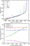 |
Fig. 11 Neutral temperature structures for our simulations with different base mixing ratios of CO2 (upper-panel) and the total atmospheric heating rates due to the various heating processes as a function of CO2 mixing ratio (lower-panel). In the upper panel, the lines (which stop at the exobase) are simulations where the base CO2 density is 0.01, 0.1, 1, 10, 100, and 1000 times the value for the current Earth, which has a mixing ratio at 65 km of 4 × 10⁻⁴. |
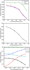 |
Fig. 12 Temperatures (upper panel), altitudes (middle panel), and mixing ratios of several important species of the exobase (lower panel) as a function of the CO2 mixing ratio at 65 km. In the lower panel, the black line gives the total ion mixing ratio (i.e. the ionization fraction). |
4.2 The evolution of Earth’s upper atmosphere
In this section, we explore the responses of the upper atmospheres of Earth to the evolving XUV spectrum of the Sun between 3 Gyr in the past and 2.5 Gyr in the future. We do not consider the effects of the evolving lower atmospheric composition, which we will study in future work. We use the XUV spectra from Claire et al. (2012), who produced solar spectra as a function of age for all wavelengths that are of interest to us. We note that at young ages, the XUV spectra of solar mass stars are not unique functions of age given that they follow different rotational and activity evolution tracks (Johnstone et al. 2015a), which can be very important for the evolution of a planet’s atmosphere (Johnstone et al. 2015b). Since we do not know how rapidly the Sun was rotating at young ages, we do not know its early XUV output (Tu et al. 2015). However, at the ages that we consider, the rotation rates of young solar mass stars have converged to unique age dependent values, and so the unique XUV evolution presented by Claire et al. (2012) is valid.
In Fig. 13, we show our results for the Earth. In the upper-left panel, the temperature structures for our models at several ages are shown; the lines in this panel can be seen as an evolutionary sequence from right to left, with the thermospheres becoming cooler and less extended as the Sun’s XUV spectrum decays. In all cases, the neutral and ion temperatures are approximately the same at all altitudes and the electron temperatures are higher. In the upper-right panel, the evolutions of the exobase temperatures are shown. Interestingly, the electron temperatures at the exobase are higher by approximately the same amount (i.e. ~500 K) at all ages. At 3 Gyr ago, our models suggest that the exobase neutral and electron temperatures were approximately 4600 and 5100 K respectively. Our models also suggest that going into the future, we should not expect a large change in the upper atmosphere of the Earth simply due to the Sun’s activity decay. This is consistent with the power-law dependence of the solar activity on age, which means that the fastest changes take place at young ages; in our models, the atmosphere changes the most between 3 and 2 Gyr ago, and all changes after that are relatively slow in comparison.
Our results for the temperature structures are broadly consistent with those calculated by Tian et al. (2008a). Since Claire et al. (2012) used a more realistic method for estimating the spectra of the Sun at higher activity levels, we should not expect any exact agreement between our models and those of Tian et al. (2008a) even for the same total input XUV flux. Our model for 3 Gyr in the past corresponds approximately to their model with input fluxes of 4.9 times the current solar value, and we get similar results. Although not studied in this paper, in models withan even more active Sun, we can also see the effects of adiabatic cooling that were found by Tian et al. (2008a).
The middle row of Fig. 13 shows the exobase altitude and composition. The largest change in the altitude of the exobase takes place between 3 and 2 Gyr ago, dropping from 2000 km to approximately 600 km in that time. This is mostly due to the decrease in the thermospheric temperature, but is also partly due to the change in the chemical composition of the gas. At the youngest age considered, we find that the chemical composition at the exobase contains much more N and much less N2 than we find for the current Earth, though O is in all cases the dominant species. Interestingly, we do not find any change in the exobase mixing ratios of H and He, which stay at values of ~ 5 × 10⁻⁵ at all ages. The ionization fraction at the exobase also decreases with age by about an order of magnitude between 3 Gyr ago and now.
Since the atmospheres are never fully hydrodynamic in our simulations, the dominant mass loss rates are likely to be non-thermal processes. Calculating these requires the application of additional models, which we do not attempt in this paper. We can calculate from our models the Jeans escape rates, which are shown for several species in the lower panels of Fig. 13. For the current Earth, it is well known that the only species undergoing significant Jeans escape is H, due to its low molecular mass. As we go to the past however, the Jeans escape rates of He, O, and N increase significantly, and in our earliest model are within approximately two orders of magnitude of the escape rate of H. If we were to go further into the past, the Jeans escape rates of these species would become comparable to that of H; it is around this time that we would find the atmosphere becoming hydrodynamic and the effects of adiabatic cooling on the temperature structures becoming important.
It is interesting to consider how the various heating mechanisms evolve with the evolving solar spectrum. In Fig. 14, we show the evolutions of direct XUV heating, chemical heating, and photoelectron heating for three altitude ranges. The quantities are the volumetric heating rates integrated over all the relevant altitudes and normalised to the modern Earth values. For altitudes above 100 km, the total heating rates for all these processes decrease with age due to the decreasing solar magnetic activity. However, at lower altitudes, the heating rates in fact increase with age. This is because this heating comes almost entirely from O3 absorption at wavelengths longer than 2000 Å, which is generated in the solar photosphere. Since the Sun’s bolometric luminosity is increasing as it ages, the heating in the lower atmosphere of the Earth also increases. We note that the heating in the lower regions of our model should in fact be lower at young ages due to the absence of O2 in the atmosphere prior to the Great Oxidation Event. The largest change is seen for heating of thermal electrons by non-thermalphotoelectrons, which we find was around 14 times larger 3 Gyr ago than the modern value. This is a result of the higher photoionization rates leading to there being more energy in the photoelectron spectrum and the greater ionization fractions of the gas leading to a larger fraction of that energy being transferred to the thermal electrons through elastic collisions, as opposed to being transferred to the neutrals through inelastic collisions.
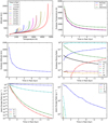 |
Fig. 13 Our simulation results for the response of the Earth’s atmosphere to the evolving XUV spectrum of the Sun. In the upper left panel, we show the temperature structures for several of these models, where the different colours are for different ages and the solid, dashed, and dotted lines show the neutral, ion, and electron temperatures respectively. In all cases, the lines end at the exobase. In the upper right, middle left, and middle right panels, we show the exobase temperatures, altitudes, and chemical compositions as functions of age. In the lower left and lower right panels, we show the evolution of Jeans escape for H, O, N, and He, with the difference between the two plots being the range on the y-axis. In each figure, the small circles show the exact locations of each simulation. |
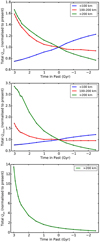 |
Fig. 14 Evolution of direct XUV heating (upper panel), chemical heating (middle panel), and photoelectron heating (lower panel) within three altitude ranges in the Earth’s atmosphere. The quantities plotted are the total heating rates integrated over the relevant volumes and normalised to the values for the modern Earth. For photoelectron heating, only the values for altitudesbetween 200 km and the exobase are shown since at lower altitudes this process is negligible. |
5 Discussion
In this paper, we develop and validate a physical model for the thermal and chemical structures of planetary upper atmospheres. We use this model to estimate how the Earth’s upper atmosphere would look if the CO2 abundance was varied by a large amount, and to explore the response of the upper atmosphere to the evolving XUV spectrum of the Sun. Increasing the CO2 abundance causes the Earth’s upper atmosphere to be much cooler and contracted, presumably causing a dramatic decrease in atmospheric losses. This could also be important for the evolution of the Earth’s atmosphere since without some form of protection, such as the enhanced CO2 abundances expected during earlier epochs (Zahnle et al. 2010), interactions with the solar wind could have stripped away the early Earth’s atmosphere (Lichtenegger et al. 2010). This is also important because, based on the examples of Venus, Mars, and likely the early Earth, CO2 dominated atmospheres are likely common among terrestrial exoplanets.
Our physical model should be applicable to a range of situations with arbitrary atmospheric compositions and stellar input XUV and IR spectra. For this purpose, we have attempted to develop the model in such a way that, as much as possible, it is based on first-principles physics. This means that we have avoided adding free parameters in our model, and we rely as little as possible on parametrised scaling laws that have been developed for the solar system terrestrial planets. For example, our model does not rely on parametarised heating efficiencies, but instead it calculates the heating rates for each of the contributing physical mechanisms explicitly. However, our model still contains several weaknesses; for example, our treatment IR cooling should be improved with more detailed treatment of radiation transfer and the detailed interactions between the IR field and the various coolants.
The main reason that we are interested in the thermal and chemical structures of the atmospheres of terrestrial planets is their importance for atmospheric losses into space. Even just for the case of the Earth, the atmosphere has radically changed many times, especially in the first billion years after the Earth’s formation. Models such as ours are essential tools for understanding this diverse set of atmospheric conditions. Estimating atmospheric loss rates atmospheres would require additional detailed modelling of the planetary exospheres (e.g. Kislyakova et al. 2013) and of the interactions of the ionosphere with the planet’s magnetic field (e.g. Glocer et al. 2009), which we do not attempt in this paper. In future work, we will combine the model developed in this paper with other such models to gain a more complete understanding of how losses to space influence atmospheric evolution.
Acknowledgments
The authors thank the anonymous referee for useful comments on our manuscript. This study was carried out with thesupport by the FWF NFN project S11601-N16 “Pathways to Habitability: From Disk to Active Stars, Planets and Life” and the related subprojects S11604-N16, and S11607-N16. We also acknowledge the support by grant 16-52-14006 of the Russian Fund of Basic Research, and the Austrian Science Foundation (FWF) projects I2939-N27, S11606-N16.
Appendix A The Kompot code
To solve the physical model described above, we have developed The Kompot Code, which calculates the 1D thermal and chemical structure of a planet’s atmosphere. The underlying equations for the physical model are described in Sect. 2, and the numerical methods used to solve these equations are described in the following appendices. The code is designed to be very flexible, such that it can be applied to a wide range of atmospheres, and the underlying physics can be easily modified and improved. The physical input parameters into the code are the temperature and species densities at the lower boundary, and the stellar XUV and IR spectra at the exobase. It is written in Fortran and Python and has been parallelised using OpenMP. The Kompot Code will be made publicly available in the near future and will be obtainable by contacting the authors.
Evolving the state of the atmosphere forward in time using the system of equations described in Sect. 2 is not trivial since they contain many terms that are different in form. For example, consider Eq. (1) in the following form:-
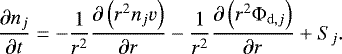 (A.1)
(A.1)
The first term on the RHS is for advection and contains a ∂nj ∕∂r term. The second term is for diffusion and contains multiple ∂2nj∕∂r2 terms. The third term describes the chemical sources and is a stiff system of many ordinary differential equations. No one numerical method is ideally suited to solve all of these problems simultaneously. We instead use operator splitting to solve each one sequentially using different numerical methods.
The simulation takes place on a finite static spatial grid of cells and we calculate all quantities at cell centres. For accuracy and efficiency we place our cells in such a way that the cell spacing increases linearly with altitude. The code only considers the cells below the exobase, the location of which varies within the simulation.
The initial conditions of a simulation should be irrelevant for the final result, but this is only the case when they are not too unrealistic. We have three ways to calculate the initial conditions. Firstly, we can start the simulation assuming hydrostatic equilibrium, a uniform temperature, and uniform mixing ratios for all species. For numerical reasons, it is often necessary to evolve the initial chemical structure of the atmosphere by an arbitrary amount of time before starting the simulation, mostly to avoid starting with no ions and electrons in the gas. Secondly, we can start many simulations simply using the atmospheric structure from the results of previous simulations. Thirdly, in fully hydrodynamic simulations, we start the simulation assuming an isothermal Parker wind structure and uniform chemical composition.
We evolve the atmosphere forward in time by performing a large number of timesteps, with length Δ t. We determine Δt by multiplying the minimum time taken for a sound wave to cross one grid cell by a fixed number, called the Courant number, C. Unless we are applying the full hydrodynamic method given in Appendix B, our simulations are not strictly constrained by the Courant Friedrichs Lewy condition that C should be less than unity, though we often assume C ~ 1 to ensure numerical stability. At the beginning of a timestep, we first update the XUV, IR, and non-thermal electron spectra at each grid cell; these are then assumed to be constant for the entire timestep. We then update the atmospheric properties by applying each of the physical mechanisms successively in the following order: hydrodynamics, chemistry, diffusion, heating/cooling, energy exchange, conduction. At the end of each timestep, we then recalculate the exobase location.
In orderto make the simulations computationally more efficient, we generally do not do every part of the above set of steps in every timestep. It is not necessary to recalculate the XUV and photoelectron spectra and the IR flux every timestep. Instead, we update these quantities every 100 timesteps. Similarly, we find that applying the chemical network to evolve the species densities is very time consuming and we get almost identical results by only making this step every 100 timesteps. When we do evolve the chemistry, we do so for the entire 100 timesteps since it was last evolved. In most applications of our model, we are interested in the steady-state atmospheric conditions that result in constant input parameters. To calculate this, we perform successive timesteps starting from the initial conditions until the atmosphere reaches a steady state. Our model could also be used to simulate the time evolution of the atmosphere in response to changing input conditions (e.g. a stellar flare).
Appendix B Hydrodynamics solver
In this appendix, we give the algorithm used for solving the full set of time-dependent hydrodynamic equations. The algorithm used is an explicit solver that is 2nd order accurate in time and 3rd order accurate in space. Although not used in this paper, we describe the solver here because it will be used in future studies with this model.
The hydrodynamic equations in spherical coordinates can be written
![Mathematical equation: \begin{eqnarray}&& \frac{\partial \rho}{ \partial t} + \frac{\partial \left( \rho v \right) }{\partial r} = - \frac{2 \rho v}{r} , \\* [4pt]&& \frac{\partial ( \rho v ) }{ \partial t} + \frac{\partial \left( \rho v v \right) }{\partial r} = - \frac{\partial p}{\partial r} - \frac{2 \rho v^2 }{r} - \rho g , \\* [4pt]&& \frac{\partial e_{\mathrm{n}} }{ \partial t} + \frac{\partial \left( e_{\mathrm{n}} v \right) }{\partial r} = - \frac{\partial \left( p_{\mathrm{n}} v \right) }{\partial r} - \frac{2 v \left( e_{\mathrm{n}} + p_{\mathrm{n}} \right) }{r} - \rho_{\mathrm{n}} v g , \\* [4pt]&& \frac{\partial e_{\mathrm{i}} }{ \partial t} + \frac{\partial \left( e_{\mathrm{i}} v \right) }{\partial r} = - \frac{\partial \left( p_{\mathrm{i}} v \right) }{\partial r} - \frac{2 v \left( e_{\mathrm{i}} + p_{\mathrm{i}} \right) }{r} - \rho_{\mathrm{i}} v g , \\* [4pt]&& \frac{\partial e_{\mathrm{e}} }{ \partial t} + \frac{\partial \left( e_{\mathrm{e}} v \right) }{\partial r} = - \frac{\partial \left( p_{\mathrm{e}} v \right) }{\partial r} - \frac{2 v \left( e_{\mathrm{e}} + p_{\mathrm{e}} \right) }{r} - \rho_{\mathrm{e}} v g , \end{eqnarray}](/articles/aa/full_html/2018/09/aa32776-18/aa32776-18-eq73.png)
The LHSs have the forms of pure advection equations and the RHSs contain source terms for pressure (terms involving ∂∕∂r), the spherical geometry (terms involving 1∕r), and gravity (terms involving g). Writing the equations in this way simplifies the problem significantly since we can then solve the advection and sources separately.
The above equations in vector form are
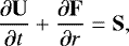 (B.6)
(B.6)
where
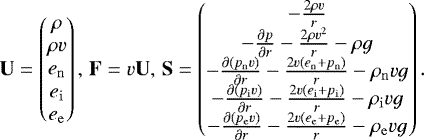 (B.7)
(B.7)
Here, U are the conserved quantities that we want to update, F are the advection fluxes of these quantities, and S are the sources. In the description below, we use the subscript j to refer to the cell index and the superscript n to refer to the timestep number, such that  is the value of U at the jth cell and the nth timestep. The subscript j + 1∕2 is used to refer to quantities at the boundary between the jth and (j + 1)th cells at radius rj+1∕2 = (rj+1 − rj)∕2.
For the time integration, we split these equations into advection and source steps using Strang splitting. This means that we first evolve U by half a timestep due to the sources, then evolve the updated values of U a full timestep due to advection, and finally evolve U again a halftimestep due to the sources5. For each one of these updates, we use the 2nd order Total Variation Diminishing (TVD) Runge–Kutte scheme given by Gottlieb & Shu (1998), given by
![Mathematical equation: \begin{eqnarray}&& \mathbf{U}^{(1)} = \mathbf{U}^{n} + {\mathrm{\Delta}} t f(\mathbf{U}^{n}) , \\ [3pt]&& \mathbf{U}^{n+1} = \frac{1}{2} \left( \mathbf{U}^{n} + \mathbf{U}^{(1)} \right) + \frac{1}{2} {\mathrm{\Delta}} t f(\mathbf{U}^{(1)}) , \end{eqnarray}](/articles/aa/full_html/2018/09/aa32776-18/aa32776-18-eq77.png)
where f(Un) is ∂U ∕∂t calculated from Un. The first step is the standard Forward Euler method, and the second step improves the approximation. When doing the two source term updates, Δ t above should be replaced with Δt∕2.
For the advection part (i.e. S = 0), Eq. (B.6) can be expressed in terms of the boundary fluxes as
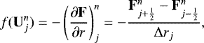 (B.10)
where Δrj = rj+1∕2 − rj−1∕2 is the cell width. To calculate the cell boundary fluxes, we use the MUSCL approach using the high-resolution TVD Lax–Friedrichs numerical flux and the minmod slope limiter (see Sects. 3.5.1 and 3.5.4 of Yee 1989). In the following discussion, we do not write the superscript n and all quantities should be assumed to be from the nth timestep. The basic idea of the MUSCL approach is instead of calculating the flux  from the adjacent cell centre values of U (i.e. Uj and Uj+1), we calculate it from left and right values of
  , given by
![Mathematical equation: \begin{eqnarray}&& \mathbf{U}_{j+\frac{1}{2}}^{\mathrm{L}} = \mathbf{U}_{j} + \frac{1}{4} \left[ \left( 1 - \eta \right) \widetilde{\widetilde{\boldsymbol{{\mathrm{\Delta}}}}}_{j-\frac{1}{2}} + \left( 1 + \eta \right) \widetilde{\boldsymbol{{\mathrm{\Delta}}}}_{j+\frac{1}{2}} \right] , \\ [3pt] && \mathbf{U}_{j+\frac{1}{2}}^{\mathrm{R}} = \mathbf{U}_{j+1} - \frac{1}{4} \left[ \left( 1 - \eta \right) \widetilde{\boldsymbol{{\mathrm{\Delta}}}}_{j+\frac{3}{2}} + \left( 1 + \eta \right) \widetilde{\widetilde{\boldsymbol{{\mathrm{\Delta}}}}}_{j+\frac{1}{2}} \right] , \end{eqnarray}](/articles/aa/full_html/2018/09/aa32776-18/aa32776-18-eq81.png)
where
![Mathematical equation: \begin{eqnarray}&& \widetilde{\boldsymbol{{\mathrm{\Delta}}}}_{j+\frac{1}{2}} = \mathrm{minmod}( \boldsymbol{{\mathrm{\Delta}}}_{j+\frac{1}{2}} , \omega \boldsymbol{{\mathrm{\Delta}}}_{j-\frac{1}{2}} ), \\ [3pt] && \widetilde{\widetilde{\boldsymbol{{\mathrm{\Delta}}}}}_{j+\frac{1}{2}} = \mathrm{minmod}( \boldsymbol{{\mathrm{\Delta}}}_{j+\frac{1}{2}} , \omega \boldsymbol{{\mathrm{\Delta}}}_{j+\frac{3}{2}} ), \end{eqnarray}](/articles/aa/full_html/2018/09/aa32776-18/aa32776-18-eq82.png)
and Δj+1∕2 = Uj+1 −Uj. The quantities η and ω are discussed below. The minmod slope limiter is given by
![Mathematical equation: \begin{equation*} \mathrm{minmod}( x , \omega y ) = \frac{|x|}{x} \max \left[ 0 , \min \left( |x| , \frac{\omega y |x|}{x} \right) \right]. \end{equation*}](/articles/aa/full_html/2018/09/aa32776-18/aa32776-18-eq83.png) (B.15)
(B.15)
In the MUSCL scheme, the TVD Lax–Friedrichs numerical flux is
![Mathematical equation: \begin{eqnarray*} \mathbf{F}_{j+\frac{1}{2}} &=& \frac{1}{2} \left[ \mathbf{F} \left( \mathbf{U}_{j+\frac{1}{2}}^{\mathrm{L}} \right) + \mathbf{F} \left( \mathbf{U}_{j+\frac{1}{2}}^{\mathrm{R}} \right) \right] \nonumber \\* & & - \frac{{\mathrm{\Delta}} t}{2 {\mathrm{\Delta}} r_{j+\frac{1}{2}}} \left( \mathbf{U}_{j+\frac{1}{2}}^{\mathrm{R}} - \mathbf{U}_{j+\frac{1}{2}}^{\mathrm{L}} \right) , \end{eqnarray*}](/articles/aa/full_html/2018/09/aa32776-18/aa32776-18-eq84.png) (B.16)
(B.16)
where  . To calculate the fluxes on the RHS of this equation, we use
![Mathematical equation: \begin{eqnarray}&& \mathbf{F} \left( \mathbf{U}_{j+\frac{1}{2}}^{\mathrm{L}} \right) = \frac{\left( \rho v \right)_{j+\frac{1}{2}}^{\mathrm{L}}}{\rho_{j+\frac{1}{2}}^{\mathrm{L}}} \mathbf{U}_{j+\frac{1}{2}}^{\mathrm{L}} , \\ [3pt]&& \mathbf{F} \left( \mathbf{U}_{j+\frac{1}{2}}^{\mathrm{R}} \right) = \frac{\left( \rho v \right)_{j+\frac{1}{2}}^{\mathrm{R}}}{\rho_{j+\frac{1}{2}}^{\mathrm{R}}} \mathbf{U}_{j+\frac{1}{2}}^{\mathrm{R}}. \end{eqnarray}](/articles/aa/full_html/2018/09/aa32776-18/aa32776-18-eq86.png)
Here,  and
and  are elements of
  and
and  and
and  are elements of
  . The value of η chosen determines the spatial order of accuracy of the scheme; we take η = 1∕3, making the scheme third-order accurate in space with an upwind bias. Given that value of η, the value of ω is an adjustable parameter with a maximum of 4; we assume ω = 3.5.
The equation for the source term updates is
 (B.19)
where S is given by Eq. (B.7). The only assumption that needs to be made to discreetise S is for the pressure source terms since they contain spatial derivatives. For these terms, we simply use central differencing.
We have performed several tests of our implementation of this algorithm, including using it to calculate the structure of a 1D isothermal stellar wind with a known analytic solution (Parker 1958). In this test, our calculations match the analytic solutions exactly. We have tested our hydrodynamics solver using the Versatile Advection Code (VAC; Tóth 1996) and find that it performs well in the standard Sod shock tube test, though VAC is less diffusive at low spatial resolution. Finally, we are able to reproduce well the hydrodynamic atmosphere simulations of Johnstone et al. (2015b), also performed using VAC.
We must also evolve the densities of individual species due to advection. To do this, we convert the cell boundary fluxes for mass into cell boundary fluxes for individual species using a simple upwind approximation for the mixing ratios of individual species at the cell boundaries. Specifically, the mixing ratios for each species are assumed to be equal to those at the centre for the cell that the mass is flowing from, meaning that if the flux is positive at the j + 1∕2 boundary, then the mixing ratio at the jth cell is taken.For the kth species, the flux is
 (B.20)
With these fluxes, we then calculate the update for the densities in each cell using a simple forward Euler method for the time integration, such that
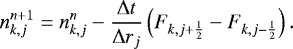 (B.21)
After this update, small inconsistencies between the values of ρ and the values of nk at each cell are corrected for by scaling the nk values such that ∑kmknk = ρ.
Appendix C Tridiagonal matrix algorithm
The tridiagonal matrix algorithm is a commonly used algorithm and detailed descriptions of the method can be found in many textbooks. Since we apply this solver for several different parts of the model, it is necessary to repeat the main steps in the algorithm here for the explanations in the following appendices to make sense. The form of the algorithm presented here is adapted from Bodenheimer et al. (2007).
The aim of the algorithm is to solve the tridiagonal systems of equations, which can be written as a system of simultaneous equations, each given by
 (C.1)
(C.1)
In our solvers, we have one of these equations for each grid cell. In the tridiagonal matrix algorithm, the coefficients aj, bj, cj, and dj are known, and the aim is to calculate xj, which represents the physical quantity of interest. The aim in the next three appendices is to derive expressions for these coefficients, and Hj and Yj discussed below, for the different physical mechanisms.
To solvethis system of equations, consider the equation
 (C.2)
(C.2)
Firstly, the values of Hj and Yj need to be calculated for each value of j except for j = J. Assuming we know HJ−1 and YJ−1 which are derived separately for each problem, the other values are calculated by iterating downwards through the grid using
 (C.3)
(C.3)
and
 (C.4)
(C.4)
With Hj and Yj known, the values of xj is calculated at each cell by iterating upwards using Eq. (C.2) and assuming that the value of x1 is known in advance (this is always the case since we use fixed lower boundary values for all quantities).
Appendix D Solver for semi-static hydrodynamic equations
We discuss in this appendix first the method used to solve the energy equations and then the method used to solve the equations for ρ and v when solving the hydrodynamics using the semi-static method presented in Sect. 2.2. It is convenient to update the energy each timestep using an implicit method since this avoids the restrictively short timestep sizes needed in the explicit schemes. The hydrodynamic part of the energy equation including gravity is
![Mathematical equation: \begin{equation*}\frac{\partial e }{ \partial t} = - \frac{1}{r^2} \frac{\partial \left[ r^2 {\mathrm{\Phi}}_e \right] }{\partial r} - \rho v g , \end{equation*}](/articles/aa/full_html/2018/09/aa32776-18/aa32776-18-eq100.png) (D.1)
(D.1)
where  . For this section, we do not write the subscripts n, i, and e for the neutral, ion, and electron components; the method presented here is used to solve the energy equations for each component separately. Using the Crank–Nicolson method for time discreetization, and the cell boundary values to discreetise cell centered spatial derivatives, we get
 (D.2)
(D.2)
This can be rewritten
![Mathematical equation: \begin{eqnarray*}e_j^{n+2} + k_j \left( r_{j+\frac{1}{2}}^2 {\mathrm{\Phi}}_{e,j+\frac{1}{2}}^{n+1} - r_{j-\frac{1}{2}}^2 {\mathrm{\Phi}}_{e,j-\frac{1}{2}}^{n+1} \right) &=& e_j^n - k_j \nonumber \\[3pt] && \times \left( r_{j+\frac{1}{2}}^2 {\mathrm{\Phi}}_{e,j+\frac{1}{2}}^{n} - r_{j-\frac{1}{2}}^2 {\mathrm{\Phi}}_{e,j-\frac{1}{2}}^{n} \right) \nonumber \\[2.5pt] && - \rho_j v_j g_j {\mathrm{\Delta}} t , \vspace*{-4pt}\end{eqnarray*}](/articles/aa/full_html/2018/09/aa32776-18/aa32776-18-eq103.png) (D.3)
(D.3)
where
 (D.4)
(D.4)
To get Φe at cell boundaries, we assume that the cell boundary values of spatially variable quantities are the average of the cell centre values; for example  . Therefore, the cell boundary fluxes is given by
![Mathematical equation: \begin{eqnarray*}{\mathrm{\Phi}}_{e,j+\frac{1}{2}}^{n} & = & \frac{1}{2} \gamma_{j+\frac{1}{2}} v_{j+\frac{1}{2}} e_j^{n} + \frac{1}{2} \gamma_{j+\frac{1}{2}} v_{j+\frac{1}{2}} e_{j+1}^{n} \nonumber \\[3pt] & & - \frac{1}{2} (\gamma_{j+\frac{1}{2}} - 1) \rho_{j+\frac{1}{2}} v_{j+\frac{1}{2}}^3. \end{eqnarray*}](/articles/aa/full_html/2018/09/aa32776-18/aa32776-18-eq106.png) (D.5)
(D.5)
where we have used  . The equations for
  ,
,  , and
, and  have the same form and can be obtained with the appropriate substitutions of the subscripts and superscripts.
After substituting the equations for the cell boundary fluxes into Eq. (D.3), the resulting equation can be expressed in the form of Eq. (C.1) with
![Mathematical equation: \begin{eqnarray}&& a_j = - \frac{1}{2} k_j \gamma_{j-\frac{1}{2}} v_{j-\frac{1}{2}} r_{j-\frac{1}{2}}^2 , \\ [3pt] && b_j = 1 + \frac{1}{2} k_j \left( \gamma_{j+\frac{1}{2}} v_{j+\frac{1}{2}} r_{j+\frac{1}{2}}^2 - \gamma_{j-\frac{1}{2}} v_{j-\frac{1}{2}} r_{j-\frac{1}{2}}^2 \right) , \\ [3pt] && c_j = \frac{1}{2} k_j \gamma_{j+\frac{1}{2}} v_{j+\frac{1}{2}} r_{j+\frac{1}{2}}^2 , \\ [3pt] && d_j = a_j e_{j-1}^n + ( 2 - b_j ) e_j^n + c_j e_{j+1}^n - \rho_j v_j g_j {\mathrm{\Delta}} t . \end{eqnarray}](/articles/aa/full_html/2018/09/aa32776-18/aa32776-18-eq111.png)
At the lower boundary, the energies are all assumed to be fixed, such that  . At the outer boundary, we apply Eq. (C.2) giving
 (D.10)
What we need are the values of HJ−1 and YJ−1 (HJ and YJ are not needed). If we assume that the outer advective energy flux, Φe,out, is known and is a constant over the timestep, such that  , then Eq. (D.3) can be written at the outer boundary as
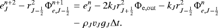 (D.11)
Inserting Eq. (D.5) for  into the above equation gives
![Mathematical equation: \begin{eqnarray}H_{J-1} \left( 1 - \frac{1}{2} k_J r_{J-\frac{1}{2}}^2 \gamma_{J-\frac{1}{2}} v_{J-\frac{1}{2}} \right) &=& \frac{1}{2} k_J r_{J-\frac{1}{2}}^2 \gamma_{J-\frac{1}{2}} v_{J-\frac{1}{2}} , \\ [3pt] \small Y_{J-1} \left( 1 - \frac{1}{2} k_J r_{J-\frac{1}{2}}^2 \gamma_{J-\frac{1}{2}} v_{J-\frac{1}{2}} \right) &=& e_J^n - 2 k_J r_{J+\frac{1}{2}}^2 {\mathrm{\Phi}}_{\mathrm{e,out}} \nonumber \\*[2pt] &-& k_J r_{J-\frac{1}{2}}^2 {\mathrm{\Phi}}_{e,J-\frac{1}{2}}^{n} - \rho_J v_J g_J {\mathrm{\Delta}} t \nonumber \\*[2pt] &-& \frac{1}{2} k_J r_{J-\frac{1}{2}}^2 \left( \gamma_{J-\frac{1}{2}} - 1 \right) \nonumber \\*[2pt] & \times & \rho_{J-\frac{1}{2}} v_{J-\frac{1}{2}}^3 . \normalsize \end{eqnarray}](/articles/aa/full_html/2018/09/aa32776-18/aa32776-18-eq117.png)
These are used to calculate HJ−1 and YJ−1. In this paper, we set Φe,out to zero.
To calculate v at all grid cells, we assume that v at the exobase is already known and integrate downwards from the exobase to the lower boundary of our simulation domain using Eq. (12). We use the Crank–Nicolson discretisation of the dv∕dr term, which gives
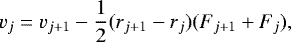 (D.14)
where 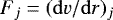 is calculated from Eq. (12). When integrating from the (j + 1)th to the jth cell, we assume dT∕dr = (Tj+1 − Tj)∕(rj+1 − rj) and make a similar assuming for
  . To get a first estimate of vj, we assume Fj = Fj+1, and the above equation becomes the Forward Euler method. We then iteratively improve this estimate using Newton iteration, given by
 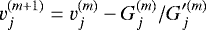 , where the superscript (m) indicates the quantity is for the mth iteration. The functions
  and
and  are given by
![Mathematical equation: \begin{eqnarray}&& G_j^{(m)} = v_j^{(m)} - v_{j+1} + \frac{1}{2} ( r_{j+1} - r_j ) ( F_{j+1} + F_j^{(m)} ), \\ [3pt] && G_j'^{(m)} = \frac{ {\rm{d}}G_j }{ {\rm{d}}v_j } = 1 + \frac{1}{2} ( r_{j+1} - r_j ) F_j'^{(m)}, \end{eqnarray}](/articles/aa/full_html/2018/09/aa32776-18/aa32776-18-eq124.png)
where  . Differentiating Eq. (12) with respect to v gives
 (D.17)
We iteratively improve our estimate of vj until  , which indicates that the solution has converged. To calculate ρ, we integrate upwards through the simulation domain using Eq. (13) and the method is essentially the same as the method for v.
Appendix E Solver for diffusion equations
In spherical coordinates, the equation for the rate of change of the density of a species at a certain point in space is
 (E.1)
(E.1)
where n is the species density and Φ is the diffusion flux given by Eqs. (23) and (24). For this section, we remove the subscript d from the flux, such that Φ = Φd. We also remove the subscript that indicates which species the quantities refer to, and apply this method to each species separately. As before, the subscript j refers to the jth radial cell and the superscript n refers to the nth timestep.
Consider the jth radial cell in the grid and assume that the subscripts j − 1∕2 and j + 1∕2 refer to the boundaries of this cell, meaning that the cell boundary diffusion fluxes are given by Φj−1∕2 and Φj+1∕2. For the spatial discreetisation, the spatial derivative in Eq. (E.1) can be written
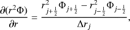 (E.2)
(E.2)
where Δrj = rj+1∕2 − rj−1∕2. For the timediscreetisation, we use the Crank–Nicolson method, such that the time derivative in Eq. (E.1) is written
![Mathematical equation: \begin{equation*}\frac{ n_{j}^{n+1} - n_{j}^n }{ {\mathrm{\Delta}} t } = \frac{1}{2} \left[ \left( \frac{\partial n}{\partial t} \right)^{n+1} + \left( \frac{\partial n}{\partial t} \right)^n \right] , \end{equation*}](/articles/aa/full_html/2018/09/aa32776-18/aa32776-18-eq130.png) (E.3)
(E.3)
where Δt = tn+1 − tn. The fact that the rate of change at the end of the update, which depends on the result of the update, is used to do the update itself is the reason that this method is implicit. These equations can be combined to give
![Mathematical equation: \begin{eqnarray*}n_{j}^{n+1} + k_j \left[ r_{j+\frac{1}{2}}^2 {\mathrm{\Phi}}_{j+\frac{1}{2}}^{n+1} - r_{j-\frac{1}{2}}^2 {\mathrm{\Phi}}_{j-\frac{1}{2}}^{n+1} \right] &=& n_{j}^n - k_j \nonumber \\*[3pt] && \times \left[ r_{j+\frac{1}{2}}^2 {\mathrm{\Phi}}_{j+\frac{1}{2}}^n - r_{j-\frac{1}{2}}^2 {\mathrm{\Phi}}_{j-\frac{1}{2}}^n \right] , \vspace*{-11pt}\end{eqnarray*}](/articles/aa/full_html/2018/09/aa32776-18/aa32776-18-eq131.png) (E.4)
(E.4)
where
 (E.5)
(E.5)
To simplify the evaluation of Eq. (E.4), the diffusion flux (Eqs. (23) and (24)) can be rewritten as
![Mathematical equation: \begin{eqnarray*}{\mathrm{\Phi}} &=& - (D + K_{\mathrm{E}}) \frac{\partial n}{\partial r} + \frac{1}{N} \frac{\partial N}{\partial r} \left( \frac{m}{\bar{m}} D + K_{\mathrm{E}} \right) n \nonumber\\[4pt] && - D \left( 1 + \alpha_{\mathrm{T}} - \frac{m}{\bar{m}} \right) \frac{1}{T} \frac{\partial T}{\partial r} n, \end{eqnarray*}](/articles/aa/full_html/2018/09/aa32776-18/aa32776-18-eq133.png) (E.6)
(E.6)
where the quantities are defined under Eq. (24). For simplicity, we assume that the cell boundary values are the averages of the cell centre values, such that 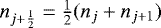 . For the derivatives, we use a simple central difference, such that
  . We make the same assumptions for all other quantities when necessary. Since the cell width is not constant, the term rj+1 − rj is different from the widths of the cells, given by Δrj. Inserting these into Eq. (E.6) and rearranging gives
![Mathematical equation: \begin{eqnarray*}{\mathrm{\Phi}}_{j+\frac{1}{2}} &= & \left[ f_{j+\frac{1}{2}} + \frac{ D_{j+\frac{1}{2}} + K_{E,j+\frac{1}{2}} }{ r_{j+1} - r_j } \right] n_{j} \nonumber \\[4pt] & & + \left[ f_{j+\frac{1}{2}} - \frac{ D_{j+\frac{1}{2}} + K_{E,j+\frac{1}{2}} }{ r_{j+1} - r_j } \right] n_{j+1} , \end{eqnarray*}](/articles/aa/full_html/2018/09/aa32776-18/aa32776-18-eq136.png) (E.7)
(E.7)
where
 (E.8)
(E.8)
The equation for the flux at the other boundary is
![Mathematical equation: \begin{eqnarray*}{\mathrm{\Phi}}_{j-\frac{1}{2}} & = & \left[ f_{j-\frac{1}{2}} + \frac{ D_{j-\frac{1}{2}} + K_{E,j-\frac{1}{2}} }{ r_j - r_{j-1} } \right] n_{j-1} \nonumber \\ & & + \left[ f_{j-\frac{1}{2}} - \frac{ D_{j-\frac{1}{2}} + K_{E,j-\frac{1}{2}} }{ r_j - r_{j-1} } \right] n_{j} , \end{eqnarray*}](/articles/aa/full_html/2018/09/aa32776-18/aa32776-18-eq138.png) (E.9)
(E.9)
where the equation for  can be obtained simply by substituting the subscripts j + 1∕2 with j − 1∕2 in Eq. (E.8).
A fundamental assumption that is made here is that all quantities except the species densities, n, in Eqs. (E.7) and (E.9) are constant over the diffusion timestep and can be calculated using the state of the simulation at the beginning of the timestep. This is not strictly true since several of the quantities, most obviously  , themselves evolve due to the changing values of n. This means that the
  term can be obtained by replacing the nj and nj+1 terms in Eq. (E.7) with
  and
and  ; similar substitutions can be madefor
  ,
,  , and
, and  .
.
Using Eqs. (E.7)–(E.9), it is possible to rewrite Eq. (E.4) in the form of Eq. (C.1), with  and the coefficients being given by
![Mathematical equation: \begin{eqnarray}a_j &=& - k_j r_{j-\frac{1}{2}}^2 \left( f_{j-\frac{1}{2}} + \frac{ D_{j-\frac{1}{2}} + K_{E,j-\frac{1}{2}} }{ r_j - r_{j-1} } \right) , \\ [3pt]b_j &=& 1 + k_j r_{j+\frac{1}{2}}^2 \left( f_{j+\frac{1}{2}} + \frac{ D_{j+\frac{1}{2}} + K_{E,j+\frac{1}{2}} }{ r_{j+1} - r_j } \right) \nonumber \\ && - k_j r_{j-\frac{1}{2}}^2 \left( f_{j-\frac{1}{2}} - \frac{ D_{j-\frac{1}{2}} + K_{E,j-\frac{1}{2}} }{ r_j - r_{j-1} } \right) , \\ [3pt]c_j &=& k_j r_{j+\frac{1}{2}}^2 \left( f_{j+\frac{1}{2}} - \frac{ D_{j+\frac{1}{2}} + K_{E,j+\frac{1}{2}} }{ r_{j+1} - r_j } \right) , \\ [3pt]d_j &=& a_j n_{j-1}^n - \left( 2 - b_j \right) n_j^n + c_j n_{j+1}^n . \end{eqnarray}](/articles/aa/full_html/2018/09/aa32776-18/aa32776-18-eq148.png)
At the lower boundary, the densities are all assumed to be fixed, such that  . At the outer boundary, the values of HJ−1 and YJ−1 are needed. Assume the outward diffusion flux at the outer boundary is known and given by Φout. Assuming also that the outward flux is a constant over the diffusion timestep, such that
 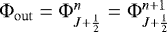 , Eq. (E.4) can be rewritten as
 (E.14)
Inserting Eq. (E.9) for  , this can be rewritten as
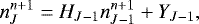 (E.15)
where
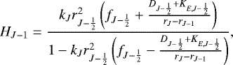 (E.16)
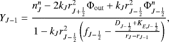 (E.17)
where  can be obtained by Eq. (E.9). If outflow conditions are desired at the upper boundary instead of imposing an outward flux, then
  and these expressions should be replaced with HJ−1 = 1 and YJ−1 = 0.
Appendix F Solver for conduction equations
In this appendix, we give the method for solving a general conduction equation with the same form as Eq. (48). This can easily be applied therefore to solving the conduction equations for the ion and electron gases; for the conduction equation for the neutral gas, which includes extra terms related to eddy conduction, the necessary modifications are given at the end of this section. Theconduction equation to solve is
 (F.1)
(F.1)
where the energy flux, Φc, is given by
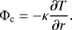 (F.2)
(F.2)
We assume here that the conductivity is a constant over the timestep, such that κ = κn = κn+1 and can be calculated using the state of the system at the beginning of the conduction timestep. This is not strictly true, since the conductivity is itself temperature dependent.
Since over the conduction timestep, e evolves only due to changes in the temperature, we can write
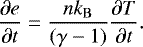 (F.3)
(F.3)
Using cell boundary values to discreetise cell centred spatial derivatives, the Crank–Nicolson discreetization of Eq. (F.1) is
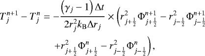 (F.4)
(F.4)
which can be rewritten as
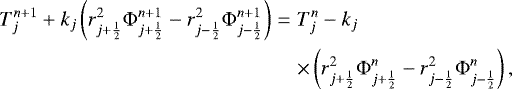 (F.5)
(F.5)
where
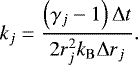 (F.6)
(F.6)
For the cell boundary fluxes, we assume
![Mathematical equation: \begin{eqnarray}&& {\mathrm{\Phi}}_{j+\frac{1}{2}}^n = - \kappa_{j+\frac{1}{2}} \frac{ T_{j+1}^n - T_{j}^n }{ r_{j+1} - r_{j} },\\ [3pt]&& {\mathrm{\Phi}}_{j-\frac{1}{2}}^n = - \kappa_{j-\frac{1}{2}} \frac{ T_{j}^n - T_{j-1}^n }{ r_{j} - r_{j-1} }, \end{eqnarray}](/articles/aa/full_html/2018/09/aa32776-18/aa32776-18-eq164.png)
where 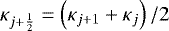 and
and  . We can combine these two relations to get
 (F.9)
(F.9)
where
 (F.10)
Similarly for Φn+1, we get
 (F.11)
By inserting Eq. (F.10) into Eq. (F.5), an equation in the form of Eq. (C.1) can be derived where  and
and
![Mathematical equation: \begin{eqnarray}&& a_j = - k_j f_{j-\frac{1}{2}} , \\[3pt]&& b_j = 1 + k_j \left( f_{j+\frac{1}{2}} + f_{j-\frac{1}{2}} \right) , \\ [3pt]&& c_j = - k_j f_{j+\frac{1}{2}} , \\ [3pt]&& e_j = a_j T_{j-1}^n - \left( 2 - b_j \right) T_j^n + c_j T_{j+1}^n . \end{eqnarray}](/articles/aa/full_html/2018/09/aa32776-18/aa32776-18-eq171.png)
For the lower boundary, we assume  . For the upper boundary, it is necessary to know HJ−1 and YJ−1. If we assume that the outward conductive energy flux, Φc,out, is known in advance, and is constant over the timestep, we can rewrite Eq. (F.5) for the final cell as
 (F.16)
By inserting Eq. (F.8) for  , we get
![Mathematical equation: \begin{eqnarray}&& H_{J-1} = \frac{k_J f_{ J - \frac{1}{2}} }{ 1 + k_J f_{J-\frac{1}{2}} } , \\ [3pt]&& Y_{J-1} = \frac{ T_J^n - 2 k_J r_{J+\frac{1}{2}}^2 {\mathrm{\Phi}}_{\mathrm{c,out}} + k_J r_{J-\frac{1}{2}}^2 {\mathrm{\Phi}}_{J-\frac{1}{2}}^{n} }{ 1 + k_J f_{J-\frac{1}{2}} }, \end{eqnarray}](/articles/aa/full_html/2018/09/aa32776-18/aa32776-18-eq175.png)
where  should be calculated using Eq. (F.8).
The conduction equation for the neutral gas is slightly more complicated than the simple conduction equation solved here due to the additional eddy conduction process. If the conductivity is taken to be the sum of the molecular and eddy conductivities, κ = κmol + κeddy, then the full neutral conduction equation is
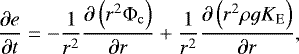 (F.19)
where ρ is the mass density, g is the gravitational acceleration, and KE is the eddy diffusion coefficient. Since the additional term on the RHS can be assumed to be constant over the conduction timestep, it only leads to additional terms in Eq. (F.15) for ej and in Eq. (sectionlinking F.18) for YJ−1. These two equations should be replaced with
![Mathematical equation: \begin{eqnarray*}e_j &= & a_j T_{j-1}^n - \left( 2 - b_j \right) T_j^n + c_j T_{j+1}^n \nonumber \\ && - \frac{\left( \gamma_j - 1 \right) {\mathrm{\Delta}} t}{2 k_{\mathrm{B}} } \left[ \rho_j \frac{K_{\mathrm{E},j+1}-K_{\mathrm{E},j-1}}{r_{j+1}-r_{j-1}} + K_{\mathrm{E},j} \frac{\rho_{j+1}-\rho_{j-1}}{r_{j+1}-r_{j-1}} \right] \end{eqnarray*}](/articles/aa/full_html/2018/09/aa32776-18/aa32776-18-eq178.png) (F.20)
(F.20)
and
![Mathematical equation: \begin{eqnarray*}Y_{J-1} &= & \frac{ T_J^n - 2 k_J r_{J+\frac{1}{2}}^2 {\mathrm{\Phi}}_{\mathrm{c,out}} + k_J r_{J-\frac{1}{2}}^2 {\mathrm{\Phi}}_{J-\frac{1}{2}}^{n} }{ 1 + k_J f_{J-\frac{1}{2}} } \nonumber \\ & & + \frac{ \frac{\left( \gamma_j - 1 \right) {\mathrm{\Delta}} t}{2 k_{\mathrm{B}} } \left[ \rho_j \frac{K_{\mathrm{E},j+1}-K_{\mathrm{E},j-1}}{r_{j+1}-r_{j-1}} + K_{\mathrm{E},j} \frac{\rho_{j+1}-\rho_{j-1}}{r_{j+1}-r_{j-1}} \right] }{ 1 + k_J f_{J-\frac{1}{2}} }. \end{eqnarray*}](/articles/aa/full_html/2018/09/aa32776-18/aa32776-18-eq179.png) (F.21)
(F.21)
The extra terms have been derived by first expanding the derivative in the final term in Eq. (F.19) using the product rule and then using central differencing on the resulting derivatives.
Appendix G Solver for energy exchange
Evolving the energies of the neutral, ion, and electron gases due to energy exchange is not completely trivial. Low in the atmosphere where the gas densities are high, the exchange rates can be large, meaning that restrictively small timesteps would be needed if an explicit integration scheme was adopted. To avoid this problem, we implement the energy exchange using the implicit Crank–Nicolson method. Unlike in the previous three appendices, we do not use the tridiagonal matrix algorithm here.
The energy exchange equations involve a large number of terms representing different forms of exchange between many different pairs of species. Most equations are not in a form that allows them to easily be solved implicitly. To simplify the problem, weassume that the exchange rates vary proportionally to the temperature differences between the components. This gives

where kei, kin, and ken are assumed to be constants. At the beginning of the energy exchange timestep, we calculate the energy exchange rates between the different components using the full sets of equations discussed in Sect. 2.5.4 and use these values, combined with the component temperatures, to calculate kei, kin, and ken.
The evolution equations for the energy densities are
The time-discreetization of these equations using the Crank–Nicolson method gives
![Mathematical equation: \begin{eqnarray}&& e_{\mathrm{n}}^{n+1} = e_{\mathrm{n}}^{n} - \frac{1}{2} {\mathrm{\Delta}} t \left( Q_{\mathrm{in}}^{n+1} + Q_{\mathrm{in}}^{n} \right) - \frac{1}{2} {\mathrm{\Delta}} t \left( Q_{\mathrm{en}}^{n+1} + Q_{\mathrm{en}}^{n} \right), \\ [3pt] && e_{\mathrm{i}}^{n+1} = e_{\mathrm{i}}^{n} - \frac{1}{2} {\mathrm{\Delta}} t \left( Q_{\mathrm{ei}}^{n+1} + Q_{\mathrm{ei}}^{n} \right) + \frac{1}{2} {\mathrm{\Delta}} t \left( Q_{\mathrm{in}}^{n+1} + Q_{\mathrm{in}}^{n} \right), \\ [3pt] && e_{\mathrm{e}}^{n+1} = e_{\mathrm{e}}^{n} + \frac{1}{2} {\mathrm{\Delta}} t \left( Q_{\mathrm{ei}}^{n+1} + Q_{\mathrm{ei}}^{n} \right) + \frac{1}{2} {\mathrm{\Delta}} t \left( Q_{\mathrm{en}}^{n+1} + Q_{\mathrm{en}}^{n} \right). \end{eqnarray}](/articles/aa/full_html/2018/09/aa32776-18/aa32776-18-eq182.png)
Since the evolution of the energy densities during the energy exchange timestep corresponds to the evolution of the temperatures, while the kinetic energy term remains constant, Eq. (F.3) can be assumed here. Inserting Eqs. (F.3) and (G.1)–(G.3) into each of these equations gives
![Mathematical equation: \begin{eqnarray}&& K_{\mathrm{en},n} T_{\mathrm{e}}^{n+1} + K_{\mathrm{in},n} T_{\mathrm{i}}^{n+1} + \left( 1 - K_{\mathrm{en},n} - K_{\mathrm{in},n} \right) T_{\mathrm{n}}^{n+1} \nonumber \\ &&= - K_{\mathrm{en},n} T_{\mathrm{e}}^{n} - K_{\mathrm{in},n} T_{\mathrm{i}}^{n} + \left( 1 + K_{\mathrm{en},n} + K_{\mathrm{in},n} \right) T_{\mathrm{n}}^{n} , \\ [3pt]&& K_{\mathrm{ei},i} T_{\mathrm{e}}^{n+1} + K_{\mathrm{in},i} T_{\mathrm{n}}^{n+1} + \left( 1 - K_{\mathrm{ei},i} - K_{\mathrm{in},i} \right) T_{\mathrm{i}}^{n+1} \nonumber \\ &&= - K_{\mathrm{ei},i} T_{\mathrm{e}}^{n} - K_{\mathrm{in},i} T_{\mathrm{n}}^{n} + \left( 1 + K_{\mathrm{ei},i} + K_{\mathrm{in},i} \right) T_{\mathrm{i}}^{n} , \\ [3pt]&& K_{\mathrm{ei},e} T_{\mathrm{i}}^{n+1} + K_{\mathrm{en},e} T_{\mathrm{n}}^{n+1} + \left( 1 - K_{\mathrm{ei},e} - K_{\mathrm{en},e} \right) T_{\mathrm{e}}^{n+1} \nonumber \\ &&= - K_{\mathrm{ei},e} T_{\mathrm{i}}^{n} - K_{\mathrm{en},e} T_{\mathrm{n}}^{n} + \left( 1 + K_{\mathrm{ei},e} + K_{\mathrm{en},e} \right) T_{\mathrm{e}}^{n} , \end{eqnarray}](/articles/aa/full_html/2018/09/aa32776-18/aa32776-18-eq183.png)
where
 (G.13)
These equations can be written in matrix form as
 (G.14)
where
![Mathematical equation: \begin{eqnarray}&& \mathbf{A} = \begin{pmatrix} A_{11} & K_{\mathrm{ei},e} & K_{\mathrm{en},e} \\ K_{\mathrm{ei},i} & A_{22} & K_{\mathrm{in},i} \\ K_{\mathrm{en},n} & K_{\mathrm{in},n} & A_{33} \end{pmatrix} , \\* [3pt]&& A_{11} = 1 - K_{\mathrm{ei},e} - K_{\mathrm{en},e} , \\* [3pt]&& A_{22} = 1 - K_{\mathrm{ei},i} - K_{\mathrm{in},i} , \\* [3pt]&& A_{33} = 1 - K_{\mathrm{en},n} - K_{\mathrm{in},n} , \\* [3pt]&& \mathbf{x} = \begin{pmatrix} T_{\mathrm{e}}^{n+1} \\ T_{\mathrm{i}}^{n+1} \\ T_{\mathrm{n}}^{n+1} \end{pmatrix} , \\* [3pt]&& \mathbf{B} = \begin{pmatrix} - K_{\mathrm{ei},e} T_{\mathrm{i}}^{n} - K_{\mathrm{en},e} T_{\mathrm{n}}^{n} + \left( 1 + K_{\mathrm{ei},e} + K_{\mathrm{en},e} \right) T_{\mathrm{e}}^{n} \\ - K_{\mathrm{ei},i} T_{\mathrm{e}}^{n} - K_{\mathrm{in},i} T_{\mathrm{n}}^{n} + \left( 1 + K_{\mathrm{ei},i} + K_{\mathrm{in},i} \right) T_{\mathrm{i}}^{n} \\ - K_{\mathrm{en},n} T_{\mathrm{e}}^{n} - K_{\mathrm{in},n} T_{\mathrm{i}}^{n} + \left( 1 + K_{\mathrm{en},n} + K_{\mathrm{in},n} \right) T_{\mathrm{n}}^{n} \end{pmatrix} . \end{eqnarray}](/articles/aa/full_html/2018/09/aa32776-18/aa32776-18-eq186.png)
At the beginning of the energy-exchange timestep, A and B are known and the aim is to calculate x, which we do using Gaussian Elimination. Once the updated temperatures are known, the updated energy densities are directly calculated.
We have tested our solver using a simpler implicit scheme based on the Backward Euler assumption and Newton iteration and find identical results. The latter scheme has the advantage that it does not require the assumptions of Eq. (G.1)–(G.3), but it is much more computationally expensive, since the exchange rates need to be calculated many times per timestep.
Appendix H Chemical network and solver
The chemical reactions in our network are listed in Table H.1. Each species varies due to chemical reactions by Eq. (22). These equations form a stiff system of ordinary differental equations (ODEs) which are impractical to solve using explicit integration methods. This is mainly because the reaction rates become very rapid in high density gases, meaning explicit integration methods require restrictively small timesteps. For example, the explicit 5th order Runge–Kutte–Fehlberg method given by Cash & Karp (1990) would require timesteps of ~ 10−7 seconds near the base of our simulations. We solve the chemical equations using an implicit multi-step Rosenbrock method. This class of methods was studied for applications to atmospheric chemistry by Sandu et al. (1997a,b), who found that they are generally more favourable than the other methods tested. The two main advantages of this method are that it is able to take large timesteps even in regions where the reaction rates are high, and that it calculates the timestep length automatically.
Assume  is the number densities of all species, where N is the number of species, and nn is this vector at time tn. The Rosenbrock method is given by
![Mathematical equation: \begin{eqnarray}&& \mathbf{n}^{n+1} = \mathbf{n}^{n} + \sum\limits_{i=1}^s b_i \mathbf{k}_i, \\ [3pt]&& \mathbf{k}_i = {\mathrm{\Delta}} t \mathbf{f}\left( \mathbf{n}^{n} + \sum\limits_{j=1}^{i-1} \alpha_{ij} \mathbf{k}_j \right) + {\mathrm{\Delta}} t \mathbf{J} \sum\limits_{j=1}^i \gamma_{ij} \mathbf{k}_j, \end{eqnarray}](/articles/aa/full_html/2018/09/aa32776-18/aa32776-18-eq188.png)
where s is the number of steps in the method, f(n) = dn∕dt (i.e. Eq. (22)) is the rate of change of n, and J = ∂f∕∂n is the Jacobian of f(n). To be clear, when i = 1, both sums in Eq. (H.2) vanish. The Jacobian is calculated analytically from Eqs. (19) and (22). Eq. (H.2) can be rearranged to give
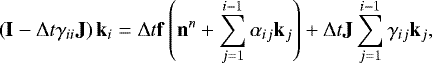 (H.3)
(H.3)
where I is the identity matrix. This is a system of linear equations of the form A ki = B, where A is an NxN matrix and B is an N element vector. We solve this system of equations to derive ki using Guassian Elimination. To perform a timestep, we calculate the values of ki sequentially and then use them to calculate nn+1.
To determine the appropriate timestep length, we first perform the update using an estimate of Δ t and then estimate the difference between our nn+1 and the exact value. Since the exact update is not known, we instead estimate this difference for the ith species as 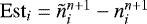 , where
  is a less accurate estimate for the update. If the method for calculating nn+1 has an order of consistency of p, then the method for calculating
  should have an order of
  . This is achieved by calculating
  using Eq. (H.2) with different values of the coefficients bi, such that
 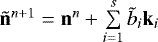 . We then estimate the error using
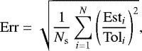 (H.4)
(H.4)
where Ns is the number of species and Toli is the error tolerance for the ith species, which we assume is given by  . As in Grassi et al. (2014), we assume aTol = 10−20 cm−3 and rTol = 10−4. We then recalculate the desired timestep length using
 (H.5)
(H.5)
If Err ≥ 1, we consider that the timestep has failed and repeat it using Δtnew as the estimatefor the Δt; otherwise, we accept our original estimate of nn+1 and use Δtnew as the estimate for Δt on the next timestep. The extra factor of 0.99 is used to reduce the need to repeat timesteps. Obviously it is often necessary to reduce Δ t when it is larger than the time that the chemistry should be evolved, especially in the upper atmosphere where chemistry timesteps ofseveral hundred seconds are possible.
The coefficients in the method are bi,  , αij, and γij. We use the coefficients derived by Sandu et al. (1997a) for their “RODAS3” method. This is a 4-step method, meaning that s = 4, and is third order, meaning that p = 3. We have tested our implementation of this solver using KROME (Grassi et al. 2014), which is a freely available package for solving chemical networks and is designed for application to atmospheric and astrophysical problems. In all tests, including full atmospheric simulations run using KROME, we find that the solvers gives almost identical results with similar computation times.
The reactions in our chemical network.
References
- Airapetian, V. S., Glocer, A., Khazanov, G. V., et al. 2017, ApJ, 836, L3 [NASA ADS] [CrossRef] [Google Scholar]
- Banks, P.M., & Kockarts, G. 1973, Aeronomy (New York: Academic Press) [Google Scholar]
- Bates, D. 1951, Proc. Physical Society. Section B, 64, 805 [NASA ADS] [CrossRef] [Google Scholar]
- Bauer, S. J., & Lammer, H. 2004, Planetary aeronomy: atmosphere environments in planetary systems (Berlin: Springer) [CrossRef] [Google Scholar]
- Bilitza, D., & Reinisch, B. W. 2008, Adv. Space Res., 42, 599 [NASA ADS] [CrossRef] [Google Scholar]
- Bodenheimer, P., Laughlin, G. P., Rózyczka, M., & Yorke, H. W. 2007, Numerical Methods in Astrophysics: An Introduction (CRC Press) [Google Scholar]
- Bougher, S. W., & Dickinson, R. E. 1988, J. Geophys. Res., 93, 7325 [NASA ADS] [CrossRef] [Google Scholar]
- Cash, J. R., & Karp, A. H. 1990, ACM Transactions on Mathematical Software (TOMS), 16, 201 [Google Scholar]
- Castle, K. J., Kleissas, K. M., Rhinehart, J. M., Hwang, E. S., & Dodd, J. A. 2006, J. Geophys. Res. (Space Phys.), 111, A09303 [NASA ADS] [CrossRef] [Google Scholar]
- Castle, K. J., Black, L. A., Simione, M. W., & Dodd, J. A. 2012, J. Geophys. Res. (Space Phys.), 117, A04310 [NASA ADS] [CrossRef] [Google Scholar]
- Chappell, C. R. 2016, Magnetosphere-Ionosphere Coupling in the Solar System No. 222 (John Wiley & Sons) [CrossRef] [Google Scholar]
- Claire, M. W., Sheets, J., Cohen, M., et al. 2012, ApJ, 757, 95 [NASA ADS] [CrossRef] [Google Scholar]
- Cohen, O., Drake, J. J., Glocer, A., et al. 2014, ApJ, 790, 57 [NASA ADS] [CrossRef] [Google Scholar]
- Curtis, A., & Goody, R. 1956, in Proc. R. Soc. Lond. Series A, Math. Phys. Sci., 236, 193 [NASA ADS] [CrossRef] [Google Scholar]
- Dickinson, R. E. 1972, J. Atm. Sci., 29, 1531 [NASA ADS] [CrossRef] [Google Scholar]
- Dickinson, R. E. 1976, Icarus, 27, 479 [NASA ADS] [CrossRef] [Google Scholar]
- Erkaev, N. V., Lammer, H., Odert, P., et al. 2013, Astrobiology, 13, 1011 [NASA ADS] [CrossRef] [Google Scholar]
- Eymet, V., Coustet, C., & Piaud, B. 2016, J. Phys.: Conf. Ser., 676, 012005 [NASA ADS] [CrossRef] [Google Scholar]
- Fontenla, J. M., Linsky, J. L., Witbrod, J., et al. 2016, ApJ, 830, 154 [NASA ADS] [CrossRef] [Google Scholar]
- Foster, J. C., St.-Maurice, J.-P., & Abreu, V. J. 1983, J. Geophys. Res., 88, 4885 [NASA ADS] [CrossRef] [Google Scholar]
- Fox, J. L. 2015, Icarus, 252, 366 [NASA ADS] [CrossRef] [Google Scholar]
- Fox, J. L., & Bougher, S. W. 1991, Space Sci. Rev., 55, 357 [NASA ADS] [CrossRef] [Google Scholar]
- Fox, J. L., & Sung, K. Y. 2001, J. Geophys. Res., 106, 21305 [NASA ADS] [CrossRef] [Google Scholar]
- Fox, J. L., Benna, M., Mahaffy, P. R., & Jakosky, B. M. 2015, Geophys. Res. Lett., 42, 8977 [NASA ADS] [CrossRef] [Google Scholar]
- García Muñoz A. 2007, Planet. Space Sci., 55, 1426 [NASA ADS] [CrossRef] [Google Scholar]
- Gilli, G., Lebonnois, S., González-Galindo, F., et al. 2017, Icarus, 281, 55 [NASA ADS] [CrossRef] [Google Scholar]
- Glocer, A., Tóth, G., Gombosi, T., & Welling, D. 2009, J. Geophys. Res. (Space Phys.), 114, A05216 [NASA ADS] [Google Scholar]
- Glocer, A., Kitamura, N., Toth, G., & Gombosi, T. 2012, J. Geophys. Res. (Space Phys.), 117, A04318 [NASA ADS] [CrossRef] [Google Scholar]
- Gottlieb, S., & Shu, C.-W. 1998, Math. Comput. Am. Math. Soc., 67, 73 [Google Scholar]
- Grassi, T., Bovino, S., Schleicher, D. R. G., et al. 2014, MNRAS, 439, 2386 [NASA ADS] [CrossRef] [MathSciNet] [Google Scholar]
- Green, A. E. S., & Barth, C. A. 1965, J. Geophys. Res., 70, 1083 [NASA ADS] [CrossRef] [Google Scholar]
- Güdel, M., Guinan, E. F., & Skinner, S. L. 1997, ApJ, 483, 947 [NASA ADS] [CrossRef] [Google Scholar]
- Hedin, A. E., Niemann, H. B., Kasprzak, W. T., & Seiff, A. 1983, J. Geophys. Res., 88, 73 [Google Scholar]
- Hoegy, W. R. 1976, Geophys. Res. Lett., 3, 541 [NASA ADS] [CrossRef] [Google Scholar]
- Hoegy, W. R. 1984, J. Geophys. Res., 89, 977 [NASA ADS] [CrossRef] [Google Scholar]
- Hollenbach, D., & McKee, C. F. 1979, ApJS, 41, 555 [NASA ADS] [CrossRef] [Google Scholar]
- Huebner, W. F., & Mukherjee, J. 2015, Planet. Space Sci., 106, 11 [Google Scholar]
- Hunten, D. M. 1974, J. Geophys. Res., 79, 2533 [NASA ADS] [CrossRef] [Google Scholar]
- Jackman, C. H., Garvey, R. H., & Green, A. E. S. 1977, J. Geophys. Res., 82, 5081 [NASA ADS] [CrossRef] [Google Scholar]
- Johnstone, C. P., & Güdel, M. 2015, A&A, 578, A129 [NASA ADS] [CrossRef] [EDP Sciences] [Google Scholar]
- Johnstone, C. P., Güdel, M., Brott, I., & Lüftinger, T. 2015a, A&A, 577, A28 [NASA ADS] [CrossRef] [EDP Sciences] [Google Scholar]
- Johnstone, C. P., Güdel, M., Stökl, A., et al. 2015b, ApJ, 815, L12 [NASA ADS] [CrossRef] [Google Scholar]
- Jusick, A., Watson, C., Peterson, L., & Green, A. 1967, J. Geophys. Res., 72, 3943 [NASA ADS] [CrossRef] [Google Scholar]
- Kasting, J. F., & Pollack, J. B. 1983, Icarus, 53, 479 [NASA ADS] [CrossRef] [Google Scholar]
- Khodachenko, M. L., Ribas, I., Lammer, H., et al. 2007, Astrobiology, 7, 167 [NASA ADS] [CrossRef] [PubMed] [Google Scholar]
- Khodachenko, M. L., Shaikhislamov, I. F., Lammer, H., & Prokopov, P. A. 2015, ApJ, 813, 50 [NASA ADS] [CrossRef] [Google Scholar]
- Kislyakova, K. G., Lammer, H., Holmström, M., et al. 2013, Astrobiology, 13, 1030 [NASA ADS] [CrossRef] [Google Scholar]
- Kislyakova, K. G., Johnstone, C. P., Odert, P., et al. 2014, A&A, 562, A116 [NASA ADS] [CrossRef] [EDP Sciences] [Google Scholar]
- Kockarts, G. 1980, Geophys. Res. Lett., 7, 137 [NASA ADS] [CrossRef] [Google Scholar]
- Körner, U., & Sonnemann, G. 2001, J. Geophys. Res.: Atmos., 106, 9639 [NASA ADS] [CrossRef] [Google Scholar]
- Kulikov, Y. N., Lammer, H., Lichtenegger, H. I. M., et al. 2007, Space Sci. Rev., 129, 207 [NASA ADS] [CrossRef] [Google Scholar]
- Kumer, J. B., & James, T. C. 1974, J. Geophys. Res., 79, 638 [NASA ADS] [CrossRef] [Google Scholar]
- Lammer, H., Lichtenegger, H. I. M., Kulikov, Y. N., et al. 2007, Astrobiology, 7, 185 [NASA ADS] [CrossRef] [PubMed] [Google Scholar]
- Lammer, H., Kasting, J. F., Chassefière, E., et al. 2008, Space Sci. Rev., 139, 399 [NASA ADS] [CrossRef] [Google Scholar]
- Lammer, H., Stökl, A., Erkaev, N. V., et al. 2014, MNRAS, 439, 3225 [NASA ADS] [CrossRef] [Google Scholar]
- Lichtenegger, H. I. M., Lammer, H., Grießmeier, J.-M., et al. 2010, Icarus, 210, 1 [NASA ADS] [CrossRef] [Google Scholar]
- Lichtenegger, H. I. M., Kislyakova, K. G., Odert, P., et al. 2016, J. Geophys. Res. (Space Phys.), 121, 4718 [Google Scholar]
- López-Morales, M., Haywood, R. D., Coughlin, J. L., et al. 2016, AJ, 152, 204 [NASA ADS] [CrossRef] [Google Scholar]
- Luger, R., Barnes, R., Lopez, E., et al. 2015, Astrobiology, 15, 57 [NASA ADS] [CrossRef] [Google Scholar]
- Marty, B., & Dauphas, N. 2003, Earth Planet. Sci. Lett., 206, 397 [NASA ADS] [CrossRef] [Google Scholar]
- Noack, L., Godolt, M., von Paris, P., et al. 2014, Planet. Space Sci., 98, 14 [NASA ADS] [CrossRef] [Google Scholar]
- Oberheide, J., Mlynczak, M. G., Mosso, C. N., et al. 2013, J. Geophys. Res. (Space Phys.), 118, 7283 [NASA ADS] [CrossRef] [Google Scholar]
- Owen, J. E., & Mohanty, S. 2016, MNRAS, 459, 4088 [NASA ADS] [CrossRef] [Google Scholar]
- Parker, E. N. 1958, ApJ, 128, 664 [Google Scholar]
- Picone, J. M., Hedin, A. E., Drob, D. P., & Aikin, A. C. 2002, J. Geophys. Res. (Space Phys.), 107, 1468 [Google Scholar]
- Ribas, I., Guinan, E. F., Güdel, M., & Audard, M. 2005, ApJ, 622, 680 [NASA ADS] [CrossRef] [Google Scholar]
- Richards, P. G., & Voglozin, D. 2011, J. Geophys. Res. (Space Phys.), 116, A08307 [Google Scholar]
- Ridley, A., Deng, Y., & Toth, G. 2006, J. Atm. Sol.-Terr. Phys., 68, 839 [NASA ADS] [CrossRef] [Google Scholar]
- Rimmer, P. B., & Helling, C. 2016, ApJS, 224, 9 [NASA ADS] [CrossRef] [Google Scholar]
- Roble, R. G. 1995, Geophysical Monograph Series, 87, 1 [Google Scholar]
- Roble, R. G., Ridley, E. C., & Dickinson, R. E. 1987, J. Geophys. Res., 92, 8745 [NASA ADS] [CrossRef] [Google Scholar]
- Rothman, L. S., Gordon, I. E., Barbe, A., et al. 2009, J. Quant. Spectr. Rad. Transf., 110, 533 [NASA ADS] [CrossRef] [Google Scholar]
- Rothman, L., Gordon, I., Barber, R., et al. 2010, J. Quant. Spectr. Rad. Transf., 111, 2139 [NASA ADS] [CrossRef] [Google Scholar]
- Sandu, A., Verwer, J., Blom, J., et al. 1997a, Atm. Environ., 31, 3459 [Google Scholar]
- Sandu, A., Verwer, J., Van Loon, M., et al. 1997b, Atm. Environ., 31, 3151 [CrossRef] [Google Scholar]
- Schunk, R. W. 1975, Planet. Space Sci., 23, 437 [NASA ADS] [CrossRef] [Google Scholar]
- Schunk, R. W., & Nagy, A. F. 1978, Rev. Geophys. Space Phys., 16, 355 [NASA ADS] [CrossRef] [Google Scholar]
- Schunk, R., & Nagy, A. 2000, Space Sci. Ser., 59, 554 [Google Scholar]
- Shaikhislamov, I. F., Khodachenko, M. L., Sasunov, Y. L., et al. 2014, ApJ, 795, 132 [NASA ADS] [CrossRef] [Google Scholar]
- Siddles, R. M., Wilson, G. J., & Simpson, C. J. S. M. 1994, J. Chem. Phys., 189, 779 [NASA ADS] [Google Scholar]
- Singhal, R. P., & Haider, S. A. 1984, J. Geophys. Res., 89, 6847 [NASA ADS] [CrossRef] [Google Scholar]
- Smithtro, C. G., & Sojka, J. J. 2005, J. Geophys. Res. (Space Phys.), 110, A08305 [NASA ADS] [Google Scholar]
- Smithtro, C. G., & Solomon, S. C. 2008, J. Geophys. Res. (Space Phys.), 113, A08307 [NASA ADS] [CrossRef] [Google Scholar]
- Swartz, W. E., Nisbet, J. S., & Green, A. E. 1971, J. Geophys. Res., 76, 8425 [NASA ADS] [CrossRef] [Google Scholar]
- Taylor, R. L., & Bitterman, S. 1969, Rev. Mod. Phys., 41, 26 [NASA ADS] [CrossRef] [Google Scholar]
- Telleschi, A., Güdel, M., Briggs, K., et al. 2005, ApJ, 622, 653 [NASA ADS] [CrossRef] [Google Scholar]
- Tian, F. 2009, ApJ, 703, 905 [NASA ADS] [CrossRef] [Google Scholar]
- Tian, F., Kasting, J. F., Liu, H.-L., & Roble, R. G. 2008a, J. Geophys. Res. (Planets), 113, E05008 [NASA ADS] [CrossRef] [Google Scholar]
- Tian, F., Solomon, S. C., Qian, L., Lei, J., & Roble, R. G. 2008b, J. Geophys. Res. (Planets), 113, E07005 [NASA ADS] [Google Scholar]
- Tóth, G. 1996, Astrophys. Lett. Commun., 34, 245 [NASA ADS] [Google Scholar]
- Tu, L., Johnstone, C. P., Güdel, M., & Lammer, H. 2015, A&A, 577, L3 [NASA ADS] [CrossRef] [EDP Sciences] [Google Scholar]
- Venot, O., Bénilan, Y., Fray, N., et al. 2018, A&A, 609, A34 [NASA ADS] [CrossRef] [EDP Sciences] [Google Scholar]
- Verronen, P. T., Turunen, E., Ulich, T., & Kyrölä, E. 2002, Annales Geophysicae, 20, 1967 [NASA ADS] [CrossRef] [Google Scholar]
- Verronen, P. T., SeppäLä, A., Clilverd, M. A., et al. 2005, J. Geophys. Res. (Space Phys.), 110, A09S32 [CrossRef] [Google Scholar]
- von Zahn, U., Fricke, K., Hunten, D., et al. 1980, J. Geophys. Res.: Space Phys., 85, 7829 [NASA ADS] [CrossRef] [Google Scholar]
- Wakelam, V., Herbst, E., Loison, J.-C., et al. 2012, ApJS, 199, 21 [NASA ADS] [CrossRef] [Google Scholar]
- Watson, C. E., Dulock, Jr. V. A., Stolarski, R. S., & Green, A. E. S. 1967, J. Geophys. Res., 72, 3961 [NASA ADS] [CrossRef] [Google Scholar]
- West, A. A., Hawley, S. L., Bochanski, J. J., et al. 2008, AJ, 135, 785 [NASA ADS] [CrossRef] [Google Scholar]
- Wintersteiner, P. P., Picard, R. H., Sharma, R. D., Winick, J. R., & Joseph, R. A. 1992, J. Geophys. Res., 97, 18 [CrossRef] [Google Scholar]
- Yee, H. C. 1989, in Computational Fluid Dynamics, 04 [Google Scholar]
- Yelle, R. V. 2004, Icarus, 170, 167 [NASA ADS] [CrossRef] [Google Scholar]
- Zahnle, K., Schaefer, L., & Fegley, B. 2010, Cold Spring Harbor perspectives in biology, 2, a004895 [Google Scholar]
Several meanings of the abbreviation “XUV” are used in the literature. In this paper, we use the term to refer to the X-ray and UV spectrum from 10 to 4000 Å.
We will make The Kompot Code publicly available in the near future, and it will be obtainable by contacting the authors directly.
To get γ for a gas mixture, we first calculate CV,j and CP,j for each species using Mayer’s relation and their individual γj values, where the subscript j refers to an individual species. Then, we calculate the total heat capacities as the density weighted average heat capacities of the constituent gases. Finally, γ is calculated simply as the ratio CP∕CV.
For example, to calculate the total XUV heating rate, we calculate 4π ∫ r2Qxuvdr, where the integral is over all radii, r, and Qxuv is the volumetric heating rate given by Eq. (26).
This can be written Un+1 = LS,Δt∕2LA,ΔtLS,Δt∕2Un, where LA and LS are the operators for updating U by advection and sources respectively. Similarly, the simpler first-order accurate Gudonov type splitting is written Un+1 = LS,ΔtLA,ΔtUn.
All Tables
All Figures
|
Fig. 1 Cartoon illustrating the geometry of the radiation transfer in our model. The bottom right of the cartoon is the centre of the planet and the incoming stellar radiation is travelling horizontally from left to right. The inner black region is the planet and the shaded region is the upper atmosphere. The simulation domain of our 1D atmosphere model, illustrated with the blue region, is a region that is pointing radially outwards from the planet centre. The angle θ is the zenithangle. To calculate the stellar XUV and IR spectra at any given point, we perform radiation transfer along the dashed black line. |
| In the text | |
|
Fig. 2 Stellar XUV irradiance spectrum at different altitudes in the atmosphere of the Earth, calculated using our current Earth model presented in Sect. 3.1. The black and purple lines show the spectrum at the top and bottom of our model respectively. |
| In the text | |
|
Fig. 3 Infrared absorption spectra of CO2 (upper panel) and H2O (lower panel) as calculated by kspectrum (Eymet et al. 2016). The gas is assumed to have a temperature of 200 K and a pressure of 10−2 mbar. The horizontal dashed line shows the cross-section of 10−22 cm−3. |
| In the text | |
|
Fig. 4 Our prediction for the non-thermal electron spectrum at 200 km for the current Earth. For comparison, the dashed lines show the spectra at several altitudes calculated by Singhal & Haider (1984; taken from their Fig. 3 and multiplied by 4πto move the sr−1 from the units). The sudden increase in the flux at low electron energies is due to the thermal electron spectrum becoming dominant. |
| In the text | |
|
Fig. 5 Simplified cartoon illustrating the main pathways taken in our model by the energy that is removed from the XUV field by absorption due to photodissociation and photoionization reactions. In both cases, much of the energy used to cause the photoreaction is released due to exothermic chemical reactions. For photodissociation, the remaining energy from the absorbed photon is given to the thermal energy budget of the neutral gas directly. For photoionization, the remaining energy is released as kinetic energy of the produced electron, and is then lost as the electron collides with the ambient gas; collisions with neutral species are inelastic and lead to excitation, dissociation, and ionization, whereas collisions with ambient thermal electrons are elastic and lead to heating of the electron gas. |
| In the text | |
|
Fig. 6 Escape probability of a 15 μm photon as a function of CO2 optical depth (upper panel) and the CO2 deexcitation rate coefficients as a function of temperature (lower panel). In the upper panel, the numbers show the approximate altitudes in our current Earth model where these points on the line are reached. In the lower panel, the data points are measurements from Siddles et al. (1994) and Castle et al. (2012), and the solid lines are our power-law fits, given in Table 1. |
| In the text | |
|
Fig. 7 Neutral, ion, and electron temperature structures of our current Earth model. The dashed black line is for the empirical NRLMSISE-00 model. |
| In the text | |
|
Fig. 8 Thermal processes in our Earth model as functions of altitude. In the upper panel, the red line shows the total XUV, chemical, and Joule heating, the blue line shows the total IR cooling, the cyan and magenta lines show the neutral heating by collisions with electron and ions, the black line shows the sum of all of these, and the green line shows the effects conduction. In the middle and lower panels, we show the contributions of individual mechanisms to the total heating and cooling. |
| In the text | |
|
Fig. 9 Density structures of several important neutral (upper panel) and ion (lower panel) species. The solid lines show the predictions of our model and the dotted lines are from the empirical NRLMSISE-00 model for the neutrals and the IRI-2007 model for the ions. |
| In the text | |
|
Fig. 10 Results of our modern Venus model. In the upper left panel, showing the temperature profiles, the dashed black line shows the empirical model by Hedin et al. (1983) and the dotted black line shows the daytime profiles shown in Fig. 9 of Gilli et al. (2017). In the upper right panel, showing the density profiles of several important species, the solid lines show the results of our model and the dotted lines show the profiles given by Hedin et al. (1983). The lower left panel shows the heating and cooling mechanisms for the neutral gas, and the lower right panel shows all of the heating mechanisms. |
| In the text | |
|
Fig. 11 Neutral temperature structures for our simulations with different base mixing ratios of CO2 (upper-panel) and the total atmospheric heating rates due to the various heating processes as a function of CO2 mixing ratio (lower-panel). In the upper panel, the lines (which stop at the exobase) are simulations where the base CO2 density is 0.01, 0.1, 1, 10, 100, and 1000 times the value for the current Earth, which has a mixing ratio at 65 km of 4 × 10⁻⁴. |
| In the text | |
|
Fig. 12 Temperatures (upper panel), altitudes (middle panel), and mixing ratios of several important species of the exobase (lower panel) as a function of the CO2 mixing ratio at 65 km. In the lower panel, the black line gives the total ion mixing ratio (i.e. the ionization fraction). |
| In the text | |
|
Fig. 13 Our simulation results for the response of the Earth’s atmosphere to the evolving XUV spectrum of the Sun. In the upper left panel, we show the temperature structures for several of these models, where the different colours are for different ages and the solid, dashed, and dotted lines show the neutral, ion, and electron temperatures respectively. In all cases, the lines end at the exobase. In the upper right, middle left, and middle right panels, we show the exobase temperatures, altitudes, and chemical compositions as functions of age. In the lower left and lower right panels, we show the evolution of Jeans escape for H, O, N, and He, with the difference between the two plots being the range on the y-axis. In each figure, the small circles show the exact locations of each simulation. |
| In the text | |
|
Fig. 14 Evolution of direct XUV heating (upper panel), chemical heating (middle panel), and photoelectron heating (lower panel) within three altitude ranges in the Earth’s atmosphere. The quantities plotted are the total heating rates integrated over the relevant volumes and normalised to the values for the modern Earth. For photoelectron heating, only the values for altitudesbetween 200 km and the exobase are shown since at lower altitudes this process is negligible. |
| In the text | |
Current usage metrics show cumulative count of Article Views (full-text article views including HTML views, PDF and ePub downloads, according to the available data) and Abstracts Views on Vision4Press platform.
Data correspond to usage on the plateform after 2015. The current usage metrics is available 48-96 hours after online publication and is updated daily on week days.
Initial download of the metrics may take a while.