| Issue |
A&A
Volume 616, August 2018
|
|
|---|---|---|
| Article Number | L8 | |
| Number of page(s) | 5 | |
| Section | Letters to the Editor | |
| DOI | https://doi.org/10.1051/0004-6361/201833156 | |
| Published online | 20 August 2018 | |
Letters to the Editor
Simulating the pericentre passage of the Galactic centre star S2
1
Universitäts-Sternwarte München, Scheinerstraße 1, 81679 München, Germany
e-mail: This email address is being protected from spambots. You need JavaScript enabled to view it.
2
Max-Planck-Institut für extraterrestrische Physik, Postfach 1312, Giessenbachstr. 1, 85741 Garching, Germany
3
INAF – Osservatorio Astronomico di Padova, Vicolo dell’Osservatorio 5, 35122 Padova, Italy
Received:
4
April
2018
Accepted:
30
July
2018
Abstract
Context. Our knowledge of the density distribution of the accretion flow around Sgr A* – the massive black hole (BH) at our Galactic centre (GC) – relies on two measurements only: one at a distance of a few Schwarzschild radii (Rs) and one at roughly 105 Rs, which are usually bridged by a power law, which is backed by magnetohydrodynamical simulations. The so-called S2 star reached its closest approach to the massive BH at around 1500 Rs in May 2018. It has been proposed that the interaction of its stellar wind with the high-density accretion flow at this distance from Sgr A* will lead to a detectable, month-long X-ray flare.
Aims. Our goal is to verify whether or not the S2 star wind can be used as a diagnostic tool to infer the properties of the accretion flow towards Sgr A* at its pericentre (an unprobed distance regime), putting important constraints on BH accretion flow models. Methods. We run a series of three-dimensional adaptive mesh refinement simulations with the help of the RAMSES code which include the realistic treatment of the interaction of S2’s stellar wind with the accretion flow along its orbit and – apart from hydrodynamical and thermodynamical effects – include the tidal interaction with the massive BH. These are post-processed to derive the X-ray emission in the observable 2–10 keV window.
Results. No significant excess of X-ray emission from Sgr A* is found for typical accretion flow models. A measurable excess is produced for a significantly increased density of the accretion flow. This can, however, be ruled out for standard power-law accretion flow models as in this case the thermal X-ray emission without the S2 wind interaction would already exceed the observed quiescent luminosity. Only a significant change of the wind parameters (increased mass loss rate and decreased wind velocity) might lead to an (marginally) observable X-ray flaring event.
Conclusion. Even the detection of an (month-long) X-ray flare during the pericentre passage of the S2 star would not allow for strict constraints to be put on the accretion flow around Sgr A* due to the degeneracy caused by the dependence on multiple parameters (of the accretion flow model as well as the stellar wind).
Key words: Galaxy: center / stars: winds, outflows / hydrodynamics / accretion, accretion disks / black hole physics / gravitation
© ESO 2018
1. Introduction
The massive central black hole (BH) makes the Galactic centre (GC) a unique laboratory to study gas and stellar dynamics in an extreme environment. With a visual extinction of AV ≈ 30 mag (Becklin & Neugebauer 1968; Rieke et al. 1989), corresponding to a column density of 1.6 × 1023 cm−2(Ponti et al. 2017), the obscuring medium becomes partially transparent to X-rays with energies above 2 keV. In the spectral window between 2 and 10 keV, Baganoff et al. (2003) found a source with a full width at half maximum (FWHM) of 1.4 as (≈0.06 pc) and an absorption corrected luminosity of 2.4 × 1033 erg s−1 (with roughly a factor of two uncertainty) at the position of Sgr A*, the compact nonthermal radio source (Balick & Brown 1974; Backer 1996) associated with the massive BH at the dynamical centre of the Galaxy. Assuming that this emission mainly arises from thermal X-rays emitted by a hot accretion flow towards Sgr A*, Baganoff et al. (2003) fit an absorbed optically thin thermal plasma model, finding that the average electron density inside this region is ne ≈ 130 cm−3 with a temperature of kBTe ≈ 2 keV. The fuel for the accretion flow at the Bondi radius is thought to be provided by winds of a cluster of young, luminous stars (Krabbe et al. 1995; Najarro et al. 1997; Coker & Melia 1997; Quataert et al. 1999; Paumard et al. 2001). Radio observations, by measuring the polarization (from Faraday rotation) and the size of the emission, allow for the density to be roughly constrained at a distance of a few Rs (Quataert & Gruzinov 2000a; Bower et al. 2003; Marrone et al. 2007; Doeleman et al. 2008). In the region in between, the density and temperature distributions of the accretion flow are simply estimated with the help of power-law models (Sect. 2.1), backed by magnetohydrody-namical simulations. An attempt to constrain the density distribution close to the pericentre position of the G2 cloud (about 1500 Rs) was made by Plewa et al. (2017). By means of fitting test-particle simulations to the observations, they find an electron number density of around 103 cm−3. Within the same distance regime, the S-star cluster is located (Schödel et al. 2003; Ghez et al. 2005; Eisenhauer et al. 2005; Gillessen et al. 2009b). Its best observed member is the S2 star (e.g. Gillessen et al. 2009a), which is on a ~ 16 year orbit and reached its pericentre passage (also at around 1500 Rs distance) in May 2018. It is an early B-dwarf of spectral type B0-B2.5 V with a stellar wind with an estimated velocity vw ~ 1000 km s−1 and a mass-loss rate of Ṁw ≲ 3 × 10⁻⁷M⊙ yr−1 (Martins et al. 2008). It has been suggested to use the X-ray emission from the interaction of S2’s stellar wind with the accretion flow during pericentre passage to put constraints on its density structure in this so-far unprobed distance regime (Giannios & Sironi 2013; Christie et al. 2016). With the help of analytical estimates of the bow shock interaction with an already present gas distribution around Sgr A*, Giannios & Sironi (2013) estimated the X-ray emission to be significant around pericentre passage and to be sensitive to the exponent of the assumed radial (power law) profile of the accretion flow. An additional contribution to the X-ray emission during S2’s pericentre passage (which we neglect in this letter) could arise from Compton-upscattered optical/UV photons emitted from the star as was suggested by Nayakshin (2005). The radio emission has been analytically estimated by Crumley & Kumar (2013), Zajaček et al. (2016) and Ginsburg et al. (2016). Two-dimensional (2D) numerical hydrosimulations were presented by Christie et al. (2016) to estimate the increase in thermal X-ray emission during the pericentre passage of the S2 star. For their choice of parameters they find that S2’s pericentre passage leads to a detectable roughly one month long X-ray flare emission (Sect. 3.5). However, given the complex interplay of the hydrodynamical, thermodynamical, and gravitational interaction of the stellar wind shells with the ambient medium, neither the analytical estimates nor the 2D simulations are expected to capture the full complexity of the problem. Three-dimensional (3D) simulations including the evolution along the orbit are necessary and are presented in this letter. We describe the simulation setup and analysis in Sect. 2, discuss the results in Sect. 3, and conclude in Sect. 4.
2. Simulation setup and analysis
We adopt the orbital elements of the S2 star from Table 3 of Gillessen et al. (2017) with the solar distance to Sgr A* of 8.13 kpc and a mass of the central BH of 4.1 × 10⁶M⊙. We start the mechanically implemented wind (vw = 1000 km s−1 and Ṁw = 3×10⁻⁷M⊙ yr−1 for the standard simulation) in apo centre and follow its hydrodynamical, thermodynamical (adiabatic with solar metallicity cooling), and gravitational interaction using the adaptive mesh refinement code RAMSES (Teyssier 2002).
2.1. The accretion flow around Sgr A*
The quiescent galactic nucleus of the Milky Way is found to be underluminous for its estimated accretion rate with respect to standard thin accretion disc models (Baganoff et al. 2003). In order to account for this misbalance, radiatively inefficient, optically thin, geometrically thick accretion flow models have been proposed, featuring high gas temperatures and low densities that are often described by power-law radial profiles and that give rise to thermal Bremsstrahlung emission. Various exponents for the radial power-law density distribution have been suggested within the range of β = −1.5 and −0.5: the Bondi solution is described by roughly −1.5 and so-called convection-dominated accretion flow (CDAF) models (Quataert & Gruzinov 2000b) predict −0.5. A value of −1.0 has been found in simulations (e.g. McKinney et al. 2012; Narayan et al. 2012) and by analytical, so-called radiatively inefficient accretion flow (RIAF) solutions (Yuan et al. 2003). The latter has been widely used to describe the interaction of the G2 cloud with the accretion flow (Gillessen et al. 2012; Burkert et al. 2012; Schartmann et al. 2015; Ballone et al. 2013). We therefore chose this solution for our standard model, employing the same resetting technique as in Schartmann et al. (2015), due to its instability to convection. Additionally, we test other exponents of the power law density distribution, as the most recent Chandra observations favor a less steep profile with an exponent close to −0.5 (Wang et al. 2013; Roberts et al. 2017). We normalise the accretion flow models so as to obtain the observed quiescent 2–10 keV thermal emission within a radius of 0.7″ – the intrinsic size of the Sgr A* emission found by Baganoff et al. (2003). For our standard model, this results in a density distribution of (1)
(1)
where r is the distance to Sgr A*. Despite neglecting magnetic fields and rotation and setting it up in hydrostatic equilibrium, we refer to it as the “accretion flow” in the following. The simulations range from an inner radius of rin = 1.4 × 10⁻⁴ pc to the edge of a cubic box with width of roughly 3.3×10⁻² pc, reaching a minimum cell size of 4 μ pc.
2.2. Modelling the X-ray emission
The intrinsic thermal X-ray emission properties of the hot gas are calculated using the Astrophysical Plasma Emission Code (APEC) model (Smith et al. 2001) within the AtomDB (Foster et al. 2012) version 3.0.9. An optically thin, thermal plasma in collisional ionisation equilibrium (CIE) is assumed. The resulting X-ray emission per cell is then projected onto the orbital plane and images and light curves in the 2–10 keV window are calculated. We subtract the X-ray emission of our initial condition from the one obtained in the individual time steps in order to single out the excess emission due to the interaction of the stellar wind with the accretion flow.
3. Results and discussion
3.1. The wind / accretion flow interaction
Snapshots of the density evolution of our standard model are shown in Fig. 1a–d. We start the simulation itself and the stellar wind at the apocentre. As the stellar velocity is relatively small ( ) at this position, the stellar wind has time to expand and reach its stagnation radius, where the ram pressure of the wind is balanced by the thermal pressure of the ambient medium. This expansion phase excites Rayleigh–Taylor instabilities that break up the contact discontinuity and start to transform the shocked wind shell into a structure with filaments and mushroom-shaped fingers pointing outwards, but leaving the inner shock as a sharp transition towards the free streaming wind (Fig. 1a). Due to the very high pressure in the GC, the outer shock is very weak. Moving into the higher-density (and pressure) inner regions of the BH accretion flow, the free wind region decreases again and its spherical shape is turned into a drop-like shape, as the ram pressure due to the motion of the star becomes important and adds to the ambient thermal pressure in the aforementioned equilibrium. The latter causes the asymmetric location of the star in the free-wind region (Fig. 1a). Reaching very close to the BH, the evolution is dominated by tidal forces, which lead to a stretching of the build-up cloud in the radial direction and a compression perpendicular to its motion. Here we define the cloud as the gas atmosphere that accumulates around S2 due to its wind and the interaction with the surrounding gas. At this time, Rayleigh–Taylor instabilities and Kelvin–Helmholtz instabilities have already transformed the shocked-wind region into a filamentary shell (Fig. 1b), which is prone to stripping due to the ram pressure exerted by the accretion flow on the now fast-moving star (
 at pericentre distance). A small fraction of these filaments move ahead of the star and have lost enough angular momentum to the accretion flow to end up inside our inner radius (Fig. 2d), before the nominal pericentre is reached. During pericentre passage, the typical tidal disruption fan shows up and the gas that remains bound to the BH smoothes out on a short timescale caused by the very high sound speed in this region (
 ) and correspondingly short sound crossing time (
 compared to
  and
and  at apo centre). A large fraction of the shell is stripped, but already roughly 0.5 yr after pericentre a new shocked wind shell becomes visible. Moving further out in the potential, the radius of this shell around S2 increases fast (Fig. 1c). Due to the strong hydro instabilities, it forms a thick, filamentary and partly asymmetric cocoon. Its evolution is similar to the beginning of the simulation, but ram pressure interaction of the filamentary shocked wind shell with the accretion flow leads to the formation of a nozzle of gas (Fig. 1d) pointing from the upstream part of the cloud towards the BH and allows to funnel low angular momentum gas towards the direct surroundings of the minimum of the potential well and through our inner radius (see discussion in Sect. 3.2). A similar pattern as the one discussed previously starts after having reached apocentre passage.
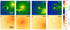 |
Fig. 1. Time evolution (given relative to the epoch of pericentre passage) of the standard model. Shown are cuts through the density distribution (centred on S2) within the orbital plane (panels a–d) and X-ray 2–10 keV emission maps (perpendicular to the orbital plane), including the emission of the accretion flow (panels e–h). The white cross depicts the location of the BH and is located outside (to the lower right) of the shown region in panels d and h. |
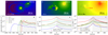 |
Fig. 2. Time evolution for a parameter study of various power-law exponents (β) and normalisations (ρ0) of the assumed accretion flow density distribution (see legend and Eq. 1), as well as stellar wind velocities vw. Shown are cuts through the density in the orbital plane at a time of 530 days before pericentre (panels a–c, same colour scale as in Fig. 1a–d; the white cross refers to the position of the BH), the mass transfer rate through the inner boundary (panel d), the variation of the electron number density of the accretion flow along the orbital path of S2 (panel e), and the light curves of excess X-ray emission (panel f). Time is given relative to the epoch of pericentre passage. The dotted magenta lines denote the accuracy of roughly a factor of two of the Baganoff et al. (2003) measurement. |
3.2. Mass transfer towards the centre
The accretion rate (of wind material only, selected by a passive tracer field) through the inner radius rin = 1.4 × 10⁻⁴ pc found in the simulation is shown in Fig. 2d (black line); it peaks close to pericentre with approximately 2 × 10⁻⁶ M⊙ yr−1, roughly corresponding to the upper limit derived from observations at this distance regime (Genzel et al. 2010). Roughly 1.5 yr after the violent pericentre passage, the accretion rate reaches an almost constant level of around 4×10⁻⁷ M⊙ yr−1, as a disc forms around the BH, which is fed by the stream of gas towards Sgr A*. The latter is first provided by gas in the dispersed tail of the source and later by the nozzle (see Sect. 3.1 and Fig. 1) of low-angular-momentum gas connecting BH and source. Therefore no drastic change in the accretion flow or its electromagnetic emission is expected to occur.
3.3. X-ray emission
Using the recipe described in Sect. 2.2, the expected thermal X-ray emission has been calculated. Being shocked by the interaction with the ambient medium, the stellar wind material heats up to temperatures of around 107 K. This gives rise to enhanced thermal X-ray emission in the 2-10 keV window compared to our background density structure (Fig. 1e–h), which roughly follows the morphology of the projected density distribution, but without showing the free-wind region around the star due to its low temperature of Tfw = 104 K. An increase of the X-ray emission is recognisable the closer the source moves towards the BH. This is caused by (i) the star accelerating into the denser part of the accretion flow (Fig. 2e, black line), (ii) the continuously increasing amount of gas in the shocked wind shell and (iii) the tidal interaction. These effects cause stronger shock heating as well as a stronger compression of the upstream part of the shocked wind shell, leading to higher densities, temperatures, and emissivity. In order to derive the corresponding light curve (black line in Fig. 2f), we subtract the X-ray emission of the accretion flow (our initial condition) and compare to the observed quiescent emission (Baganoff et al. 2003) (dashed magenta line). We find that the peak of the X-ray emission lags behind the peak of the density evolution (Fig. 2e, black line) along the orbit. This was already found by Christie et al. (2016) and was explained to be caused by the compression of the dispersed tail, which reaches the point of maximum environment density slightly later than the star itself. The light curve (Fig. 2f) is asymmetric with respect to the pericentre passage, showing a steeper gradient before pericentre compared to the evolution after pericentre. In the time frame shown, this is caused by the stream of gas falling back and interacting with the central density concentration and the mixing with high-temperature gas from the accretion flow. For our standard model, the peak (excess) X-ray emission remains significantly below the observed value (during quiescent phases of Sgr A*) and no X-ray flare event is expected.
3.4. The effect of parameter variations
In order to determine whether the S2 pericentre passage can be used to constrain the density distribution of the accretion flow, we performed an extensive parameter study. To test the influence of the ambient density on the stellar wind evolution along the orbit, we decreased and increased the normalisation of the mean density of the atmosphere by a factor of ten, in order to bracket the density inferred in Plewa et al. (2017) and the assumptions made in the simulations of Christie et al. (2016); see Fig. 2e. Keeping the temperature distribution constant, this changes the pressure distribution by the same factor and therefore has a strong influence on the stagnation radius and also on the evolution, as can be seen in Fig. 2a–c. Being able to grow to a larger size in the low-density case (Fig. 2a), the wind-blown bubble reaches the pericentre earlier and leads to an increased mass transfer rate through our inner boundary before the nominal pericentre passage time (Fig. 2d). In contrast, in the high-density ambient medium case (Fig. 2c), the mass transfer increases shortly after pericentre (Fig. 2d), but remains at a similar level to that in our standard model. In regards to the X-ray emission, the shapes of the light curves behave similarly, whereas the scaling shows the expected strong differences. The high-density ambient medium case would seemingly leave an observable X-ray footprint. However, the thermal X-ray emission from the accretion flow itself would now also exceed the observed quiescent emission, ruling out this density normalisation.
We change the power-law exponents to −0.5 and −1.5 and normalise the density distributions such that the thermal X-ray emission within 0.7″ is given by the quiescent value of Baganoff et al. (2003). This results in a factor of 2.4 higher (4.7 lower) density at pericentre for the case of β = −1.5 (β = −0.5, Fig. 2e). As in the previously discussed case, this leads to a shift of the onset of the mass transfer through our inner boundary due to the sizes of the shocked wind shell (larger in case of β = −0.5) and a decrease (increase) of the X-ray emission for the case of β = −0.5 (β = −1.5) due to the weaker (stronger) compression of the shocked wind shell and the changed ram pressure interaction with the surrounding medium (Fig. 2f). The sudden drop of the X-ray light curve for the case of β = −1.5 at around 300 days after pericentre passage is caused by the fast expansion of a dense shell that was dragged along with the cloud, caused by the steep density (and hence pressure) gradient. Making the power-law density distribution steeper only significantly increases the accretion and X-ray emission, if we fix the density of the accretion flow at the Bondi radius, as has previously been done in literature. However, this would cause the quiescent thermal emission to deviate from what is observed. Another source of uncertainty arises from the poorly known parameters of the stellar wind of S2. Using the latest measured effective temperature of S2 from Habibi et al. (2017) together with a fit to stellar wind models of B-type stars (Eq. 1 in Krtička 2014), a mass-loss rate of the order of a few times 10−9M⊙ yr−1 is found. The latter is consistent with an analysis of B-type stars in Oskinova et al. (2011) and questions the values derived in Martins et al. (2008; see also discussion in Habibi et al. 2017). A decrease in the wind mass-loss rate is directly correlated with a smaller stagnation radius and a smaller density in the free wind region and an overall smaller mass in the cloud. This allows the cloud to be transformed into a low-density, thin string of gas resulting in a decrease in the X-ray luminosity for smaller mass-loss rates. In a wind velocity study, we find that apart from a slight shift of the initial peak towards later times for the high-velocity wind (vwind = 2000 km s−1), the accretion rates are very similar. As the stagnation radius scales with the square root of the wind velocity, more compact wind regions with higher mean densities are expected for lower velocities. This explains the strong increase of the X-ray emission for our lower wind velocity case (vwind = 500 km s−1, Fig. 2f). Another possibility to increase the X-ray response would be a counter-rotating accretion flow, which we have not tested so far.
3.5. Comparison to previous theoretical work
The assumed time evolution of the ambient density of the standard model in Christie et al. (2016; following an analytical function, supposed to resemble the crossing of S2 through an accretion disc) is compared to our study in Fig. 2e. The peak density reached during pericentre passage is comparable to our model with ambient density increased by a factor of 10, whereas our assumed accretion flow structure produces a wider distribution in time compared to the Christie et al. (2016) time evolution. Astonishingly, these two models result in similar time evolutions of the X-ray emission, in terms of time offset as well as absolute scaling (Fig. 2f). This is surprising because there are many differences in the setups of the two sets of simulations: different assumptions on the time variation of the ambient density; a factor of three difference in the assumed mass-loss rate from the star; two-dimensional vs. three-dimensional simulations; with and without taking the proper orbit and the tidal interaction into account; and different numerical resolutions as well as emissivity tables. By comparing a simulation of the impact of the stellar winds of roughly 30 Wolf-Rayet stars found in the GC with and without including the S2 star, Ressler et al. (2018) find that its contribution to the accretion flow structure is minor, pointing in the same direction as our simulations.
4. Summary and conclusions
In this paper, we investigated the interaction of the wind of the S2 star with the accretion flow in the vicinity of Sgr A* with the aim of constraining its density in a so-far unprobed distance regime. We treat the star in isolation and use an idealised and smooth gas distribution that is in concordance with observations of the quiescent X-ray emission from Sgr A*. Compared to previous work, we not only include the hydrodynamical and thermodynamical, but also the gravitational (tidal) interaction during its orbital evolution. By comparing the optically thin, thermal X-ray emission in the 2–10 keV window with available observations of the quiescent emission, we find that (given our assumptions) no observable increase of the X-ray emission is expected for the case of our standard model (even when using a very high upper limit for the stellar wind mass-loss rate). A significantly higher density of the shocked wind shell close to the pericentre of the orbit would be required. This could be accomplished by a strong increase of the density distribution of the simulated accretion flow, which can, however, be ruled out, as it would exceed the observed quiescent emission. Only a lower stellar wind velocity leads to an (marginally) observable excess X-ray emission in our parameter study. This could be boosted by a steeper radial density profile of the accretion flow, or a broken power law with smaller exponent in the central region. Compton-upscattering of optical/UV photons (which we neglect in this letter) might yield an additional contribution (Nayakshin 2005). These dependencies on stellar parameters as well as accretion flow parameters lead to a degeneracy, which does not allow us to constrain the properties of the accretion flow close to the pericentre distance of the S2 orbit, even if an X-ray flare were observed during the pericentre passage in May 2018. However, this might change with the availability of more accurate stellar wind parameters and multi-wavelength data of this year’s pericentre passage.
Acknowledgments
We thank the referee, Sergei Nayakshin, for useful comments that improved the quality of the letter as well as D. Calderón, M. Habibi, and L. Oskinova for very useful comments and discussion. For the computations and analysis, we have made use of many open-source software packages, including RAMSES (Teyssier 2002), yt (Turk et al. 2011), NumPy, SciPy, matplotlib, hdf5, h4py. We thank everybody involved in the development of these for their contributions. MS acknowledges support by the Deutsche Forschungsgemeinschaft through grant no. BU 842/25-1. The computations were performed on the HPC system HYDRA of the Max Planck Computing and Data Facility.
References
- Backer, D. C. 1996, in Unsolved Problems of the Milky Way, eds. Blitz, L., & Teuben, P. J., IAU Symposium, 169, 193 [NASA ADS] [CrossRef] [Google Scholar]
- Baganoff, F. K., Maeda, Y., Morris, M., et al. 2003, ApJ, 591, 891 [NASA ADS] [CrossRef] [Google Scholar]
- Balick, B., & Brown, R. L. 1974, ApJ, 194, 265 [NASA ADS] [CrossRef] [Google Scholar]
- Ballone, A., Schartmann, M., Burkert, A., et al. 2013, ApJ, 776, 13 [NASA ADS] [CrossRef] [Google Scholar]
- Becklin, E. E., & Neugebauer, G. 1968, ApJ, 151, 145 [NASA ADS] [CrossRef] [Google Scholar]
- Bower, G. C., Wright, M. C. H., Falcke, H., & Backer, D. C. 2003, ApJ, 588, 331 [NASA ADS] [CrossRef] [Google Scholar]
- Burkert, A., Schartmann, M., Alig, C., et al. 2012, ApJ, 750, 58 [NASA ADS] [CrossRef] [Google Scholar]
- Christie, I. M., Petropoulou, M., Mimica, P., & Giannios, D. 2016, MNRAS, 459, 2420 [NASA ADS] [CrossRef] [Google Scholar]
- Coker, R. F., & Melia, F. 1997, ApJ, 488, L149 [NASA ADS] [CrossRef] [Google Scholar]
- Crumley, P., & Kumar, P. 2013, MNRAS, 436, 1955 [NASA ADS] [CrossRef] [Google Scholar]
- Doeleman, S. S., Weintroub, J., Rogers, A. E. E., et al. 2008, Nature, 455, 78 [NASA ADS] [CrossRef] [PubMed] [Google Scholar]
- Eisenhauer, F., Genzel, R., Alexander, T., et al. 2005, ApJ, 628, 246 [NASA ADS] [CrossRef] [Google Scholar]
- Foster, A. R., Ji, L., Smith, R. K., & Brickhouse, N. S. 2012, ApJ, 756, 128 [NASA ADS] [CrossRef] [Google Scholar]
- Genzel, R., Eisenhauer, F., & Gillessen, S. 2010, Rev. Mod. Phys., 82, 3121 [NASA ADS] [CrossRef] [Google Scholar]
- Ghez, A. M., Salim, S., Hornstein, S. D., et al. 2005, ApJ, 620, 744 [NASA ADS] [CrossRef] [Google Scholar]
- Giannios, D., & Sironi, L. 2013, MNRAS, 433, L25 [NASA ADS] [CrossRef] [Google Scholar]
- Gillessen, S., Eisenhauer, F., Fritz, T. K., et al. 2009a, ApJ, 707, L114 [NASA ADS] [CrossRef] [Google Scholar]
- Gillessen, S., Eisenhauer, F., Trippe, S., et al. 2009b, ApJ, 692, 1075 [NASA ADS] [CrossRef] [Google Scholar]
- Gillessen, S., Genzel, R., Fritz, T. K., et al. 2012, Nature, 481, 51 [NASA ADS] [CrossRef] [Google Scholar]
- Gillessen, S., Plewa, P. M., Eisenhauer, F., et al. 2017, ApJ, 837, 30 [NASA ADS] [CrossRef] [EDP Sciences] [Google Scholar]
- Ginsburg, I., Wang, X., Loeb, A., & Cohen, O. 2016, MNRAS, 455, L21 [NASA ADS] [CrossRef] [Google Scholar]
- Habibi, M., Gillessen, S., Martins, F., et al. 2017, ApJ, 847, 120 [NASA ADS] [CrossRef] [Google Scholar]
- Krabbe, A., Genzel, R., Eckart, A., et al. 1995, ApJ, 447, L95 [NASA ADS] [CrossRef] [Google Scholar]
- Krtička, J. 2014, A&A, 564, A70 [Google Scholar]
- Marrone, D. P., Moran, J. M., Zhao, J.-H., & Rao, R. 2007, ApJ, 654, L57 [NASA ADS] [CrossRef] [Google Scholar]
- Martins, F., Gillessen, S., Eisenhauer, F., et al. 2008, ApJ, 672, L119 [NASA ADS] [CrossRef] [Google Scholar]
- McKinney, J. C., Tchekhovskoy, A., & Blandford, R. D. 2012, MNRAS, 423, 3083 [NASA ADS] [CrossRef] [Google Scholar]
- Najarro, F., Krabbe, A., Genzel, R., et al. 1997, A&A, 325, 700 [NASA ADS] [Google Scholar]
- Narayan, R., Sdowski, A., & Penna, R. F. 2012, MNRAS, 426, 3241 [NASA ADS] [CrossRef] [Google Scholar]
- Nayakshin, S. 2005, MNRAS, 359, 545 [NASA ADS] [CrossRef] [Google Scholar]
- Oskinova, L. M., Todt, H., Ignace, R., et al. 2011, MNRAS, 416, 1456 [NASA ADS] [CrossRef] [Google Scholar]
- Paumard, T., Maillard, J. P., Morris, M., & Rigaut, F. 2001, A&A, 366, 466 [NASA ADS] [CrossRef] [EDP Sciences] [Google Scholar]
- Plewa, P. M., Gillessen, S., Pfuhl, O., et al. 2017, ApJ, 840, 50 [NASA ADS] [CrossRef] [Google Scholar]
- Ponti, G., George, E., Scaringi, S., et al. 2017, MNRAS, 468, 2447 [NASA ADS] [CrossRef] [Google Scholar]
- Quataert, E., & Gruzinov, A. 2000a, ApJ, 545, 842 [NASA ADS] [CrossRef] [Google Scholar]
- Quataert, E., & Gruzinov, A. 2000b, ApJ, 539, 809 [NASA ADS] [CrossRef] [Google Scholar]
- Quataert, E., Narayan, R., & Reid, M. J. 1999, ApJ, 517, L101 [Google Scholar]
- Ressler, S. M., Quataert, E., & Stone, J. M. 2018, MNRAS, 478, 3544 [NASA ADS] [CrossRef] [Google Scholar]
- Rieke, G. H., Rieke, M. J., & Paul, A. E. 1989, ApJ, 336, 752 [NASA ADS] [CrossRef] [Google Scholar]
- Roberts, S. R., Jiang, Y.-F., Wang, Q. D., & Ostriker, J. P. 2017, MNRAS, 466, 1477 [NASA ADS] [CrossRef] [Google Scholar]
- Schartmann, M., Ballone, A., Burkert, A., et al. 2015, ApJ, 811, 155 [NASA ADS] [CrossRef] [Google Scholar]
- Schödel, R., Ott, T., Genzel, R., et al. 2003, ApJ, 596, 1015 [NASA ADS] [CrossRef] [Google Scholar]
- Smith, R. K., Brickhouse, N. S., Liedahl, D. A., & Raymond, J. C. 2001, ApJ, 556, L91 [NASA ADS] [CrossRef] [Google Scholar]
- Teyssier, R. 2002, A&A, 385, 337 [NASA ADS] [CrossRef] [EDP Sciences] [Google Scholar]
- Turk, M. J., Smith, B. D., Oishi, J. S., et al. 2011, ApJS, 192, 9 [NASA ADS] [CrossRef] [Google Scholar]
- Wang, Q. D., Nowak, M. A., Markoff, S. B., et al. 2013, Science, 341, 981 [NASA ADS] [CrossRef] [Google Scholar]
- Yuan, F., Quataert, E., & Narayan, R. 2003, ApJ, 598, 301 [NASA ADS] [CrossRef] [Google Scholar]
- Zajaček, M., Eckart, A., Karas, V., et al. 2016, MNRAS, 455, 1257 [NASA ADS] [CrossRef] [Google Scholar]
All Figures
|
Fig. 1. Time evolution (given relative to the epoch of pericentre passage) of the standard model. Shown are cuts through the density distribution (centred on S2) within the orbital plane (panels a–d) and X-ray 2–10 keV emission maps (perpendicular to the orbital plane), including the emission of the accretion flow (panels e–h). The white cross depicts the location of the BH and is located outside (to the lower right) of the shown region in panels d and h. |
| In the text | |
|
Fig. 2. Time evolution for a parameter study of various power-law exponents (β) and normalisations (ρ0) of the assumed accretion flow density distribution (see legend and Eq. 1), as well as stellar wind velocities vw. Shown are cuts through the density in the orbital plane at a time of 530 days before pericentre (panels a–c, same colour scale as in Fig. 1a–d; the white cross refers to the position of the BH), the mass transfer rate through the inner boundary (panel d), the variation of the electron number density of the accretion flow along the orbital path of S2 (panel e), and the light curves of excess X-ray emission (panel f). Time is given relative to the epoch of pericentre passage. The dotted magenta lines denote the accuracy of roughly a factor of two of the Baganoff et al. (2003) measurement. |
| In the text | |
Current usage metrics show cumulative count of Article Views (full-text article views including HTML views, PDF and ePub downloads, according to the available data) and Abstracts Views on Vision4Press platform.
Data correspond to usage on the plateform after 2015. The current usage metrics is available 48-96 hours after online publication and is updated daily on week days.
Initial download of the metrics may take a while.