| Issue |
A&A
Volume 616, August 2018
|
|
|---|---|---|
| Article Number | A93 | |
| Number of page(s) | 7 | |
| Section | Extragalactic astronomy | |
| DOI | https://doi.org/10.1051/0004-6361/201832766 | |
| Published online | 24 August 2018 | |
Toy model for the acceleration of blazar jets
KIPAC, Stanford University, 452 Lomita Mall, Stanford, CA 94305, USA
e-mail: This email address is being protected from spambots. You need JavaScript enabled to view it.
Received:
3
February
2018
Accepted:
20
April
2018
Abstract
Context. Understanding the acceleration mechanism of astrophysical jets has been a cumbersome endeavor from both the theoretical and observational perspective. Although several breakthroughs have been achieved in recent years, on all sides, we are still missing a comprehensive model for the acceleration of astrophysical jets.
Aims. In this work we attempt to construct a simple toy model that can account for several observational and theoretical results and allow us to probe different aspects of blazar jets usually inaccessible to observations.
Methods. We used the toy model and Lorentz factor estimates from the literature to constrain the black hole spin and external pressure gradient distributions of blazars.
Results. Our results show that (1) the model can reproduce the velocity, spin and external pressure gradient of the jet in M 87 inferred independently by observations; (2) blazars host highly spinning black holes with 99% of BL Lac objects and 80% of flat spectrum radio quasars having spins a > 0.6; (3) the dichotomy between BL Lac objects and flat spectrum radio quasars could be attributed to their respective accretion rates. Using the results of the proposed model, we estimated the spin and external pressure gradient for 75 blazars.
Key words: galaxies: active / galaxies: jets / BL Lacertae objects: general / relativistic processes
© ESO 2018
1. Introduction
Black holes (BHs) of all masses are capable of producing collimated relativistic plasma outflows called jets. These jets are most likely produced via the Blandford-Znajek mechanism (BZ mechanism, Blandford & Znajek 1977) where the energy powering the jet is extracted from the spin of the BH. Although the first jet was discovered a century ago in M 87 (Curtis 1918), the structure and acceleration mechanism of astrophysical jets remains an important unanswered question and field of active research to this day. In recent years great progress has been made in both theoretical and observational perspectives. Progress in the former is due to the increasing ability of modern computers to handle complex and computationally demanding simulations, while in the latter due to new facilities pushing the boundaries of energy and angular resolution. However, although progress has been made in different individual fields, we are still missing a unifying scheme for the structure and acceleration of BH-powered jets. Frequently used assumptions for the structure of the jets involve cylindrical, conical, and parabolic geometries, while the velocity of the jet (uj, usually expressed in terms of the Lorentz factor Γ = (1 − (uj/c)2)−1/2) is often assumed to be constant throughout the jet. However, variability timescales from different regions of the jet would imply, in at least some sources, different beaming properties (e.g., Ghisellini et al. 2005) rendering the constant Lorentz factor scenario unlikely. Acceleration is therefore a necessary ingredient in the jet paradigm.
From the theoretical perspective thermal driving has been shown to be inadequate to explain the high Γ seen in jets suggesting that they have to initially be magnetically dominated (Vlahakis & Königl 2004; Vlahakis 2015). For magnetically dominated jets the external pressure from the surrounding medium has an important contribution to the acceleration process (Vlahakis 2015). This has also been demonstrated in analytical and numerical work by Komissarov et al. (2007, 2009) and Lyubarsky (2009, 2010). In Lyubarsky (2009, 2010) it is shown that the external pressure could be responsible for the collimation of Poynting dominated jets and that the collimation and acceleration can take place over large distances. The jets are efficiently accelerated in the “equilibrium” regime while the Poynting dominated jet is slowly converted to a matter-dominated jet. Although the jet will only become fully matter dominated at much larger distances, the acceleration is likely to stop when the magnetization parameter is σ ≤ 1 (Vlahakis & Königl 2003; Vlahakis 2004; Lyubarsky 2009). In the equilibrium regime, the jet will expand with decreasing external pressure until the pressure becomes constant. Then the jet will transition to a cylindrical geometry. Similar results have been obtained in Komissarov et al. (2007, 2009) where the magnetically dominated jet is confined by external pressure with a power-law profile (p ∝ z−s). The jet has a parabolic shape as long as the power-law exponent is s < 2. For s > 2 the jet geometry will change from parabolic to conical.
From the observational perspective several studies have concluded that the acceleration zone is located upstream from the radio core of the jet (thought to be a standing shock and the location at which the jet reaches its maximum Lorentz factor, e.g., Marscher 1995) approximately at 105Rs from the BH, where Rs is the Schwarzschild radius Marscher et al. (2008, 2010). Recent results on M 87 suggest that the jet has a parabolic profile and accelerated up to the Bondi radius (which marks the sphere of gravitational influence of the BH, ~5 × 10⁵Rs also the location of HST-1), and then transitions to a conical geometry (Asada & Nakamura 2012; Nakamura & Asada 2013; Asada et al. 2014). Similar results for the acceleration profile of M 87 have been obtained by wavelet analysis in Mertens et al. (2016). This transition is thought to be caused by different profiles of external pressure making HST-1 a potential recollimation shock (Stawarz et al. 2006; Levinson & Globus 2017). Results for Cygnus A suggest similar characteristics in jet structure and acceleration profile. The jet of Cygnus A is consistent with being externally confined and magnetically driven with the acceleration region extending up to 104Rs (Boccardi et al. 2016).
In this work, motivated by these recent results, we present a simple yet comprehensive toy model for the acceleration of blazar jets. Our goal is to create a simple framework on which both theorists and observers can build on in order to address more complex aspects of astrophysical jets. In Sect. 2 we present the toy model. In Sect. 3 we apply our model to Γ estimates of blazars and in Sect. 4 we discuss the findings and conclusions of this work. In the Appendix we discuss the possible application of the model to gamma-ray bursts (GRBs).
2. Toy model
Considering the points raised above the toy model we propose is as follows. The jets are initially magnetically dominated and confined by external pressure having an initial parabolic geometry while accelerated over a large distance from the BH. The jet is accelerated through conversion of magnetic to kinetic energy until the two reach equipartition. The gas within the Bondi radius is forced to move inwards due to the gravitational pull of the BH. As expected from spherical accretion, the density and temperature of the gas will increase towards the BH creating a power-law profile for the density, and hence the power-law profile of the external pressure necessary to confine the jet (Bondi accretion has been found to be consistent with the observed luminosity of M 87, Di Matteo et al. 2003). Outside the Bondi radius the gas is free to move in any direction, and thus the external pressure loses its profile and can no longer collimate the jet into a parabolic shape necessary for the acceleration. At the Bondi radius observations would suggest the existence of a recollimation shock (Asada & Nakamura 2012; Asada et al. 2014), which in blazars would be the observed radio core of the jet (Daly & Marscher 1988; Marscher 2008). The formation of the shock could be due to the difference in the pressure profile of the surrounding medium (Gómez et al. 1997; Barniol Duran et al. 2017). Such a shock is also expected to form if the external pressure gradient is s < 2 (Komissarov & Falle 1997). The shock is the location where the jet reaches its maximum Lorentz factor since: (1) after the shock the jet is no longer collimated in a parabolic geometry and cannot be efficiently accelerated; and (2) the standing shock will inevitably decelerate the flow. Beyond the Bondi radius we have adopted a conical geometry as suggested by observations (Asada & Nakamura 2012; Asada et al. 2014, see Sect. 4). The overall characteristics of the toy model are summarized in Fig. 1. In the equilibrium regime (where the jet is efficiently accelerated) the Lorentz factor grows as
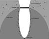 |
Fig. 1. Schematic of the toy model for the acceleration of astrophysical jets. The black arrows show the movement of the gas around the BH and jet. |
 (1)
(1)
where z is the distance from the BH, s is the power-law index of the external pressure (p ∝ z−s), and ωLC = c/Ω = c/0.5Ωh is the cylindrical radius of the light cylinder, where c is the speed of light, and Ωh the angular velocity of the BH (Komissarov et al. 2009; Lyubarsky 2009; Boettcher et al. 2012 and references therein). According to the toy model the maximum Γ is reached at the Bondi radius, i.e.,  , where G is the gravitational constant, M the mass of the BH, and ν∞ the sound speed at the Bondi radius. Then,
 (2)
(2)
The angular velocity of the BH is defined as (3)
(3)
where  , and a is the dimensionless spin of the BH. Assuming a mean molecular weight μ = 0.6 and temperature T = 6.5 × 10⁶ K (consistent with observations of M 87, Narayan & Fabian 2011; Russell et al. 2015) the sound speed at the Bondi radius becomes
 (4)
(4)
Equation (5) is independent of the BH mass which is a necessary condition since similar mass BHs in different systems (i.e micro-quasars and GRBs) produce jets with up to two orders of magnitude different Γ. Γmax depends only on the spin of the BH and the gradient of the external pressure, with Γ having a stronger dependence on the latter. For example, assuming s = a = 0.9, Eq. (5) yields Γmax ≈ 17.24. For a 10% change in a there is a 7.6% change in Γmax, while a 10% change in s results in a 33% change in Γmax. Thus there is only a mild dependence of Γmax on the spin.
3. Application to blazar jets
Studies on the spin and external pressure gradient of beamed sources are extremely rare and in the majority of cases unfeasible. The only source will available estimates for all three parameters that enter Eq. (5) is M 87. Studies of M 87 have determined that the gradient of the external pressure has a power-law index of s = 0.6 (Stawarz et al. 2006); the maximum velocity of the jet at HST-1 is Γmax = 7.21±1.12 (Wang & Zhou 2009); and the BH has a spin of  (Feng & Wu 2017). Using any pair of the above parameters Eq. (5) would yield the third within the uncertainties. Thus the model can produce values consistent with all three observed properties of the jet of M 87.
Although we lack estimates of the a and s for blazars, we were able to use their observed Γ (under the assumption that it is equal to Γmax) to constrain the distributions of the spin and the gradient of the external pressure. There are 75 blazar jets with available Γ estimates (Hovatta et al. 2009; Liodakis et al. 2017; hereafter H09 and L17 respectively) 18 of which are BL Lac objects (BL Lacs) and 57 are flat spectrum radio quasars (FSRQ). These estimates are derived using variability Doppler factors (H09, L17) and apparent velocity estimates (Lister et al. 2009, 2013).
We assumed a distribution for a and s and use the observed Γmax of blazars to constrain the optimal parameters for these distributions using a chi-square (χ2) minimization procedure. For a, since it is bounded between [0, 1] a beta distribution is the natural choice1. For s we tested a normal, a log-normal and a uniform distribution. The distributions (and their parameters) that yielded the lowest reduced χ2 value are shown in Table 1. The results of the minimization were verified using the Kolmogorov–Smirnov (K–S) test2. Figure 2 shows the cumulative distribution function for the observed and simulated Γ max for both blazar populations.
Parameters of the best-fit distributions of a, s for BL Lacs and FSRQs.
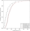 |
Fig. 2. Cumulative distribution function for the observed and simulated Γmax. Black triangles are for the observed BL Lacs and red stars for the observed FSRQs. The dashed black and red lines are the simulated sample for BL Lacs and FSRQs respectively. |
The best-fit distributions for a and s are different for BL Lacs and FSRQs. For the spin, BL Lacs have generally larger spins with a mean of μ = 0.937 while FSRQs have a mean of μ = 0.742. It has been shown analytically that for spin values a < 0.6 the BZ mechanism is no longer efficient (Maraschi et al. 2012). In order to account for the observed γ-ray emission of blazars Maraschi et al. (2012) constrained the spin of blazars to a > 0.5, possibly as high as a ~ 0.8. Cosmological simulations of both BL Lacs and FSRQs have also determined that a sharp cut-off in the spin distribution of blazars is necessary in order to reproduce the number of observed sources in the Universe (Gardner & Done 2014, 2018). Roughly 99.6% of BL Lacs and 80.5% of FSRQs in our sample have a > 0.6. In addition, BL Lacs peak at a ~ 0.9 and FSRQs at a ~ 0.8 showing that our model naturally reproduces the results from different energetic and cosmological perspectives.
For the gradient of the external pressure, the BL Lacs follow a normal, while the FSRQs a log-normal distribution. The FSRQ distribution is also centered at, and extends to, higher values. This would suggest that, on average, the environment in the vicinity of the BHs of FSRQs is denser and therefore more gas-rich than the environment in the vicinity of the BHs in BL Lacs. Environmental conditions have been invoked in the past to explain the dichotomy between FR I and FR II type galaxies (the parent population of BL Lacs and FSRQs respectively). The results of the model would be consistent with evolutionary scenarios that attribute the differences in the two populations (BL Lacs & FSRQs) to differences in their respective accretion rates (e.g., Böttcher & Dermer 2002; Cavaliere & D’Elia 2002; Ajello et al. 2014). If this is the case, then the fact that BL Lacs show on average higher spins would suggest that their BHs were spun up in the past either by accretion of gas that is now depleted (suggesting that BL Lacs are more evolved blazars than FSRQs) or by gas-poor mergers (e.g., Volonteri et al. 2005, 2007, Fanidakis et al. 2011) suggesting a different evolutionary track than FSRQs. The derived values for s are swallower than predicted for Bondi accretion. They are, however, consistent with observations of M 87 (Stawarz et al. 2006) and are, for example, expected in the case were a ion torus supporting the jet is extending outwards from the supermassive BH (Rees et al. 1982).
In order to constrain the values for a and s for individual sources, we draw random values from the optimized distributions for a, s for each population and minimize the square of the difference between observed Γmax and the expectation from the toy model ([ΓObs − Γmodel]2). Table B.1 lists the optimal pairs of a, s that reproduced the observed Γmax after 105 random draws. It should be noted that given the mild dependence of Γmax on the spin, the values of s are better constraint. Nearby sources with large viewing angles (e.g., J1221+2813, L17) could be used to test the predictions of the model for the gradient of the external pressure.
4. Discussion and conclusions
For the application of our model on blazars we used Γ estimates from radio observations. These estimates were derived using a wide range of observing frequencies from 2.6 to 43 GHz (H09, L17). The radio frequency necessary to probe the region where the Γmax is achieved dependents on the properties of source. Results from the MOJAVE survey would suggest that more than half of the blazar jets show accelerating features at 15 GHz (Homan et al. 2015; Lister et al. 2016). Multiwavelength radio observations are then necessary to determine where and whether the Γmax has been reached. For sources whose radio components show significant acceleration at the radio frequency where the Doppler factor (and hence Γ) was derived, the results of the model should be treated as lower limits.
Beyond the Bondi radius we have assumed that the jet has a conical geometry. This might not always be the case. Observations of M 87 do support that scenario (Asada & Nakamura 2012; Asada et al. 2014). MHD simulations have also shown that beyond the recollimation shock at the Bondi radius the jet could become conical, however, depending on the pressure and density profile of the medium outside the Bondi radius different geometries are possible. The resulting geometry could have an impact on the velocity profile of the jet at large scales (e.g., Barniol Duran et al. 2017). Observations of additional AGN jet environments could give more insights on the fate of the jet beyond the Bondi radius.
Throughout this work, we have assumed that the earliest the jet would reach σ ~ 1 is at the Bondi radius. It is, however, possible for the jet to cease being Poynting dominated before reaching the radio core. In such a case the results of the model should be treated as upper limits. We have also assumed that the jet comprises of one bulk flow. It is possible that the Lorentz factor can also change transversely along the jet. Observations of high synchrotron peaked (HSP) sources in the TeV band have shown variability timescales which would require much larger Doppler factors than the ones derived from radio observations. In order to explain this discrepancy, Ghisellini et al. (2005) suggested a spine-sheath configuration: a fast inner spine responsible for the high-energy emission and a slower outer sheath. In this configuration, Ghisellini et al. (2005) found that the spectral energy distribution of four sources can be well described if the sheath has a Γ = [3, 3.5] and the spine a Γ = [15, 17]. If such is the case for blazar jets then the radio observations (which probe the scales at which the Γmax is reached) will be dominated by emission from the sheath (Sikora et al. 2016). Although there are alternate hypothesis to the spine-sheath configuration that can fully explain the observed high energy emission without the need to invoke a faster bulk flow than the one derived from radio observations (e.g., magnetic reconnection, Giannios et al. 2009, 2010) the model can be easily extended to incorporate different flow configurations.
In this work we have presented a simple toy model for the structure and acceleration of jets from supermassive BHs and its application using observed Γ estimates of blazars. Our findings can be summarized as follows:
-
Application to M 87 showed that the model can produce consistent values with all three properties of the jet derived independently from observations.
-
BL Lacs have on average higher spins than FSRQs, with both populations having the vast majority of sources with a > 0.6 consistent with energetic considerations for the efficiency of the BZ mechanism as well as cosmological simulations.
-
The results for the distribution of s in BL Lacs and FSRQs would suggest that the BHs of the latter are, on average, in gas-richer and denser environments than the BHs of the former consistent with evolutionary models that attribute the differences of the two populations in their respective accretion rates.
Although there are many different aspects of the jets that have not been taken into account (MHD instabilities, energy conversion and dissipation mechanisms etc.), the fact that the model can produce consistent results with the observed properties of M 87 as well as the general properties of blazars would suggest that it is a good first approximation on which a more complex and realistic model could be built.
Although different BHs are generally expected to have different spins, given the mild dependence of Γmax on a we also tested a delta function for the spin. The best-fit a for both populations is a ≈ 0.72. Even with the fewer degrees of freedom, the beta distribution still yielded, albeit marginally, a better model according to the reduced χ2. The K–S test also favors the beta distribution over the delta function.
The K–S test yields the probability of two samples being drawn from the same distribution. We do not reject the null hypothesis for any p-value >5%.
Acknowledgments
The author would like to thank the anonymous referee, Rodolfo Barniol Duran, Roger Blandford, Vasiliki Pavlidou, and Roger Romani for comments and discussions that helped improve this work.
References
- Ajello, M., Romani, R. W., Gasparrini, D., et al. 2014, ApJ, 780, 73 [NASA ADS] [CrossRef] [Google Scholar]
- Asada, K., & Nakamura, M. 2012, ApJ, 745, L28 [NASA ADS] [CrossRef] [Google Scholar]
- Asada, K., Nakamura, M., Doi, A., Nagai, H., & Inoue, M. 2014, ApJ, 781, L2 [NASA ADS] [CrossRef] [Google Scholar]
- Barniol Duran, R., Tchekhovskoy, A., & Giannios, D. 2017, MNRAS, 469, 4957 [NASA ADS] [CrossRef] [Google Scholar]
- Begelman, M. C. 2014, ArXiv e-prints [arXiv:1410.8132] [Google Scholar]
- Belczynski, K., Bulik, T., Fryer, C. L., et al. 2010, ApJ, 714, 1217 [NASA ADS] [CrossRef] [Google Scholar]
- Blandford, R. D., & Znajek, R. L. 1977, MNRAS, 179, 433 [NASA ADS] [CrossRef] [Google Scholar]
- Boccardi, B., Krichbaum, T. P., Bach, U., et al. 2016, A&A, 585, A33 [NASA ADS] [CrossRef] [EDP Sciences] [Google Scholar]
- Boettcher, M., Harris, D. E., & Krawczynski, H. 2012, Relativistic Jets from Active Galactic Nuclei (Berlin: Wiley) [CrossRef] [Google Scholar]
- Böttcher, M., & Dermer, C. D. 2002, ApJ, 564, 86 [NASA ADS] [CrossRef] [Google Scholar]
- Cavaliere, A., & D’Elia, V. 2002, ApJ, 571, 226 [NASA ADS] [CrossRef] [Google Scholar]
- Curtis, H. D. 1918, Publications of Lick Observatory, 13, 9 [Google Scholar]
- Daly, R. A., & Marscher, A. P. 1988, ApJ, 334, 539 [NASA ADS] [CrossRef] [Google Scholar]
- Di Matteo, T., Allen, S. W., Fabian, A. C., Wilson, A. S., & Young, A. J. 2003, ApJ, 582, 133 [NASA ADS] [CrossRef] [Google Scholar]
- Fanidakis, N., Baugh, C. M., Benson, A. J., et al. 2011, MNRAS, 410, 53 [NASA ADS] [CrossRef] [Google Scholar]
- Feng, J., & Wu, Q. 2017, MNRAS, 470, 612 [NASA ADS] [CrossRef] [Google Scholar]
- Gardner, E., & Done, C. 2014, MNRAS, 438, 779 [NASA ADS] [CrossRef] [Google Scholar]
- Gardner, E., & Done, C. 2018, MNRAS, 473, 2639 [NASA ADS] [CrossRef] [Google Scholar]
- Ghisellini, G., Tavecchio, F., & Chiaberge, M. 2005, A&A, 432, 401 [NASA ADS] [CrossRef] [EDP Sciences] [Google Scholar]
- Giannios, D., Uzdensky, D. A., & Begelman, M. C. 2009, MNRAS, 395, L29 [NASA ADS] [CrossRef] [Google Scholar]
- Giannios, D., Uzdensky, D. A., & Begelman, M. C. 2010, MNRAS, 402, 1649 [NASA ADS] [CrossRef] [Google Scholar]
- Gómez, J. L., Martí, J. M., Marscher, A. P., Ibáñez, J. M., & Alberdi, A. 1997, ApJ, 482, L33 [NASA ADS] [CrossRef] [Google Scholar]
- Homan, D. C., Lister, M. L., Kovalev, Y. Y., et al. 2015, ApJ, 798, 134 [Google Scholar]
- Hovatta, T., Valtaoja, E., Tornikoski, M., & Lähteenmäki, A. 2009, A&A, 494, 527 [NASA ADS] [CrossRef] [EDP Sciences] [Google Scholar]
- Komissarov, S. S., & Falle, S. A. E. G. 1997, MNRAS, 288, 833 [NASA ADS] [CrossRef] [Google Scholar]
- Komissarov, S. S., Barkov, M. V., Vlahakis, N., & Königl, A. 2007, MNRAS, 380, 51 [NASA ADS] [CrossRef] [Google Scholar]
- Komissarov, S. S., Vlahakis, N., Königl, A., & Barkov, M. V. 2009, MNRAS, 394, 1182 [NASA ADS] [CrossRef] [Google Scholar]
- Komissarov, S. S., Vlahakis, N., & Königl, A. 2010, MNRAS, 407, 17 [NASA ADS] [CrossRef] [Google Scholar]
- Levinson, A., & Globus, N. 2017, MNRAS, 465, 1608 [NASA ADS] [CrossRef] [Google Scholar]
- Liodakis, I., Marchili, N., Angelakis, E., et al. 2017, MNRAS, 466, 4625 [NASA ADS] [CrossRef] [Google Scholar]
- Lister, M. L., Cohen, M. H., Homan, D. C., et al. 2009, AJ, 138, 1874 [NASA ADS] [CrossRef] [Google Scholar]
- Lister, M. L., Aller, M. F., Aller, H. D., et al. 2013, AJ, 146, 120 [NASA ADS] [CrossRef] [Google Scholar]
- Lister, M. L., Aller, M. F., Aller, H. D., et al. 2016, AJ, 152, 12 [NASA ADS] [CrossRef] [Google Scholar]
- Lyubarsky, Y. 2009, ApJ, 698, 1570 [NASA ADS] [CrossRef] [Google Scholar]
- Lyubarsky, Y. E. 2010, MNRAS, 402, 353 [NASA ADS] [CrossRef] [Google Scholar]
- Maraschi, L., Colpi, M., Ghisellini, G., Perego, A., & Tavecchio, F. 2012, J. Phys. Conf. Ser., 355, 012016 [NASA ADS] [CrossRef] [Google Scholar]
- Marscher, A. P. 1995, Proc. Nat. Acad. Sci., 92, 11439 [NASA ADS] [CrossRef] [Google Scholar]
- Marscher, A. P. 2008, ASP Conf. Ser., 386, 437 [Google Scholar]
- Marscher, A. P., Jorstad, S. G., D’Arcangelo, F. D., et al. 2008, Nature, 452, 966 [NASA ADS] [CrossRef] [PubMed] [Google Scholar]
- Marscher, A. P., Jorstad, S. G., Larionov, V. M., et al. 2010, ApJ, 710, L126 [NASA ADS] [CrossRef] [Google Scholar]
- Mertens, F., Lobanov, A. P., Walker, R. C., & Hardee, P. E. 2016, A&A, 595, A54 [NASA ADS] [CrossRef] [EDP Sciences] [Google Scholar]
- Mészáros, P., & Rees, M. J. 2001, ApJ, 556, L37 [NASA ADS] [CrossRef] [Google Scholar]
- Nakamura, M., & Asada, K. 2013, ApJ, 775, 118 [NASA ADS] [CrossRef] [Google Scholar]
- Narayan, R., & Fabian, A. C. 2011, MNRAS, 415, 3721 [NASA ADS] [CrossRef] [Google Scholar]
- Piran, T. 2004, Rev. Mod. Phys., 76, 1143 [NASA ADS] [CrossRef] [Google Scholar]
- Rees, M. J., Begelman, M. C., Blandford, R. D., & Phinney, E. S. 1982, Nature, 295, 17 [NASA ADS] [CrossRef] [Google Scholar]
- Russell, H. R., Fabian, A. C., McNamara, B. R., & Broderick, A. E. 2015, MNRAS, 451, 588 [NASA ADS] [CrossRef] [Google Scholar]
- Sapountzis, K., & Vlahakis, N. 2013, MNRAS, 434, 1779 [NASA ADS] [CrossRef] [Google Scholar]
- Schaerer, D., & Maeder, A. 1992, A&A, 263, 129 [NASA ADS] [Google Scholar]
- Sikora, M., Rutkowski, M., & Begelman, M. C. 2016, MNRAS, 457, 1352 [NASA ADS] [CrossRef] [Google Scholar]
- Stawarz, Ł., Aharonian, F., Kataoka, J., et al. 2006, MNRAS, 370, 981 [NASA ADS] [CrossRef] [Google Scholar]
- Tchekhovskoy, A., McKinney, J. C., & Narayan, R. 2008, MNRAS, 388, 551 [NASA ADS] [CrossRef] [Google Scholar]
- Tchekhovskoy, A., Narayan, R., & McKinney, J. C. 2010, New Ast., 15, 749 [NASA ADS] [CrossRef] [Google Scholar]
- Vlahakis, N. 2004, Ap&SS, 293, 67 [NASA ADS] [CrossRef] [Google Scholar]
- Vlahakis, N. 2015, Astrophys. Space Sci. Lib., 414, 177 [NASA ADS] [CrossRef] [Google Scholar]
- Vlahakis, N., & Königl, A. 2003, ApJ, 596, 1104 [NASA ADS] [CrossRef] [Google Scholar]
- Vlahakis, N., & Königl, A. 2004, ApJ, 605, 656 [NASA ADS] [CrossRef] [Google Scholar]
- Volonteri, M., Madau, P., Quataert, E., & Rees, M. J. 2005, ApJ, 620, 69 [NASA ADS] [CrossRef] [Google Scholar]
- Volonteri, M., Sikora, M., & Lasota, J.-P. 2007, ApJ, 667, 704 [NASA ADS] [CrossRef] [Google Scholar]
- Wang, C.-C., & Zhou, H.-Y. 2009, MNRAS, 395, 301 [NASA ADS] [CrossRef] [Google Scholar]
- Woosley, S. E. 1993, ApJ, 405, 273 [NASA ADS] [CrossRef] [Google Scholar]
Appendix A
Application to gamma-ray bursts
Although the model has been constructed based on observations of jets from supermassive BHs, it would be interesting to explore its application to GRBs. Within the collapsar model (Woosley 1993), the stellar envelope could assume the role of the confining external medium collimating the flow. The jet would then be accelerated in a parabolic geometry until it breaks free from the star envelope to the ISM (Mészáros & Rees 2001). According to Mészáros & Rees (2001)Γ would grow as Γ ∝ z1/2. If this is the case, our model can easily produce Γmax of a few hundreds consistent with the Γ seen in GRBs (e.g., Piran 2004; Begelman 2014). However, the toy model assumes that the end of acceleration takes place at the Bondi radius. In the case of GRBs the end of the jet acceleration would be at the radius (R⋆) of the progenitor star. Then z in Eq. (1) should be substituted with  , where k is the mass ratio of the progenitor star to the resulting BH and depends on the metallicity of the progenitor (Belczynski et al. 2010). Using the mass-to-radius relation for Wolf-rayet stars, R⋆/R⊙ = 10−n(M⋆/M⊙)m, where n = 0.6629 and m = 0.5840 (Schaerer & Maeder 1992) Γmax becomes,
 (A.1)
(A.1)
For similar metallicity progenitors Γmax would depend on the spin of the resulting BH, the pressure profile within the stellar envelope, and the radius of the progenitor star,  . RMHD simulations of GRBs have shown Γmax to have the same dependences (Tchekhovskoy et al. 2008). However, it is also possible for the jet to experience rarefaction acceleration (Tchekhovskoy et al. 2010; Komissarov et al. 2010; Sapountzis & Vlahakis 2013) when exiting the envelope of the progenitor star. If this is the case, the model could only be used to set the initial conditions of the rarefaction acceleration of the jet outside the progenitor star. The fact that the prediction of the model is in agreement with simulations shows some promise, although further investigation into whether this or a similar model is indeed applicable to GRBs is doubtless necessary.
Appendix B
Spin and external pressure gradient estimates
Spin and external pressure gradient estimates for blazars.
All Tables
All Figures
|
Fig. 1. Schematic of the toy model for the acceleration of astrophysical jets. The black arrows show the movement of the gas around the BH and jet. |
| In the text | |
|
Fig. 2. Cumulative distribution function for the observed and simulated Γmax. Black triangles are for the observed BL Lacs and red stars for the observed FSRQs. The dashed black and red lines are the simulated sample for BL Lacs and FSRQs respectively. |
| In the text | |
Current usage metrics show cumulative count of Article Views (full-text article views including HTML views, PDF and ePub downloads, according to the available data) and Abstracts Views on Vision4Press platform.
Data correspond to usage on the plateform after 2015. The current usage metrics is available 48-96 hours after online publication and is updated daily on week days.
Initial download of the metrics may take a while.