© ESO 2018

1. Introduction and nomenclature

When a comet comes sufficiently close to the Sun, it becomes active, releasing volatiles from near-surface layers. Dust grains leave the comet with the gas flow. A coma and a dust tail can be seen by the reflection of sunlight on this dust. The gas in the coma can be ionized, either by particle impact or solar extreme ultraviolet radiation. The ions are eventually picked up by the solar wind, giving rise to an ion tail that is sometimes visible as a result of photon emission in the optical region of the electromagnetic spectrum. In this work we focus on ions within ~100 km from a cometary nucleus. We consider a purely water-dominated coma and assume that all considered species move radially outward with the same velocity u. As the photolysis frequencies are so low for the relevant heliocentric distances (several astronomical units), we may neglect loss of H₂O over the cometocentric distances we consider. We therefore assume that the H₂O number density, n_N, follows a simplified version of the Haser (1957) model:$$n_{\text{N}}\left(r\right)=\frac{Q}{4\pi u{r}^2},$$(1)

where Q is the outgassing rate (the number of H₂O molecules released from the cometary surface per second), u is the expansion velocity (typically on the order of 0.5–1 km s⁻¹), and r is the cometocentric distance. Assuming a constant irradiation level (optically thin medium, which is reasonable at least up to Q values of a few times 10²⁷ s⁻¹, see, e.g., Vigren et al. 2015), the probability that a given H₂O molecule will be ionized on its journey from the surface (at r_c) to r is given by the ionization frequency, f, times the travel time. When the ions move with the same velocity as the neutrals (which we assume throughout this work) and when they are not lost through dissociative recombination, the electron number density, n _e (by quasi-neutrality equal to the total ion number density) is given by$$n_{\text{e}}\left(r\right)=\frac{(r-r_{\text{c}})f}{u}{n}_{\text{N}}\left(r\right)\mathrm{.}$$(2)

While Eq. (2) is a handy analytical expression for predicting the total ion number density at any cometocentric distance given a local measurement of the neutral density and an estimate of the expansion velocity, it holds no information about the ion composition. The photo- or electron-impact ionization of H₂O leads with different branching fractions to H₂O⁺, OH⁺, O⁺, or H⁺ (e.g., Huebner et al. 1992; Vigren et al. 2015; Itikawa & Mason 2005); we consider here branching fractions of 0.703, 0.197, 0.011, and 0.088, respectively. Reactions of these ions with H₂O will affect the relative abundances of the different ion species. The five reactions considered in this work (note that we here only write out the ionic product) are H⁺ + H₂O → H₂O⁺, O⁺ + H₂O → H₂O⁺, OH⁺ + H₂O → H₂O⁺, OH⁺ + H₂O → H₃O⁺, and H₂O⁺ + H₂O → H₃O⁺. Rate coefficients, which are on the order of 10⁻⁹ cm³s⁻¹, may be found at www.udfa.net (McElroy et al. 2013). We use values at 300 K.

We start in Sect. 2 by briefly describing a standard approach of cometary ionospheric modelling as used, for example, by Giguere & Huebner (1978), Vigren & Galand (2013) and Heritier et al. (2017). We note that while details differ in these works, they all work in “r bins” from the surface and outward, and numerically solve a system of coupled differential equations (continuity equations) in each bin. In Sect. 3 we present a different approach that is based on probability arguments. The advantages and disadvantages of the new method compared with the standard method are discussed in Sect. A, together with some concluding remarks. Table 1 summarizes essential parameters of the work.

2. Standard method

The method is used in Vigren & Galand (2013), for example, and is described here only briefly. For a radially expanding coma (and constant expansion velocity u), the continuity equation for ion species i at r is given by$$\frac{\partial n_i(r,t)}{\partial t}+\frac{1}{r^2}\frac{\partial }{\partial r}\left(r^2{n}_i(r,t)u\right)=P_i(r,t)-L_i(r,t)n_i(r,t),$$(3)

where P_i is the production term and L_i is the chemical loss rate of i. In the case of a pure water coma and where loss through dissociative recombination is negligible, we have$$\{\begin{array}{ll}{P}_0(r,t)=\hfill & n_{\text{N}}(r)f_0\hfill \\ P_1(r,t)=\hfill & n_{\text{N}}(r)f_1\hfill \\ P_2(r,t)=\hfill & n_{\text{N}}(r)f_2\hfill \\ P_3(r,t)=\hfill & n_{\text{N}}(r)[f_3+k_{0,3}{n}_0(r,t)+k_{1,3}{n}_1(r,t)+k_{2,3}{n}_2(r,t)]\hfill \\ P_4(r,t)=\hfill & n_{\text{N}}(r)[k_{2,4}{n}_2(r,t)+k_{3,4}{n}_3(r,t)]\hfill \end{array}$$(4)

and$$\{\begin{array}{ll}{L}_0(r,t)=\hfill & n_{\text{N}}(r)k_{0,3}\hfill \\ L_1(r,t)=\hfill & n_{\text{N}}(r)k_{1,3}\hfill \\ L_2(r,t)=\hfill & n_{\text{N}}(r)[k_{2,3}+k_{2,4}]\hfill \\ L_3(r,t)=\hfill & n_{\text{N}}(r)k_{3,4}\hfill \\ L_4(r,t)=\hfill & 0.\hfill \end{array}$$(5)

The numerical solution of the system consists of dividing the coma into spherical shells where densities are assumed to be constant. In the innermost shell, there is no ion inflow from below. A set of initial ion number densities (close to zero) is set in the innermost shell, and the equation system is run with an appropriate (low) time step until convergence (according to a predefined criterion) is reached. Thereafter, the second shell is considered, now accounting for the ion inflow from below and using as initial densities the “final” densities in the shell below. The procedure continues through all shells.

3. New method

The arrival of an H⁺, O⁺, or OH⁺ ion at r requires that an H₂O molecule has undergone dissociative ionization at some point r′ and that the resulting ion avoid reactions with H₂O molecules on its way from r′ to r. The probability expression becomes (i = 0, 1, 2)$$K_i\left(r\right)={\int }_{r_{\mathrm{c}}}^r\frac{f_i}{u}\exp \left({\eta }_i[\frac{1}{r}-\frac{1}{r\prime }]\right)\mathrm{d}r\prime ,$$(6)

with parameters as described in Table 1, but we recall that$${\eta }_i=\frac{Q{k}_i}{4\pi u^2}\mathrm{.}$$(7)

For guidance, the factor _fidr′/u in Eq. (6) corresponds to the probability that a neutral molecule is ionized into ion species i during the time interval dt = dr′/u and the exponential factor represents the probability, P(r,r′), for an ion “born” at r′ to reach r without undergoing reactions during the journey. We note that dP/P = −k_in_Ndr″/u = −η_idr″/r″². Using the chain rule, we arrive at the relation d(ln P)/dr″ = − η_i/r″². Integration then gives ln(P(r,r′)) – ln(P(r′, r′)) = η_i(1/r–1/r′), and since P(r′,r′) = 1 and ln 1 = 0, we obtain the desired relation P(r, r′) = exp(η_i(1/r–1/r′)). The integral in Eq. (6) is readily evaluated as (see Appendix A)$$K_i\left(r\right)=\frac{f_i}{u}\{r-r_{\mathrm{c}}\exp \left({\eta }_i[\frac{1}{r}-\frac{1}{r_{\mathrm{c}}}]\right)+{\eta }_i\left[E\left(\frac{{\eta }_i}{r_{\mathrm{c}}}\right)-E\left(\frac{{\eta }_i}{r}\right)\right]\exp \left(\frac{{\eta }_i}{r}\right)\},$$(8)

where we have defined the exponential integral as$$E\left(x\right)={\int }_x^{\infty }\frac{\exp (-t)}{t}\mathrm{d}t\mathrm{.}$$(9)

The arrival of an H₂O⁺ ion at r requires either (i) that an H₂O molecule undergo non-dissociative ionization at some point r′ and that the resulting H₂O⁺ ion avoid reactions with H₂O molecules on its way from r′ to r, or (ii) that an H⁺, O⁺ or OH⁺ ion reaches r′ where it reacts with H₂O to produce H₂O⁺, which in turn avoids reactions with H₂O molecules on its way from r′ to r. The resulting probability expression becomes$$K_3\left(r\right)=\frac{f_3}{u}{\int }_{r_{\mathrm{c}}}^r\exp \left({\eta }_3[\frac{1}{r}-\frac{1}{r\prime }]\right)\mathrm{d}r\prime +\underset{i=0}{\overset{2}{\mathrm{\Sigma }}}\frac{k_{i,3}}{u}{\int }_{r_{\mathrm{c}}}^r{K}_i(r\prime )n_{\mathrm{N}}(r\prime )\exp \left({\eta }_3[\frac{1}{r}-\frac{1}{r\prime }]\right)\mathrm{d}r\prime \mathrm{.}$$(10)

In compact notation, we may express this as$$K_3\left(r\right)=K_{3\to 3}\left(r\right)+K_{0\to 3}\left(r\right)+K_{1\to 3}\left(r\right)+K_{2\to 3}\left(r\right),$$(11)

where the indexing shows the pathway to H₂O⁺, for instance, 2 → 3 means that it proceeds via OH⁺. We have from Eq. (8) that$$K_{3\to 3}\left(r\right)=\frac{f_3}{u}\{r-r_{\mathrm{c}} \exp \left({\eta }_3[\frac{1}{r}-\frac{1}{r_{\mathrm{c}}}]\right)+{\eta }_3[E\left(\frac{{\eta }_3}{r_{\mathrm{c}}}\right)-E\left(\frac{{\eta }_3}{r}\right)]\exp (\frac{{\eta }_3}{r}\left)\right\}\mathrm{.}$$(12)

For i = 0, 1, 2 one can from Eqs. (8) and (10) arrive at$$K_{i\to 3}\left(r\right)=\frac{f_{i}Q{k}_{i,3}}{4\pi u^3}\{A_i\left(r\right)-r_{\mathrm{c}}{B}_i\left(r\right)+{\eta }_{i}E\left(\frac{{\eta }_i}{r_{\mathrm{c}}}\right)C_i\left(r\right)-{\eta }_i{D}_i\left(r\right)\},$$(13)

where A_i, B_i, C_i, and D_i represent four integrals similar to Eq. (10) thatcanbeevaluatedbystandardmethods(e.g.,Geller & Ng1969) to yield (for i = 0, 1, 2)$$A_i\left(r\right)=\exp \left(\frac{{\eta }_3}{r}\right)\left[E\right(\frac{{\eta }_3}{r})-E(\frac{{\eta }_3}{r_{\mathrm{c}}}\left)\right]$$(14) $$B_i\left(r\right)=\frac{1}{{\alpha }_i}\exp (\frac{{\eta }_3}{r}-\frac{{\eta }_i}{r_{\mathrm{c}}})[\exp (\frac{{\alpha }_i}{r_{\mathrm{c}}})-\exp (\frac{{\alpha }_i}{r}\left)\right]$$(15) $$C_i\left(r\right)=\frac{1}{{\alpha }_i}\exp \left(\frac{{\eta }_3}{r}\right)[\exp (\frac{{\alpha }_i}{r_{\mathrm{c}}})-\exp (\frac{{\alpha }_i}{r}\left)\right]$$(16) $$D_i\left(r\right)=\frac{1}{{\alpha }_i}\exp \left(\frac{{\eta }_3}{r}\right)[E(\frac{{\eta }_3}{r})-E(\frac{{\eta }_3}{r_{\mathrm{c}}})+\exp \left(\frac{{\alpha }_i}{r_{\mathrm{c}}}\right)E\left(\frac{{\eta }_i}{r_{\mathrm{c}}}\right)-\exp \left(\frac{{\alpha }_i}{r}\right)E\left(\frac{{\eta }_i}{r}\right)],$$(17)

where (for i = 0, 1, 2)$${\alpha }_i={\eta }_i-{\eta }_3\mathrm{.}$$(18)

Equations (10)–(18) allow calculation of K₃(r). We then have for i = 0, 1, 2, 3$$n_i\left(r\right)=n_{\mathrm{N}}{\left(r\right)K}_i\left(r\right)$$(19)

and for i = 4, that is, H₃O⁺,$$n_4\left(r\right)=n_e\left(r\right)-\underset{i=0}{\overset{3}{\mathrm{\Sigma }}}{n}_i\left(r\right),$$(20)

where n_e(r) is given by Eq. (2).

4. Discussion and conclusions

We have tested the two methods against each other and obtained good agreement (see Fig. 1 for a case example) where minor deviations (seen only near the surface) are due to the errors associated with the use of discrete time and altitude steps in the standard method. The new method is extremely fast. It does not include time steps, and it can generate densities at a given r without first having to calculate densities closer to the nucleus. These are the main advantages of the new method. A further advantage with closed-form expressions is that it allows us to see how different terms scale and how the densities evolve in different limits.

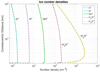Fig. 1. Ion number densities calculated from the standard model (colored lines) and from the analytical model (overplotted dashed lines). For these simulation Q = 2 × 1026 s−1 and u = 600 m s−1. Discrepancies near the surface are attributed to the discrete altitude levels and time steps considered in the standard method.

The new method also has disadvantages. It is set up based on simplifying assumptions such as a constant expansion velocity, constant ionization frequencies, constant reaction rate coefficients, and the assumption that dissociative recombination (leading to removal of ions) is negligible. The standard method can accomodate varying parameters as well as dissociative recombination. Still, the analytical approach can be used as a limiting test for numerical codes. Another disadvantage of the new method is that it requires much more effort in order to implement an extended set of neutrals and associated ions and ion-neutral reactions. For example, if NH₃ were to be added, ${\text{NH}}_4^{+}$ would overtake the role of H₃O⁺ as terminal ion $({\text{H}}_3{\text{O}}^{+}+{\text{NH}}_3\to {\text{NH}}_4^{+})$, and the derivation of an analytical expression for the density of H₃O⁺ would have to include pathways involving two binary reactions. With the addition of more species, the number of ion production pathways increases, and some of the pathways can include many reaction steps. While in principle analytical solutions are there, they may be tedious to find (or even to implement).

A final limitation of the new method is that when the activity is high, the exponential factors can grow larger than what many solvers can handle. Taylor expansion on multiplications of exponential and E functions may offer a way around such obstacles. However, for activity levels that show this problem, some of the other simplifying assumptions are already highly questionable, and therefore we do not expand on the issue further here. While we here considered a coma dominated by H₂O, it is noted that consideration of a H₂O/CO₂ coma, for instance, might to first approximation be approached using expressions in similar forms as those presented here, and we therefore postpone derivations of closed-form expressions for reaction pathways involving more than one binary reaction to the future. ${\text{CO}}_2^{+}$, the dominant ion produced in the photolysis of CO₂, is non-reactive with CO₂, but reactive with H₂O to mainly form H₂O⁺. Including this chemistry would only result in additional terms in the formalism we have presented. Extended pathways via minor primary ions are not expected to contribute greatly to the build-up of H₂O⁺ (and H₃O⁺), although for detailed comparisons with results from standard models, closed-form expressions for pathways with at least two binary reactions are desirable. The influence of the electric and magnetic field environment is a greater concern; this is not explicitly accounted for in either the standard or the new method we presented here. The ion-neutral decoupling distance as fomulated in Eq. 3 in Mandt et al. (2016; see also their Fig. 5), for example, could give a rough indication of where the model is applicable for a given activity level, but the actual situation is likely very complex. The closed-form expressions presented here offer a fast way to compare model-derived relative ion abundances with observations from ROSINA/DFMS measurements (e.g., Fuselier et al. 2016; Heritier et al. 2017) in the coma of comet 67P/Churyumov-Gerasimenko, the target comet of the Rosetta mission. Marked variations in relative ion abundances seen in observations and not captured by the model could give important clues about spatial and/or temporal variations in the field environment.

Acknowledgments

We thank the Swedish National Space Board for financial support (Dnr 166/14) and Anders Eriksson for valuable discussions. We also acknowledge the International Space Science Institute; this work was done in the framework of the ISSI International Team on the plasma environment of comet 67P after Rosetta, number 402.

References

Appendix A

Evaluation of Eq. (6)

We note that Eq. (6) can be rewritten in the form$$K_i\left(r\right)=A{\int }_{r_{\mathrm{c}}}^r\exp (-\frac{{\eta }_i}{r\prime })\mathrm{d}r\prime ,$$(A.1)

where A = (f_i/u)exp(η_i/r). We can integrate by parts to obtain$$K_i\left(r\right)/A=r \exp (-\frac{{\eta }_i}{r})-r_{\mathrm{c}} \exp (-\frac{{\eta }_i}{r_{\mathrm{c}}})-{\int }_{r_{\mathrm{c}}}^r\frac{{\eta }_i}{r\prime }\exp (-\frac{{\eta }_i}{r\prime })\mathrm{d}r\prime \mathrm{.}$$(A.2)

For the latter integral, we make the variable substitution η_i/r′ = t so that dr′= η_idt/t² and$$K_i\left(r\right)/A=r \exp (-\frac{{\eta }_i}{r})-r_{\mathrm{c}} \exp (-\frac{{\eta }_i}{r_{\mathrm{c}}})-{\eta }_i {\int }_{{\eta }_i/r}^{{\eta }_i/r_{\mathrm{c}}}\frac{1}{t}\exp (-t)\mathrm{d}t,$$(A.3)

where we have taken care of a sign by switching the integration limits. We realize that$${\int }_{{\eta }_i/r}^{{\eta }_i/r_{\mathrm{c}}}\frac{1}{t}\exp (-t)\mathrm{d}t= {\int }_{{\eta }_i/r}^{\infty }\frac{1}{t}\exp (-t)\mathrm{d}t-{\int }_{{\eta }_i/r}^{\infty }\frac{1}{t}\exp (-t)\mathrm{d}t\mathrm{.}$$(A.4)

From Eqs. (9) and (A.4), we see that$${\int }_{{\eta }_i/r}^{{\eta }_i/r_{\mathrm{c}}}\frac{1}{t}\exp (-t)\mathrm{d}t=E({\eta }_i/r)-E({\eta }_i/r_{\mathrm{c}})\mathrm{.}$$(A.5)

Inserting this into Eq. (A.3) and applying some trivial algebra yields the desired Eq. (8).

All Tables

All Figures

	Fig. 1. Ion number densities calculated from the standard model (colored lines) and from the analytical model (overplotted dashed lines). For these simulation Q = 2 × 1026 s−1 and u = 600 m s−1. Discrepancies near the surface are attributed to the discrete altitude levels and time steps considered in the standard method.
In the text

References

- Fuselier, S. A., Altwegg, K., Balsiger, H., et al. 2016, MNRAS, 462, S67 [NASA ADS] [CrossRef] [EDP Sciences] [Google Scholar]
- Geller, M., & Ng, E. W. 1969, J. Res. Nat. Bur. Stand. B. Math. Sci., 73, 191 [CrossRef] [Google Scholar]
- Giguere, P. T., & Huebner, W. F. 1978, ApJ, 223, 638 [NASA ADS] [CrossRef] [Google Scholar]
- Haser, L. 1957, In Bulletin de la Classe de Science, Académie Royale de Belgique, 43, 740 [Google Scholar]
- Heritier, K. L., Altwegg, K., Balsiger, H., et al. 2017, MNRAS, 469, S427 [Google Scholar]
- Huebner, W. F., Keady, J. J., & Lyon, S. P. 1992, Ap&SS, 195, 1 [NASA ADS] [CrossRef] [Google Scholar]
- Itikawa, Y., & Mason, N. 2005, J. Phys. Chem. Ref. Data, 34, 1 [NASA ADS] [CrossRef] [Google Scholar]
- Mandt, K. E., Eriksson, A. I., Edberg, N. J. T., et al. 2016, MNRAS, 462, S9 [NASA ADS] [CrossRef] [Google Scholar]
- McElroy, D., Walsh, C., Markwick, A. J., et al. 2013, A&A, 550, A36 [NASA ADS] [CrossRef] [EDP Sciences] [Google Scholar]
- Vigren, E., & Galand, M. 2013, ApJ, 772, 33 [Google Scholar]
- Vigren, E., Galand, M., Eriksson, A. I., et al. 2015, ApJ, 812, 54 [NASA ADS] [CrossRef] [Google Scholar]