| Issue |
A&A
Volume 616, August 2018
|
|
|---|---|---|
| Article Number | A134 | |
| Number of page(s) | 7 | |
| Section | The Sun | |
| DOI | https://doi.org/10.1051/0004-6361/201732323 | |
| Published online | 31 August 2018 | |
Reconstructing solar magnetic fields from historical observations
III. Activity in one hemisphere is sufficient to cause polar field reversals in both hemispheres
1
ReSoLVE Centre of Excellence, Space Climate research unit, University of Oulu, PO Box 3000, 90014 Oulu, Finland
e-mail This email address is being protected from spambots. You need JavaScript enabled to view it.
2
National Solar Observatory, Boulder, CO 80303, USA
Received:
20
November
2017
Accepted:
24
May
2018
Abstract
Aims. Sunspot activity is often hemispherically asymmetric, and during the Maunder minimum, activity was almost completely limited to one hemisphere. In this work, we use surface flux simulation to study how magnetic activity limited only to the southern hemisphere affects the long-term evolution of the photospheric magnetic field in both hemispheres. The key question is whether sunspot activity in one hemisphere is enough to reverse the polarity of polar fields in both hemispheres.
Methods. We simulated the evolution of the photospheric magnetic field from 1978 to 2016 using the observed active regions of the southern hemisphere as input. We studied the flow of magnetic flux across the equator and its subsequent motion towards the northern pole. We also tested how the simulated magnetic field is changed when the activity of the southern hemisphere is reduced.
Results. We find that activity in the southern hemisphere is enough to reverse the polarity of polar fields in both hemispheres by the cross-equatorial transport of magnetic flux. About 1% of the flux emerging in the southern hemisphere is transported across the equator, but only 0.1%–0.2% reaches high latitudes to reverse and regenerate a weak polar field in the northern hemisphere. The polarity reversals in the northern hemisphere are delayed compared to the southern hemisphere, leading to a quadrupole Sun lasting for several years.
Key words: Sun: activity / Sun: magnetic fields / Sun: photosphere
© ESO 2018
1. Introduction
Understanding the nature of the solar cycle is one of the fundamental questions of solar physics. The widely accepted phenomenological concept of the solar cycle, the so-called Babcock-Leighton model (Babcock 1961; Leighton 1969), describes the solar cycle as a transformation of poloidal field, which is concentrated in polar areas at the beginning of each cycle, into toroidal field. As the cycle progresses, increase in toroidal field gives rise to active regions in mid to low latitudes. The magnetic field of dissipating active regions is dispersed by near-surface motions (mostly by superganular flows) and transported across the solar surface by meridional flows. The leading polarity fields of active regions in each hemisphere are transported to the equatorial zone, where they cancel each other, while the trailing polarities are transported poleward, where they reconstruct the poloidal field for the next minimum. Based on the original idea by Ohl (1966) using geomagnetic activity as a proxy of polar fields, the strength of the polar field at solar minimum has been shown to strongly correlate with the amplitude of the following sunspot maximum (Schatten et al. 1978; Petrovay 2010). The Babcock-Leighton model led to the development of surface flux transport (SFT) models, which are now successfully used in modeling the properties of solar cycles. Modern SFT models have been shown to accurately represent the distribution of surface field (Jiang et al. 2014; Yeates et al. 2015; Lemerle et al. 2015); they have been used for various purposes ranging from simulating the long-term evolution of the photospheric field (Jiang et al. 2014; Virtanen et al. 2017) to studying individual flux surges (Yeates et al. 2015).
An SFT model typically includes meridional circulation, differential rotation, diffusion, and a term describing the emerging flux. Previous studies based on SFT models show the importance of certain properties of active regions to the strength of the next solar cycle. A larger tilt of active regions will lead to higher cycles (Baumann et al. 2004). The speed of the meridional flow may have a significant impact on the polar field, which determines the strength of the next cycle (Hathaway & Upton 2014; Upton & Hathaway 2014). Emerging flux can be treated in many different ways. Typically, active regions are added to the simulation at certain points in time to represent flux emergence. Active regions can be constructed from sunspot observations (Sheeley et al. 1985; Schrijver et al. 2002; Baumann et al. 2004; Jiang et al. 2010, 2011), or they can be assimilated from magnetograms (Worden & Harvey 2000; Yeates et al. 2015; Virtanen et al. 2017).
Despite the many studies, the main property of the Babcock-Leighton model, the approximate hemispheric symmetry of flux emergence, has not been challenged (Hathaway & Upton 2016). The Babcock-Leighton model assumes that the magnetic flux of the leading polarity fields of active regions cancels out across the solar equator. This leaves several important questions open. What would be the effect on the solar cycle if sunspot activity was strongly asymmetric hemispherically, or was even completely restricted to one hemisphere only? Would we still see the build-up of the poloidal field in polar areas in both hemispheres, or would the alternation of the polarity of polar fields as a signal of the solar 22-yr magnetic (Hale) cycle be disrupted?
Sunspot activity is hemispherically asymmetric in most solar cycles. For example, the current cycle 24 is strongly asymmetric. Relatively, even a stronger asymmetry occurred during the Maunder minimum in the second half of the 17th century. While sunspots were very rare during this time, observations recorded at the Observatoire de Paris show that the small number of sunspots that were observed appeared almost exclusively in the southern hemisphere (Ribes & Nesme-Ribes 1993).
In this paper, we use an SFT simulation to study the effect of having new flux emerging in the southern hemisphere only. We examine whether activity in one hemisphere is enough to develop polar fields in both hemispheres and to reverse their polarity from cycle to cycle. We also estimate the magnitude of the cross-equatorial transport of magnetic flux and follow the evolution of this flux as it travels towards the northern pole. Finally we test how reducing the amount of emerging flux in the southern hemisphere affects the simulated polar fluxes. The paper is organized as follows. In Sect. 2, we describe the synoptic maps used as input in simulations, and in Sect. 3 we give a short description of the SFT model and its main parameters. In Sect. 4, we present the simulated magnetic fields. In Sect. 5, we study the cross-equatorial transport of flux. In Sect. 6, we investigate how reducing the amount of emerging flux in the southern hemisphere affects the simulations, and in Sect. 7 we give our conclusions.
2. Observations and super-synoptic maps
The photospheric line-of-sight magnetic field has been measured at the National Solar Observatory (NSO) Kitt Peak (KP) observatory since the early 1970s. From February 1974 (Carrington rotation (CR) 1625) until March 1992 (CR 1853) the instrument was a 512-channel diode array magnetograph using the Fe I 868.8 nm spectral line (Livingston et al. 1976). The CCD spectromagnetograph (SPMG) started operating in 1992, first using the Fe I 550.7 nm spectral line from April to October 1992 (CR 1855–1862) and thereafter the same Fe I 868.8 nm line as the previous instrumentation (Jones et al. 1992). These observations terminated in August 2003 (CR 2006), when the Synoptic Optical Long term Investigations of the Sun (SOLIS) vector spectromagnetograph (VSM) replaced the old instrumentation (Keller et al. 2003). In 2006, the VSM modulators were replaced, and in 2010, the original Rockwell cameras, which had a pixel size of 1.125″, were replaced by Sarnoff cameras that have a smaller pixel size of 1″ (Pietarila et al. 2013).
These observations are used to create pseudo-radial synoptic maps with a resolution of one degree in longitude and 1/90 in sine of latitude. The same data were used in our previous study (Virtanen et al. 2017, see additional details about the data there). Figure 1 shows the combined KP and SOLIS data sets in 1978–2016 in the form of the so-called super-synoptic (or magnetic butterfly) map. Each vertical line was formed by averaging a synoptic map over longitude. The switch from the earlier Kitt Peak instrumentation to SOLIS happened in August 2003 between rotations 2006 and 2007. Data gaps (white in Fig. 1) were not filled. Therefore, no active regions were assimilated into the simulation during rotations with no observations. On July 21, 2014, SOLIS was relocated from Kitt Peak to Tucson, Arizona, leading to the longest data gap.
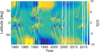 |
Fig. 1. Super-synoptic map of the KP and SOLIS photospheric magnetic field observations from January 1978 (CR 1664) to December 2016 (CR 2184). Yellow and blue colors correspond to positive and negative polarity. White vertical lines are periods with no observations. |
3. Surface flux transport model
The SFT model used in this work is based on the model of Yeates et al. (2015). It has been extended with the decay term of Baumann et al. (2006), which is based on the diffusion of the radial field in the convection layer, and solves the known problem related to the inability of SFT models to reverse the polarity of polar fields correctly during weak cycles, such as cycle 24 (Lean et al. 2002; Schrijver et al. 2002; Baumann et al. 2006; Yeates 2014; Virtanen et al. 2017). Here we use the decay rate derived by Baumann et al. (2006). The model uses the KP and SOLIS synoptic maps, identifies their active regions and assimilates these into the simulation. The model and its sensitivity to parameter values and uncertainties in the input data have recently been tested (Virtanen et al. 2017), and have been found to be robust and suitable for studies of the long-term evolution of the photospheric magnetic field. Only a short description is included here (for a detailed description of the model, see Virtanen et al. 2017).
We write the radial magnetic field Br(θ, ø, t) in the spherical coordinate system in terms of the two-component vector potential [Aθ, Aø]: (1)
(1)
where R is the radius of the Sun, θ is colatitude, ø is the azimuth angle, and t is time. The vector potential evolves in time as follows (Yeates et al. 2015): (2)
(2)
 (3)
(3)
where ω(θ) is the differential angular velocity of rotation, D is the supergranular diffusivity coefficient, and uθ(θ) is the velocity of meridional circulation. Sθ and Sø represent the emergence of new flux in active regions. The active regions are taken from observations and added directly to the simulated radial field.
We used the angular velocity of differential rotation ω(θ) (in the Carrington rotation frame) of Yeates et al. (2015): (4)
(4)
and the semi-empirical meridional circulation profile of Schüssler & Baumann (2006), which has been adapted to helioseismic measurements: (5)
(5)
We used a supergranular diffusion coefficient of D = 400 km2s−1 and a peak meridional circulation speed of u0 = 11 ms−1. The radial magnetic field at the start of the simulation in January 1978 was defined by the synoptic map of CR 1664. The vector potential was evolved in time according to Eqs. (2) and (3). Active regions were added to the simulation when they crossed the central meridian. Optimization of parameter values and identification of active regions are described in detail in Virtanen et al. (2017), and also studied in Whitbread et al. (2017).
The decay term of Baumann et al. (2006) is derived assuming that the magnetic field B is radial at the surface and that the radial component disappears at the bottom of the convection layer at 0.7 R. This leads to the following decay rate E(θ, ø, t) of the radial surface field: (6)
(6)
where Ylm(θ, ø) are spherical harmonics, clm are the harmonic coefficients of the simulated radial field at time t, and τl are the decay times for each harmonic mode l (l = 1–9) shown in Table 1. Modes higher than l = 9 have short decay times and do not affect the long-term evolution of the field.
Decay times τl.
The differential equations are solved with a numerical finite difference method using a time step of about 14 min. Because the decay process is slow and does not require a high time resolution, the decay term is computed and subtracted from the radial field only every 100th time step in order to save computation time.
4. The simulated photospheric field
For a reference, the top panel of Fig. 2 shows a full-activity simulation that includes the active regions from both hemispheres, and the second panel from the top a simulation that includes active regions from both hemispheres but does not include the decay term. As discussed earlier by Virtanen et al. (2017), the simulation including the decay term agrees fairly well with the observed field shown in Fig. 1. There are differences in the polar areas, especially in the 1980s, which are, at least partly, due to errors in the data (Virtanen et al. 2017; Virtanen & Mursula 2016). The long-term evolution of the field, including the timings of polarity reversals, are very similar in the simulation and the observations. The simulation without the decay term starts to deviate significantly from the simulation including the decay term and the observations in the late declining phase of cycle 23. Before that, there is enough activity to cause the evolution of the polar fields to be mostly dictated by flux emergence in both simulations. Without decay, polar fields are slightly stronger, and attain their maxima and reverse their polarity slightly later than with decay, but the overall evolution of the field is still quite similar in the two simulations. However, during the deep minimum between cycles 23 and 24, decay becomes the dominant process, if it is included. Without it, polar fields remain constant, and the emerging flux of the weak cycle 24 is not enough to reverse the polarity.
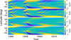 |
Fig. 2. Super-synoptic maps of the photospheric magnetic field from February 1978 (CR 1665) to December 2016 (CR 2184) from simulations using active regions in both hemispheres with the decay term (top panel), in both hemispheres but without the decay term (second panel from the top), only in the southern hemisphere (third panel from the top), and only in the southern hemisphere but without the decay term (bottom panel). |
The hemispherically asymmetric simulation (third panel of Fig. 2) includes only the active regions of the southern hemisphere as input. The northern half of the KP and SOLIS synoptic maps was not included in active region detection. As a result, the only way for flux to enter the northern hemisphere is by transport across the equator. The effect of including active regions of the northern hemisphere in the first synoptic map at the beginning of modeling can be seen over the first few years as a strong and persistent polar field in the northern hemisphere and as one poleward surge of opposite polarity originating at mid-latitudes. However, these traces of the first map disappear rather rapidly, and by about 1985, the original polar field of the northern pole has decayed away. After this time, all changes that are seen in the northern hemisphere are entirely due to the sunspot activity of the southern hemisphere. The similar “loss of memory” was seen earlier (Virtanen et al. 2017), in that the effect of initial conditions on polar fields vanished after about one solar cycle.
Figure 2 (third panel) shows that, even without any new flux emerging in the northern hemisphere, polarity reversals can still be observed even in the northern hemisphere. Since meridional flows are directed poleward in either hemisphere, the only mechanism that can transport magnetic flux across the solar equator is diffusion. The simulation results depicted in Fig. 2 show that cross-equatorial flux transport is quite efficient. Once the magnetic flux has crossed the equator, it can be transported towards the northern pole also by the meridional flow.
As seen in Fig. 2, the northern polar field in the south-activity simulation remains significantly weaker than in the full-activity simulation. Moreover, the development of the northern polar fields, as well as their polarity reversal, are delayed. This is most likely due to flux having to travel a longer distance from the southern hemisphere to the northern pole. Moreover, the meridional circulation is slower at low latitudes than at mid-latitudes where flux is normally generated. This delays the timing of polarity reversals in the northern hemisphere relative to the active southern hemisphere. Accordingly, the polarity reversals in the two opposite poles develop a mutual delay, causing the two hemispheres to evolve systematically asynchronously.
To assess the effect of the decay term, the bottom panel of Fig. 2 shows a south-activity simulation without it. Without decay the polar fields are slightly stronger, and in the north reverse their polarity later than in the south-activity simulation including the decay term. In the northern hemisphere, the polarity reversal of cycle 24 does not happen within the time frame of the simulation, but all other polarity reversals are observed. This shows that while the strength of the polar fields and the timings of polarity reversals depend on the decay term, the south-activity simulation does not require it to reverse polarities in both hemispheres, and the asynchronicity between the hemispheres is in fact stronger without decay.
Figure 3 shows the average intensity of polar fields below −60° and above 60° latitude in the two simulations shown in Fig. 2. The northern polarity reversals of cycles 21–23 occur three to four years later in the south-activity simulation than in the full-activity simulation. For cycle 24, this difference is about two years. The southern polarity reversals happen slightly earlier in the south-activity simulation. The difference is a few months for cycles 21–23 and about a year for cycle 24. This means that also the southern pole is slightly affected by the lack of flux emergence in the northern hemisphere. We also note that, because of the delayed reversal of the northern pole in the south-activity simulation, both poles have the same polarity for three to four years during the early declining phase of each cycle.
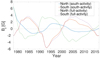 |
Fig. 3. Average field strength above 60° and below −60° latitude from the simulations shown in Fig. 2. |
The northern polar field in the south-activity simulation reaches its peak intensity considerably later than in the full-activity simulation. This difference is about 3 yr for cycle 21 and 4 yr for cycles 22 and 23. However, while the full-activity simulation shows two separate peaks for cycles 22 and 23, the south-activity simulation shows always one maximum only, and a very flat peak for cycle 23, which makes the exact delay rather uncertain. The peaks of the northern polar fields in the south-activity simulation are rather low, reaching −1.4G, 1.6G, and −0.9G during cycles 21, 22, and 23, respectively, while in the full-activity simulation, the corresponding peak values are −3.0G, 3.6G, and −3.8G. This means that the maximum of the northern polar field is more than twice stronger in the full-activity simulation during cycles 21 and 22, and about four times stronger during cycle 23.
Since the timings of polarity reversals in the south are only slightly different in the two simulations, it seems that the flux crossing the equator from the northern to southern hemisphere in the full-activity simulation is not very important for the temporal evolution of the southern polar fields. Also, the field strength of the southern hemisphere is mostly unaffected by the omission of active regions in the northern hemisphere. This is because the southern polar field is formed by trailing flux from the active regions in the southern hemisphere. As the regions disperse, some of the trailing flux is canceled by the leading flux, and the rest is transported poleward, creating the polar field. This process is not strongly affected by active regions in the northern hemisphere. The only significant difference is seen during the declining phase of cycle 23 and the minimum between cycles 23 and 24, when the southern field is considerably weaker in the south-activity than full-activity simulation. This is most likely caused by enhanced cross-equatorial transport of flux of trailing polarity in the south-activity simulation during the declining phase of cycle 23. Because the trailing polarity in the south is the leading polarity in the north, in the full-activity simulation the flows of trailing polarity aiming to cross the equator collide with fields of the same polarity on the other side of the equator. Since the speed of supergranular diffusion depends on the gradient of the field, this effectively stops the flow of the trailing polarity across the equator in the full-activity simulation. However, in the south-activity simulation the trailing polarity flux can cross the equator more freely. Therefore the trailing polarity near the equator is more effectively transported to the northern hemisphere in the south-activity simulation, which weakens both polar fields. This is particularly effective during the long cycle 23, when active regions are located closer to the equator than in the earlier cycles.
5. Cross-equatorial transport
In order to determine how much magnetic flux flows across the equator to the northern hemisphere in the south-activity simulation, we calculated the change of intensity in the row of pixels at the lowest northern latitude. We calculated how much the field in these pixels changes during each time step of the simulation if we ignore supergranular diffusion, differential rotation, and meridional circulation in the northern hemisphere. Turning off diffusion and meridional circulation in the northern hemisphere means that the magnetic flux transported across the equator to the northern hemisphere remains in the lowest northern pixels, since the flux cannot be transported northward, nor will it diffuse to the neighboring pixels. The only process that can change the intensity of the field in these pixels is the cross-equatorial transport caused by diffusion in the southern hemisphere. We summed the field differences over longitude and Carrington rotation, thus obtaining the amount of flux transported over the equator during each rotation. We then repeated the same procedure first at 30° latitude and then at 60° latitude, ignoring supergranular diffusion, differential rotation and meridional circulation north of 30° and 60° latitude, respectively, but taking them into account elsewhere, and computing the field change in the first row of pixels north of the limit.
Figure 4 (three top panels) shows the signed flux transported in a Carrington rotation across three different latitudes. The flow across the equator (top panel) is strongest after the sunspot maximum, in the declining phase, and very weak during the minimum and in the ascending phase. This is to be expected, because active regions at low latitudes are the source of the cross-equatorial flux, and these are most common in the declining phase of the sunspot cycle. We note that the cross-equatorial transport is very irregular. There are strong spikes that correspond to the emergence of large individual active regions near the equator. The sign of the spikes mostly follows the polarity of the leading flux in the southern hemisphere during each solar cycle. However, they can also have an opposite polarity, verifying the cross-equatorial transport of trailing flux. Since the majority of active regions obey Hale’s and Joy’s laws, the average cross-equatorial transport during each solar cycle has the expected polarity. Accordingly, northward flows in the northern hemisphere have a polarity corresponding to the Hale cycle evolution of fields of the southern hemisphere. The same spikiness and alternation of field polarity can be seen in the lower panel of Fig. 2 as narrow surges of positive and negative polarity crossing the equator, for example, in 2002–2003.
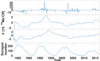 |
Fig. 4. Amount of flux transported northward by supergranular diffusion at the equator (top panel), and by diffusion and meridional circulation at 30° latitude (second panel from the top) and at 60° latitude (third panel from the top). The bottom panel shows the 13-month smoothed monthly sunspot number for reference (SILSO World Data Center 1978–2016). |
The second panel in Fig. 4 shows the northward flow at 30° latitude. Because opposite polarities tend to cancel each other over time, the polarity of the flow no longer alternates within the cycle by the time the field reaches mid-latitudes. Instead we can see periods of several years, covering most of sunspot maximum and the declining phase, with a continuous flow of flux of the same polarity. At the very beginning of the simulation the flows are extremely strong (values extend beyond the scale of Fig. 4) because there are active regions in the northern hemisphere in the first synoptic map. However, their effect fades away within a year.
The northward flow at 60° latitude (third panel of Fig. 4) is, after the initial period of a few years, very similar to the flow pattern at 30° latitude. However, the flow at 60° is significantly weaker than at 30° because diffusion continues to weaken the flux during its northward motion. The solar cycle pattern is the same at 60° and 30°, but there is a time lag between the two panels, because of the finite flow speed. This is most clearly seen in the development of the fairly peaky maximum of the flow during cycle 22. At the equator, the strongest flows are seen in 1992, at 30° latitude the flow peaks in 1993 and at 60° in 1994. Similarly, during cycle 24 the strongest cross-equatorial transport is seen in 2014 and early 2015, forming the maximum at 30° latitude in 2015 and early 2016, while at 60° latitude the peak is not yet formed by the end of the simulation in December 2016. Therefore, after the magnetic flux is transported across the solar equator, it takes about two years for it to reach the high-latitude, pre-polar region. This is in good agreement with the delay between the sunspot maximum at mid-latitudes and the polar field reversal.
Table 2 shows the fraction of the total unsigned emerging flux transported northward at the equator, at 30° latitude, and at 60° latitude. In other words, it is the transported flux divided by the total flux in the active regions added to the simulation. Fractions have been computed separately for cycles 21–23 and for the whole studied time period from November 1978 until December 2016. (The first ten rotations were left out to remove the effect of the active regions included in the first synoptic map.)
Fraction of emerging flux transported across the equator, 30° latitude, and 60° latitude.
Because the transport of flux from the equator to the north pole takes years, the starting dates of cycles in the northern hemisphere for the south-activity simulation have to be defined separately for each latitude. Otherwise the same poleward surge could belong to a different cycle at two different latitudes. We defined a new cycle to start when the transport of unsigned flux reaches its minimum value. At the equator, this happens in September 1978 (CR 1673), February 1987 (CR 1786), May 1997 (CR 1926) and June 2009 (CR 2085) for cycles 21–24, respectively. These times are also used to calculate the emerging flux of each cycle. At 30° latitude, the cycles start in September 1979 (CR 1686), July 1987 (CR 1791), November 1997 (CR 1930) and July 2010 (CR 2099), and at 60° latitude in May 1981 (CR 1709), August 1989 (CR 1819), May 2001 (CR 1976) and June 2013 (CR 2138). At 30° latitude the lowest value between cycles 22 and 23 occurred already in December 1996 but, because this would place the start of the cycle earlier at 30° latitude than at the equator, we used the next, almost-as-deep local minimum in November 1997. Because the flow stops almost completely for months or a few years around sunspot minima, possible uncertainties in cycle timings do not greatly affect the total flux of a cycle.
As seen in Table 2, roughly 1.3% of the total emerging flux of the southern hemisphere crosses the equator on average. Most of this flux is annihilated already at low northern latitudes, as only 0.36% of the flux reaches 30° latitude. More than half of the flux at 30° latitude is then destroyed before reaching 60° latitude. Cycle 23 shows the largest percentage of flux crossing the equator, but a larger fraction of this flux has diffused by the time it reaches high latitudes than during the previous cycles. At 60° latitude only 0.12% of the total emerging flux (which equals to 8% of the cross-equatorial flux) remains, compared to 0.18%, (14% of cross-equatorial flux), and 0.16% (15% of cross-equatorial flux) during cycles 21 and 22, respectively. This suggests that a large amount of positive flux (relatively more in cycle 23 than in cycles 21 and 22) also crosses the equator and cancels a lot of the negative flux that dominates in the northern hemisphere during cycle 23. This can be seen in Figs. 2 and 4, which show several northward surges of positive polarity in the declining phase of cycle 23. Even the largest individual surge crossing the equator during cycle 23 is positive (see Fig. 4).
The last row of Table 2 shows the ratio of flux with trailing and leading polarities crossing the equator. The ratio was calculated from the longitudinally averaged values, so possible cancellation of opposite polarities in the longitudinal direction may affect these estimates. Cycle 23 shows by far the largest relative amount of flux with trailing polarity, the ratio being 0.45. This is in agreement with the more complete annihilation of the northern hemisphere flux during cycle 23, as discussed above. This also leads to relatively weaker northern polar fields of the south-activity simulation compared to the full-activity simulation during cycle 23.
6. Effect of reduced activity in the southern hemisphere
The simulation results shown above indicate that under a fairly normal level of sunspot activity in only one hemisphere, polar field polarity reversals will occur in both hemispheres. In order to investigate whether or not the polar field reversals in the northern hemisphere depend on the activity level of the southern hemisphere, we repeated the modeling runs with a reduced rate of active region emergence. Figure 5 shows the strength of polar fields in a simulation in which only every third active region in the southern hemisphere was included (solid lines). The simulation was started with the same observed synoptic map (CR 1664) as earlier (without changing its activity). Therefore, at the beginning, the polar fields are very strong compared to the amount of emerging flux. However, even the low number of active regions in the south is enough to reverse the polarity of the polar field in both hemispheres until the end of the simulation in cycle 24. Because of the strong field in the initial map, the polar fields remain quite low during the next minimum in both hemispheres. The northern polar field remains very weak for all cycles, never reaching one Gauss. Therefore, reducing the number of active regions by a factor of three does not prevent the polar fields from reversing their polarity, but simply scales them down. Because of the decay term, the model does not have a long-term memory, and the effect of the earlier, more active sunspot cycle (represented in the initial map) disappears rather quickly (see also Virtanen et al. 2017). Therefore the simulation maintains polar fields that are weaker, but reverse their polarity regularly, even after an initial cycle with strong polar fields. If the decay term is not used (dashed lines in Fig. 5), polarity reversals do not occur, except for the short-lived reversal of the weak southern field in the declining phase of cycle 21. Without decay and without reducing the initial field with the same factor as flux emergence the small amount of emerging flux in the simulation is not enough to cancel the strong initial field.
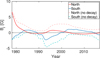 |
Fig. 5. Average field strength above 60° and below −60° latitude from February 1978 (CR 1665) to December 2016 (CR 2184) from simulations that include only every third active region in the southern hemisphere and no active regions in the northern hemisphere with the decay term (solid lines) and without the decay term (dashed lines). |
To assess how long the polar fields would exist without flux emergence in either hemisphere, we ran the simulation using active regions from both hemispheres until June 1984 (CR 1750) and then continued the simulation without any active regions in either hemisphere. In June 1984, the solar cycle 21 was in its declining phase, and polar fields were near their peak intensity. Figure 6 shows the strength of polar fields from this no-activity simulation, as well as from the full-activity simulation, and a full-activity simulation without the decay term. Because it takes several years for flux to travel from the activity belts to the poles, until late 1980s the polar fields in the no-activity simulation remain identical to the polar fields of the full-activity simulation even without flux emergence. They start to significantly differ from the reference simulation around 1989, when the first large flux surges of cycle 22 reach high latitudes and reduce (and eventually reverse) the field of the full-activity simulation. After one sunspot cycle of no activity, in mid-1990s, the field strength is only about 0.5G and after two cycles, around 2005, the field strength is below 0.1G. Naturally, no polarity reversals are observed after mid-1980s in no activity simulations after flux generation was canceled.
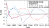 |
Fig. 6. Average field strength above 60° and below −60° latitude from February 1978 (CR 1665) to December 2016 (CR 2184) in a full-activity simulation (dashed lines), in a no-activity simulation (solid lines) that does not include emerging flux after CR 1750, and in a no-activity simulation without the decay term (dotted lines). |
The polar fields of the no-activity simulation without the decay term are included in Fig. 6 to demonstrate the necessity of the decay term. Without any flux emerging the model does not include a process that could eliminate the prior strong polar fields. This unphysical situation would then remain indefinitely. While these results strongly support the need for a decay term in SFT models in order to properly represent the long-term evolution of polar fields in the absence of sufficient emergence of new flux, the exact time scale of such decay requires further investigation.
7. Conclusions
In this paper, we have used an SFT simulation to study how hemispherically asymmetric activity affects the long-term evolution of the photospheric magnetic field and especially the polar areas. Our simulations indicate that polar field reversals can occur in both hemispheres even if sunspot activity is restricted to only one hemisphere. The magnetic flux (mainly of leading polarity) is transported across the solar equator by dissipation (e.g., supergranular diffusion). After the flux crosses the equator, it is also affected by the regular poleward transport via meridional circulation. We find that the overall flux transport (including cross-equatorial dissipation) is sufficiently effective for sunspot activity in one hemisphere only to be able to maintain regular polarity reversals and to reconstruct the polar fields of new polarity in both hemispheres.
In an SFT simulation, the cross-equatorial transport of magnetic flux is driven by supergranular diffusion. In fact, there is observational evidence of such a transport. For example, cross-equatorial flux transport was reported by Cameron et al. (2013), Iijima et al. (2017). Mordvinov et al. (2016) described the evolution of a poleward surge that originated in a small active region of the opposite hemisphere. We find that the fraction of emerging flux transported across the equator is on the order of 1%, but most of this flux diffuses soon after crossing into the northern hemisphere. Only 0.1%–0.2% of the total emerging flux of the active southern hemisphere reaches the northern polar area. The amplitude of the northern polar field is roughly one half to one fourth of the amplitude of the polar field of a regular cycle with full activity in both hemispheres. This is sufficient to produce a regular next cycle in the northern hemisphere, albeit of smaller amplitude.
Limiting sunspot activity to one single hemisphere leads to a significant asynchronicity in the timing of polar field reversals. The reversal of the northern pole delays with respect to the reversal of the active southern hemisphere pole. The time difference between polar field reversals is typically a few (2–4) yr, depending on the level and temporal history of sunspot activity in the active hemisphere. This also leads to a quadrupole Sun where both poles have the same polarity for a long period of time.
The late polarity reversal in the northern hemisphere is due to the flux having to travel a longer-than-usual distance from the southern hemisphere. Moreover, the cross-equatorial transport is rather slow and very irregular. The polarity and speed of the cross-equatorial transport depend on flux emergence in the southern hemisphere. The flow is strongest after solar maxima in the declining phase of the cycle, when active regions emerge near the equator. The northward transport of flux becomes more stable as it reaches higher latitudes. This flux transport makes the polar field change its polarity roughly every 11 yr, thus maintaining the 22-yr magnetic cycle.
Most of the flux crossing the equator is of leading polarity, but some flux of trailing polarity also flows to the northern hemisphere. The ratio of flux of trailing and leading polarities varies from cycle to cycle, and is by far largest during cycle 23. Trailing polarity flux can cross the equator more easily if there is no activity in the opposite hemisphere. Instead, during a normal cycle with activity in both hemispheres, the flow of trailing polarity has a high probability of colliding with the same polarity leading flux on the other side of the equator. The enhanced cross-equatorial transport of trailing flux during cycle 23 weakens both polar fields in the south-activity simulation compared to cycles 21 and 22.
Reducing the amount of emerging flux by factor of three in the south-activity simulation does not stop the polarity reversals in the northern hemisphere. The polar fields become weaker, but polarity keeps on reversing even in the northern hemisphere. Because of the fairly rapid flux decay the earlier, more active sunspot cycles do not prevent the polarity from reversing during the subsequent, weaker cycles. Thus the Sun is able to transition from an active phase to an inactive phase very quickly, still preserving the evolution of the magnetic Hale cycle.
If there is no emerging flux in either hemisphere, both polar fields disappear almost completely within two solar cycles. We have previously shown that it takes about one solar cycle for normal polar fields to develop if the simulation is started without them (Virtanen et al. 2017). These results suggest that if there was a long period, like a grand minimum, without activity in either hemisphere, the polar fields would decay without polarity reversal, and it would take one normal cycle for them to get regenerated. However, a few years without activity, like in a normal sunspot minimum, is not enough for the polar fields to decay away.
Sunspot observations show that during the Maunder minimum sunspot activity was concentrated to the southern hemisphere, with almost no sunspots appearing in the northern hemisphere (Ribes & Nesme-Ribes 1993). Our simulations show that highly asymmetric activity concentrated in one active hemisphere can maintain a weak polar field in the inactive hemisphere. The polar field of the active hemisphere is not significantly affected by the sunspot inactivity of the other hemisphere. However, the delayed polarity reversals in the lower-activity hemisphere lead to quadrupole Sun during several years which may affect how the cycle is observed in the heliosphere.
Acknowledgments
We acknowledge the financial support by the Academy of Finland to the ReSoLVE Centre of Excellence (project No. 272157). The National Solar Observatory (NSO) is operated by the Association of Universities for Research in Astronomy, AURA Inc under cooperative agreement with the National Science Foundation (NSF). The data used in this work were produced in the framework of the NSO synoptic program (512-channel magnetograph, SPMG and SOLIS). This work was partially supported by the International Space Science Institute (Bern, Switzerland) via International Team 420 on Reconstructing Solar and Heliospheric Magnetic Field Evolution over the Past Century.
References
- Babcock, H. W. 1961, ApJ, 133, 572 [Google Scholar]
- Baumann, I., Schmitt, D., Schüssler, M., & Solanki, S. K. 2004, A&A, 426, 1075 [NASA ADS] [CrossRef] [EDP Sciences] [Google Scholar]
- Baumann, I., Schmitt, D., & Schüssler, M. 2006, A&A, 446, 307 [NASA ADS] [CrossRef] [EDP Sciences] [Google Scholar]
- Cameron, R. H., Dasi-Espuig, M., Jiang, J., et al. 2013, A&A, 557, A141 [NASA ADS] [CrossRef] [EDP Sciences] [Google Scholar]
- Hathaway, D. H., & Upton, L. 2014, J. Geophys. Res. (Space Phys.), 119, 3316 [Google Scholar]
- Hathaway, D. H., & Upton, L. A. 2016, J. Geophys. Res. (Space Phys.), 121, 10 [Google Scholar]
- Iijima, H., Hotta, H., Imada, S., Kusano, K., & Shiota, D. 2017, A&A, 607, L2 [NASA ADS] [CrossRef] [EDP Sciences] [Google Scholar]
- Jiang, J., Cameron, R., Schmitt, D., & Schüssler, M. 2010, ApJ, 709, 301 [NASA ADS] [CrossRef] [Google Scholar]
- Jiang, J., Cameron, R. H., Schmitt, D., & Schüssler, M. 2011, A&A, 528, A82 [NASA ADS] [CrossRef] [EDP Sciences] [Google Scholar]
- Jiang, J., Hathaway, D. H., Cameron, R. H., et al. 2014, Space Sci. Rev., 186, 491 [Google Scholar]
- Jones, H. P., Duvall, Jr., T. L., Harvey, J. W., et al. 1992, Solar Phys., 139, 211 [NASA ADS] [CrossRef] [Google Scholar]
- Keller, C. U., Harvey, J. W., & Giampapa, M. S. 2003, in Innovative Telescopes and Instrumentation for Solar Astrophysics, eds. S. L. Keil, & S. V. Avakyan, Proceedings of SPIE, 4853, 194 [NASA ADS] [CrossRef] [Google Scholar]
- Lean, J. L., Wang, Y. M., & Sheeley, N. R. 2002, Geophys. Res. Lett., 29, 77 [CrossRef] [Google Scholar]
- Leighton, R. B. 1969, ApJ, 156, 1 [Google Scholar]
- Lemerle, A., Charbonneau, P., & Carignan-Dugas, A. 2015, ApJ, 810, 78 [NASA ADS] [CrossRef] [Google Scholar]
- Livingston, W. C., Harvey, J., Slaughter, C., & Trumbo, D. 1976, Appl. Opt., 15, 40 [NASA ADS] [CrossRef] [Google Scholar]
- Mordvinov, A., Pevtsov, A., Bertello, L., & Petri, G. 2016, Solar-Terrestrial Physics (Solnechno-zemnaya fizika), 2, 3 [Google Scholar]
- Ohl, A. I. 1966, Solnechnye Dannye, Bulletin of the Academy of USSR, 12, 84 [Google Scholar]
- Petrovay, K. 2010, Liv. Rev. Sol. Phys., 7, 6 [Google Scholar]
- Pietarila, A., Bertello, L., Harvey, J. W., & Pevtsov, A. A. 2013, Sol. Phys., 282, 91 [NASA ADS] [CrossRef] [Google Scholar]
- Ribes, J. C., & Nesme-Ribes, E. 1993, A&A, 276, 549 [NASA ADS] [Google Scholar]
- Schatten, K. H., Scherrer, P. H., Svalgaard, L., & Wilcox, J. M. 1978, Geophys. Res. Lett., 5, 411 [NASA ADS] [CrossRef] [Google Scholar]
- Schrijver, C. J., De Rosa, M. L., & Title, A. M. 2002, ApJ, 577, 1006 [NASA ADS] [CrossRef] [Google Scholar]
- Schüssler, M. & Baumann, I. 2006, A&A, 459, 945 [NASA ADS] [CrossRef] [EDP Sciences] [Google Scholar]
- Sheeley, Jr., N. R., DeVore, C. R., & Boris, J. P. 1985, Sol. Phys., 98, 219 [NASA ADS] [CrossRef] [Google Scholar]
- SILSO World Data Center. 1978–2016, International Sunspot Number Monthly Bulletin and online catalogue [Google Scholar]
- Upton, L., & Hathaway, D. H. 2014, ApJ, 792, 142 [NASA ADS] [CrossRef] [Google Scholar]
- Virtanen, I., & Mursula, K. 2016, A&A, 591, A78 [NASA ADS] [CrossRef] [EDP Sciences] [Google Scholar]
- Virtanen, I. O. I., Virtanen, I. I., Pevtsov, A. A., Yeates, A., & Mursula, K. 2017, A&A, 604, A8 [NASA ADS] [CrossRef] [EDP Sciences] [Google Scholar]
- Whitbread, T., Yeates, A. R., Muñoz-Jaramillo, A., & Petrie, G. J. D. 2017, A&A, 607, A76 [NASA ADS] [CrossRef] [EDP Sciences] [Google Scholar]
- Worden, J., & Harvey, J. 2000, Sol. Phys., 195, 247 [Google Scholar]
- Yeates, A. R. 2014, Sol. Phys., 289, 631 [NASA ADS] [CrossRef] [Google Scholar]
- Yeates, A. R., Baker, D., & van Driel-Gesztelyi, L. 2015, Sol. Phys., 290, 3189 [NASA ADS] [CrossRef] [Google Scholar]
All Tables
Fraction of emerging flux transported across the equator, 30° latitude, and 60° latitude.
All Figures
|
Fig. 1. Super-synoptic map of the KP and SOLIS photospheric magnetic field observations from January 1978 (CR 1664) to December 2016 (CR 2184). Yellow and blue colors correspond to positive and negative polarity. White vertical lines are periods with no observations. |
| In the text | |
|
Fig. 2. Super-synoptic maps of the photospheric magnetic field from February 1978 (CR 1665) to December 2016 (CR 2184) from simulations using active regions in both hemispheres with the decay term (top panel), in both hemispheres but without the decay term (second panel from the top), only in the southern hemisphere (third panel from the top), and only in the southern hemisphere but without the decay term (bottom panel). |
| In the text | |
|
Fig. 3. Average field strength above 60° and below −60° latitude from the simulations shown in Fig. 2. |
| In the text | |
|
Fig. 4. Amount of flux transported northward by supergranular diffusion at the equator (top panel), and by diffusion and meridional circulation at 30° latitude (second panel from the top) and at 60° latitude (third panel from the top). The bottom panel shows the 13-month smoothed monthly sunspot number for reference (SILSO World Data Center 1978–2016). |
| In the text | |
|
Fig. 5. Average field strength above 60° and below −60° latitude from February 1978 (CR 1665) to December 2016 (CR 2184) from simulations that include only every third active region in the southern hemisphere and no active regions in the northern hemisphere with the decay term (solid lines) and without the decay term (dashed lines). |
| In the text | |
|
Fig. 6. Average field strength above 60° and below −60° latitude from February 1978 (CR 1665) to December 2016 (CR 2184) in a full-activity simulation (dashed lines), in a no-activity simulation (solid lines) that does not include emerging flux after CR 1750, and in a no-activity simulation without the decay term (dotted lines). |
| In the text | |
Current usage metrics show cumulative count of Article Views (full-text article views including HTML views, PDF and ePub downloads, according to the available data) and Abstracts Views on Vision4Press platform.
Data correspond to usage on the plateform after 2015. The current usage metrics is available 48-96 hours after online publication and is updated daily on week days.
Initial download of the metrics may take a while.