| Issue |
A&A
Volume 615, July 2018
|
|
|---|---|---|
| Article Number | A163 | |
| Number of page(s) | 10 | |
| Section | Extragalactic astronomy | |
| DOI | https://doi.org/10.1051/0004-6361/201832726 | |
| Published online | 01 August 2018 | |
Multi-wavelength campaign on NCG 7469
IV. The broad-band X-ray spectrum
1
Dipartimento di Matematica e Fisica, Università degli Studi Roma Tre,
via della Vasca Navale 84,
00146
Roma,
Italy
e-mail: This email address is being protected from spambots. You need JavaScript enabled to view it.
2
INAF - IASF Bologna,
via Gobetti 101,
40129
Bologna,
Italy
3
Univ. Grenoble-Alpes, CNRS, IPAG,
38000
Grenoble,
France
4
Department of Physics, Technion,
Haifa
32000,
Israel
5
Department of Physics, Virginia Tech,
Blacksburg,
VA 24061,
USA
6
Department of Astronomy, University of Maryland,
College Park,
USA
7
Mullard Space Science Laboratory, University College London,
Holmbury St. Mary,
Dorking,
Surrey
RH5 6NT,
UK
8
SRON Netherlands Institute for Space Research,
Sorbonnelaan 2,
3584
CA Utrecht,
The Netherlands
9
Nicolaus Copernicus Astronomical Center, Polish Academy of Sciences,
Bartycka 18,
00-716
Warsaw,
Poland
10
Department of Astronomy, University of Geneva,
16 Chemin d’Ecogia,
1290
Versoix,
Switzerland
11
European Space Astronomy Centre, Villanueva de la Cañada,
PO Box 78,
28691
Madrid,
Spain
12
Leiden Observatory, Leiden University,
PO Box 9513,
2300 RA
Leiden,
The Netherlands
13
School of Physics & Astronomy and Wise Observatory, Raymond and Beverly Sackler Faculty of Exact Sciences, Tel-Aviv University,
Tel-Aviv
69978,
Israel
14
Space Telescope Science Institute,
3700 San Martin Drive,
Baltimore,
MD 21218,
USA
15
Max-Planck-Institut für extraterrestrische Physik,
Giessenbachstrasse,
85748
Garching,
Germany
Received:
29
January
2018
Accepted:
19
March
2018
Abstract
We conducted a multi-wavelength 6-month campaign to observe the Seyfert Galaxy NGC 7469, using the space-based observatories HST, Swift, XMM-Newton and NuSTAR. We report the results of the spectral analysis of the seven simultaneous XMM-Newton and NuSTAR observations. The source shows significant flux variability within each observation, but the average flux is less variable among the different pointings of our campaign. Our spectral analysis reveals a prominent narrow neutral Fe Kα emission line in all the spectra and weaker contributions from Fe Kβ, neutral Ni Kα, and ionized iron. We find no evidence for variability or relativistic effects acting on the emission lines, which indicates that they originate from distant material. In the joint analysis of XMM-Newton and NuSTAR data, a constant photon index is found (Γ = 1.78 ± 0.02) together with a high energy cut-off Ecut = 170−40+60 keV. Adopting a self-consistent Comptonization model, these values correspond to an average coronal electron temperature of kT = 45−12+15 keV and, assuming a spherical geometry, an optical depth τ = 2.6 ± 0.9. The reflection component is consistent with being constant and the reflection fraction is in the range R = 0.3−0.6. A prominent soft excess dominates the spectra below 4 keV. This is best fit with a second Comptonization component, arising from a warm corona with an average kT = 0.67 ± 0.03 keV and a corresponding optical depth τ = 9.2 ± 0.2.
Key words: galaxies: active / galaxies: Seyfert / quasars: general / X-rays: galaxies
© ESO 2018
1 Introduction
Active galactic nuclei (AGN) are among the brightest sources in the Universe and they account for a large percentage of the X-ray photons we observe in the sky. It is commonly accepted that AGN are powered by matter accreting onto a supermassive black hole (SMBH). In the innermost region of the host galaxy, a SMBH is surrounded by a disc of spiralling matter that is responsible for its optical-UV emission, while the physical origin of the higher energetic photons still remains elusive. According to the commonly accepted scenario, X-rays are produced in a region close to the central black hole (BH), the so-called hot corona (e.g. Haardt & Maraschi 1991, 1993; Haardt et al. 1994), in which seed optical-UV photons arising from the accreting disc interact with hot thermal electrons through an inverse Compton process. This process reproduces the power law shape we commonly observe in AGN spectra (e.g. Guainazzi et al. 1999; Bianchi et al. 2009; Marinucci et al. 2014). Moreover, a high energy cut-off is observed in different AGN spectra (e.g. Perola et al. 2002; De Rosa et al. 2002; Guainazzi et al. 2010; Brenneman et al. 2014; Marinucci et al. 2014; Lohfink et al. 2015; Ursini et al. 2016; Tortosa et al. 2017, 2018a; Porquet et al. 2018), and this is another signature of the thermal Comptonization acting in the hot corona (Haardt & Maraschi 1991, 1993). Furthermore, the primary continuum emission can be modified by a Compton reflection from the disc, from farther material or by absorption from neutral or from ionized gas.
As an additional hallmark of AGN activity there is continuum variability. Flux variations are indeed observed on several timescales, from hours and days (e.g. Ponti et al. 2012) up to years and decades (e.g. Vagnetti et al. 2011, 2016; Middei et al. 2017). Rapid variability not only is of primary importance to investigate the X-ray emission, but it can be also used to estimate the SMBH mass (e.g. McHardy et al. 2006; Ponti et al. 2012) and as a luminosity distance estimator (La Franca et al. 2014).
Long multi-wavelength monitorings of single nearby AGN produced outstanding results (e.g. Kaastra et al. 2011, and the related series of papers on Mrk 509). The target of our observational campaign is NGC 7469, which is a luminous Seyfert galaxy (Lbol ~ 1045 erg s−1; Behar et al. 2017)at z = 0.016268 (Springob et al. 2005). Using reverberation mapping, Peterson et al. (2014) found that NGC 7469 hosts a BH with a mass of 1.1 ± 0.1 × 10⁷ M⊙ and an Eddington ratio of the order of 0.3. In X-ray wavelengths, this Seyfert Galaxy was first observed by the Uhuru satellite (Forman et al. 1978) in the seventies, and it was subsequently studied by many other observatories that found this source to have a complex X-ray emission. Since the EXOSAT observation, we know that its X-ray spectrum displays an excess in the soft band (Barr 1986). Other authors (Turner et al. 1991; Brandt et al. 1993; Guainazzi et al. 1994; Nandra et al. 1998, 2000; De Rosa et al. 2002) analysed this source using data obtained by Einstein, ROSAT, ASCA, RXTE and BeppoSAX.
NGC 7469 was also studied more recently: Petrucci et al. (2004) investigated the UV/X-ray variability, Scott et al. (2005) analysed its simultaneous X-ray, far-ultraviolet, and near-ultraviolet spectra using Chandra, FUSE and STIS, while Patrick et al. (2011) studied this source taking advantage of Suzaku observations. Previous XMM-Newton data were analysed in Blustin et al. (2003) and De Marco et al. (2009), while some results from the 2015 observational campaign have been presented in Behar et al. (2017) and Peretz et al. (2018).
This paper focuses on the seven simultaneous XMM-Newton and NuSTAR observations of our campaign, and it is organized asfollows. Section 2 presents the NGC 7469 temporal analysis. Section 3 focuses on the data reduction. Sections 4 and 5 report on the spectral analysis. Section 6 contains the discussion of the results, and in Sect. 7 a summary of this work is reported.
2 Observations and data reduction
The spectral analysis presented in this work is based on XMM-Newton (Jansen et al. 2001) and NuSTAR (Harrison et al. 2013) observations of NGC 7469 belonging to the multi-wavelength campaign first described by Behar et al. (2017). The two satellites observed the source simultaneously between June 12 and December 28, 2015. The seven observations are spaced by different time intervals, allowing us to study flux and spectral variations on different timescales, see Table 1.
XMM-Newton data were obtained using the EPIC cameras (Strüder et al. 2001; Turner et al. 2001) in the Small Window operating mode and they were processed taking advantage of the XMM-Newton Science Analysis System1 (SAS, Version 15.0.0). Because of its larger effective area with respect to the two MOS cameras, we only report the results for the PN instrument. We extract spectra from circular regions of 50 arcsec radius for the background, and 40 arcsec radius for the source. These regions are selected by an iterative process that maximizes the signal-to-noise ratio (S/N; Piconcelli et al. 2004). All the spectra were rebinned in order to have at least 30 counts for each bin and not to oversample the spectral resolution by a factor greater than three.
NuSTAR data were reduced taking advantage of the standard pipeline (nupipeline) in the NuSTAR Data Analysis Software (nustardas release: nustardas_14Apr16_v1.6.0, part of the heasoft distribution2), adopting the latest calibration database. The NuSTAR observatory carries in its focal plane two modules, A and B, corresponding to the hard X-ray detectors FPMA and FPMB. Spectra and light curves were extracted for both modules using the standard tool nuproducts. A circular region with radius of ~70 arcsec is used to extract the source counts while the background is obtained from a blank area with the same radius, close to the source. Similar to the XMM-Newton spectra, we binned NuSTAR spectra to have an S/N greater than five in each spectral channel, and to avoid oversampling the instrumental resolution by a factor greater than 2.5. The spectra of the two modules are in good agreement with each other, the cross-normalization constant for FPMB with respect to FPMA in all the fits being unity within 1%. Spectra were analysed with XSPEC 12.9 (Arnaud 1996). All errors reported in the plots account for 1σ uncertainty, while errors in text and tables are quoted at 90% confidence level, unless otherwise stated.
Observation ID, start date, and net exposure time (ks) for each satellite, and for the seven observations analysed in this work.
3 Temporal analysis
We started investigating the NGC 7469 temporal properties computing the light curves for all the observations. We used the standard command epiclccorr for the XMM-Newton data to compute corrected for the background light curves in the 0.5–2 keV and 2–10 keV bands, while, we used the nuproducts pipeline to compute the NuSTAR light curves in the 10–80 keV band. The XMM-Newton and NuSTAR light curves of all the observations of our campaign are shown in Fig. 1. The source shows a remarkable intra-observation flux variability (e.g. up to ~60% in the sixth observation for the XMM-Newton in the 0.5–2 and 2–10 keV bands) and has significant flux variations on timescales of a few ks. On longer timescales, flux variability appears to be less significant. The mean counts for each of the seven observations is observed to be, on average, weakly variable (~15%, ~9%, and few per cent in the 0.5–2, 2–10, and 10–80 keV bands, respectively).
A convenient analysis tool for variability characterization is the so-called normalized excess variance (NXS). The NXS is defined as  , where μ is the unweighted count rate mean within the segment of the light curve, N is the number of the good time bins in that segment, and Xi represents the count rate with
  as associated uncertainty. We computed the
  in the 2–10 keV band for all the observations of our campaign in the 20 ks time bin (see Ponti et al. 2012 for more details), finding an average value
  = 0.0021 ± 0.0005. A tight correlation between the X-ray variability of the source and its BH mass has been found by several authors (e.g. Nandra et al. 1997; Vaughan et al. 2003; McHardy et al. 2006; Ponti et al. 2012). In particular, adopting the relation among
  and MBH in Ponti et al. (2012), we are able to estimate the BH mass MBH = 1.1 ± 0.1 × 10⁷ M⊙ for NGC 7469, in very good agreement with the reverberation mapping estimate by Peterson et al. (2014). The soft X-ray appears to be the most variable band, but hardness ratios do not display a large variation (however significant from a statistical point of view, see Sect. 6) both within and among the observations (~8%), see Fig. 1.
Therefore, we decided to use the average spectra of each observation in the following spectral analysis.
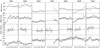 |
Fig. 1 Light curves corresponding to the seven simultaneous observations performed by XMM-Newton and NuSTAR for NGC 7469, in three different energy bands: 0.5–2 keV (first row), 2.0–10 keV (second row), and 10–80 keV (third row). The fourth row shows the ratio between the soft 0.5–2 keV and hard 2.0–10 keV light curves. The axis units are sec and counts for the x-axis and y-axis, respectively.The solid line overlapping all the light curves in each sub-panel represents the average of the counts for the specific light curve. |
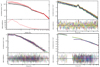 |
Fig. 2 Top left panel: seven XMM-Newton spectra shown in red; the best-fit model to the data above 4 keV shown in black. Bottom panel: the residuals of the seven spectra that are grouped using in Xspec the command ‘setplot group’. A secondary component clearly extends up to 4 keV. Top right panel: best fit to the seven XMM-Newton data and corresponding residuals shown with the basic model (i.e. zashift×(pexrav+zgauss+zgauss)), to which we added other Gaussian lines when weaker emission lines were found in the observation. Bottom left panel: best fit for all NuSTAR spectra above 4 keV is shown; top subpanel shows the bestfit obtained adopting the model that employs xillver (see Sect. 4.2), while the bottom subpanel refers to the corresponding residuals. In the last panel, the best fit (χ2 = 3041 for 2765 d.o.f.) for the NGC 7469 XMM-Newton and NuSTAR spectra; see Sect. 5 for the model details. |
4 Spectral analysis: data above 4 keV
4.1 XMM-Newton: iron line energy band
We start our spectral analysis adopting a simple power law model for all our XMM-Newton data. This crude fit leaves strong residuals in the soft X-rays. This soft excess extends up to 4 keV and is shown in the top left panel of Fig. 2; this value is obtained by fitting the data above 4 keV and then plotting the best-fit model with the whole spectrum, i.e. extending the model into the soft X-ray band. Therefore, as a first step for our analysis, we decided to characterize the limited energy band 4–10 keV. The residuals in this energy band are dominated by strong emission features, readily identified with the Kα lines from neutral and H-like iron, and the possible presence of weaker contributions from neutral Nickel, Fe Kβ, and ionized iron (see Fig. 3).
We therefore adopted the following model to fit the 4–10 keV spectra: zashift ×(pexrav+zgauss+zgauss). The pexrav code (Magdziarz & Zdziarski 1995) is adopted to model the primary emission and any reflected component likely associated with the fluorescent emission line from neutral iron model by the first Gaussian line, while the second Gaussian line accounts for the Fe XXVI Lyα at 6.966 keV. The zashift component is used to correct the well-known XMM-Newton calibration issue affecting the EPIC pn (a detailed discussion on this topic can be found in Cappi et al. 2016). Within this paper, a zashift correction of about − 8 × 10⁻³ (corresponding to ~ 50 eV at 6.4 keV), will always be applied for all the XMM-Newton spectra. To model the data, we let free to vary among the observations the normalizations of both the Fe Kα and the Fe XXVI Lyα lines, the reflection parameter and the photon index in pexrav, and its normalization. The iron abundance is also free to vary but tied among the different observations. This simple model leads us to a very good best fit in the 4–10 keV band (χ2 = 586 for 567 d.o.f.); see top right side panel of Fig. 2.
The Fe Kα and Fe XXVI Lyα lines are both statistically significant (>99.9 per cent according to the F-test), and have a constant flux (3σ level) during the seven observations of our campaign with average values of 3 × 10⁻⁵ and 4 × 10⁻⁶ ph cm−2 s−1, respectively, corresponding to equivalent widths of ~90 and ~20 eV (see Fig. 4 for the Fe Kα line); however, De Marco et al. (2009) analysing previous XMM-Newton data found possible hints of variability in the Fe XXVI Lyα component. We found both the Fe Kα and Fe XXVI Lyα lines are narrow and their intrinsic line width is consistent with zero in all the observations. In particular, the line profiles do not show any evidence for the relativistic effects (see Fig. 3) expected to occur in the innermost regions of the accretion disc.
The residuals in Fig. 3 suggest the presence of the Fe XXV Heα, Fe Kβ, and the Ni Kα emission lines expected at 6.64–6.7, 7.06 and 7.47 keV, respectively, so we tried to fit these lines adding three further Gaussian lines to our best-fit model. However, the inclusion of these lines does not improve the χ2 of the fit significantly. In fact, these three lines are very weak: the Fe Kβ flux is only an upper limit in all the spectra, the nickel line is a detection only in two observations with an average flux of ~ 4.6 × 10⁻⁶ ph cm−2 s−1, and Fe XXV Heα is detected just in three observations with an average flux ~ 4.0 × 10⁻⁶ ph cm−2. Indeed, none of these lines is more significant than 98 per cent, according to the F-test. The best-fit normalizations, or their upper limits, are reported in Table 2 for all the emission lines discussed in this section.
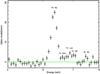 |
Fig. 3 Residuals (in the observer frame) to a simple power law fit to the XMM-Newton spectra in the energy range 5–8 keV. Emission lines are clearly present. The residuals of the seven spectra are grouped for plotting purposes. |
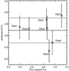 |
Fig. 4 Fe Kα line flux vs. 2–10 continuum flux for the seven XMM-Newton observations. The average line flux is shown together with the standard deviation (dashed lines). |
Best-fit normalizations for the emission lines observed in the XMM-Newton observations.
4.2 NuSTAR: the 4–80 keV spectra
Our preliminary analysis on the 4–10 keV XMM-Newton data shows a non-variable and narrow neutral iron line, likely produced by Compton-thick gas far from the central SMBH. For the NuSTAR data we adopted the self-consistent model xillver (García & Kallman 2010; García et al. 2013) to fit both the neutral iron line and the associated reflection continuum; we use xillver with its ionization parameter fixed to zero. A Gaussian emission line is included to model the observed emission line at 6.966 keV and a second Gaussian line is used for the Fe XXV Heα lines. Strong soft excess features also appear in NuSTAR spectra; thus, similar to what we already performed for XMM-Newton, we preliminary cut NuSTAR spectra below 4 keV. The reflection fraction, the high energy cut-off, normalizations, and the inter-calibration constant are free to vary, while the iron abundance is free to vary but tied among the observations. Following this approach, we obtained the best fit to the data (χ2 = 1762 for 1665 d.o.f.), and this best fit is plotted in the bottom left panel of Fig. 2. The values of the best-fit parameters are reported in Table 3.
This best-fit model requires a super-solar iron abundance AFe= 2.8 ± 0.6. The photon index is consistent with being constant between the observations and has average value of 1.78 ± 0.02 (see Fig. 5, top left panel, showing contour plots). A high energy cut-off is well constrained only in two observations, with values around 150 keV, and there are some indications of variability up to higher values in other observations (see same panel in Fig. 5). However, fitting the NuSTAR spectra tying the high energy cut-off among the seven observations yields a value of  keV with a χ2 = 1775 for 1671 d.o.f. very similar to the previousone in which the high energy cut-off was untied. Some hints of variability are also found for the reflection fraction in the range 0.3–0.6 (see Fig. 5, top right-hand panel, showing contour plots). The flux of the reflection component is consistent with being constant when the primary continuum varies, which is in agreement with an origin from distant matter; we obtained larger reflection components for lower flux states.
Although the iron Kα line does not present any broadening of its profile, we tested for the presence of a relativistic reflection component. Therefore, we added a further reflection component to the best-fit model, accounting for the relativistic effects arising in matter in the innermost regions of the accretion disc. We used relxill (e.g. García et al. 2014; Dauser et al. 2016). The photon index and the high energy cut-off are tied between relxill and xillver, while the relxill ionization parameter ξ and its normalization are free to vary in all the observations. No significant improvement in terms of χ2 ∕d.o.f. is found: Δχ2 = 30 for 18 d.o.f.less, corresponding to 80% confidence level according to F-test. No relativistic reflection is required by the NuSTAR data: indeed, in all but three of the observations, the normalization of relxill is consistent with zero.
According to the standard scenario, hard X-rays are produced by Comptonization, thus as a further investigation, we decided to model the NuSTAR spectra using a self-consistent Comptonization model. In our model we substitute xillver with xillvercp (García et al. 2014; Dauser et al. 2016). This different code accounts for the primary emission produced by nthcomp (Zdziarski et al. 1996) and a non-relativistic reflection. The parameters of this new model are treated as in the previous fit and the hot corona electron temperature is free to vary. The best fit obtained (χ2 = 1768 for 1658 d.o.f.) adopting xillvercp shows larger values for the photon index with respect to the previous best-fit model with xillver (on average 0.08). On the other hand, the parameters of the reflection component are in agreement with the values previously quoted. The best-fit values for the parameters of this fit are shown in Table 4.
In the bottom left panel of Fig. 5, the contour plots for the photon index and hot electron temperature are reported. Weak variations in the photon index are observed, while the electron temperature has a more constant behaviour. To test the variability of the hot electron temperature, similar to what we already performed for the high energy cut-off, we fit the NuSTAR spectra tying the electron temperature among the observations of this campaign. This yielded a measure of  keV corresponding to a best fit (χ2 = 1773 for 1664 d.o.f.) very similar to the previous value.
Values from the best-fit model for all the NuSTAR spectra analysed in the 4–78 keV band using the best-fit model xillver+zgauss+zgauss (χ2 = 1762 for 1665 d.o.f.).
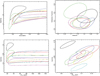 |
Fig. 5 Contours for the high energy cut-off and photon index for all the NuSTAR observations in the top left panel. These contours account for the data analysed with xillver and above 4 keV. The best-fit parameters are shown in Table 3. Top right plot:best-fit values for the reflection fraction as a function of the photon index for the various observations. The contours are computed on the NuSTAR data above 4 keV adopting the model with xillver. Bottom left panel: contour plots for the photon index and hot electron temperature computed on the NuSTAR data above 4 keV with xillvercp. Last panel: contour plots for the warm corona parameters for all the observations of our campaign. |
Values and errors for the best-fit parameters of all the NuSTAR spectra analysed in the 4–78 keV band adopting xillvercp.
5 Spectral analysis: 0.5–80 keV band
As shown inSect. 4.1 (see also Fig. 2, top left hand panel) the data below 4 keV are characterized by a strong soft excess. In order to properly model the continuum emission associated with this excess, we first characterize any discrete emitting and absorbing feature expected in the 0.5–4 keV band. On one side, these are features that can be directly attributed to the detector systematic calibration uncertainties, i.e. issues on itsquantum efficiency at the Si K-edge (1.84 keV), and on the mirrors effective area at the Au M-edge (~ 2.4 keV). To avoid these issues, we ignored the spectral bins in the energy range 1.7–2.6 keV (see e.g. Kaastra et al. 2011; Di Gesu et al. 2015; Ursini et al. 2015; Cappi et al. 2016). We then included all the emission and absorption features (e.g. due to the warm absorbers) derived from the analysis of the XMM-Newton RGS spectra of our campaign by Behar et al. (2017). Since none of these components displayed significant variability during our campaign (Behar et al. 2017; Peretz et al. 2018), we kept all their parameters fixed in our following fits to the values found from the RGS data (see Behar et al. 2017, for a detailed description of all the components). Some line-like features still remained in the pn spectra, and even if very weak, they result significant in terms of χ2, as a consequenceof the high number of counts in the soft band. Two narrow Gaussian lines untied and free to vary among the observations at ~0.75 keV and ~1 keV are enough to correct these residual narrow features (see also e.g. Kaastra et al. 2011; Di Gesu et al. 2015; Ursini et al. 2015; Cappi et al. 2016).
At first, we model the soft X-ray emission with a phenomenological continuum model, such as a power law or a black body. However, in both cases we do not get an acceptable fit, obtaining χ2 = 3542 for 2793 d.o.f. and χ2 = 7430 for 2793 d.o.f., respectively. We then tried to reproduce the soft excess via two self-consistent models: blurred relativistic reflection arising from the innermost regions of the accretion disc, and Comptonization from a warm corona.
There are a number of reasons (e.g. high BH spin and high ionization parameters) that could lead to a weak broad iron line, but still a prominent relativistic reflection continuum, particularly in the soft X-rays. Indeed, Walton et al. (2013), analysing Suzaku data, found a good fit modelling the NGC 7469 soft excess using a relativistic reflection model. Thus, even if our previous analysis failed to find significant signatures from relativistic effects in the hard X-ray band (and, notably, in the iron line profile), we tested for a relativistic origin for the soft excess in this source.
To perform this test, we again added relxill to the model, similar to what previously had been carried out in the NuSTAR data alone, leaving the ionization parameter, coronal emissivity, BH spin, and the normalization free to vary among the observations, while the photon index and high energy cut-off are linked to those in xillver. We get parameters (ξ = 2.4 ± 0.2, i = 45°, emissivity = 4.8 ± 0.3, a > 0.996) consistent with those found by Walton et al. (2013), but our fit is not statistically acceptable (χ2 = 6036 for 2788 d.o.f.). This discrepancy is likely due to the much higher S/N of our data (especially in the soft X-rays) with respect to that used by Walton et al. (2013).
We finally tried nthcomp (Zdziarski et al. 1996; Życki et al. 1999), accounting for a Comptonized continuum from a warm corona, as discussed by Petrucci et al. (2013), Różańska et al. (2015), and Petrucci et al. (2018). For this model we untie and let free to vary the electron temperature and seed photons temperature among the observations. For each observation, all the parameters among XMM-Newton and NuSTAR are tied during the fit, however we need to allow for different values of photon index between XMM-Newton and NuSTAR in every observation. XMM-Newton slopes are harder than the NuSTAR derived slopes and this discrepancy, likely due to residual inter-calibration issues, is, on average, of the order of Δ Γ ~ 0.17 (see e.g. Cappi et al. 2016, and Appendix A for more details). In this paper, we report values of the photon index derived from NuSTAR data.
Following this procedure, we obtained a very good fit to the whole dataset, with χ2 = 3041 for 2765 d.o.f. (see Fig. 2, bottom right-hand side panel). The parameters of the hard X-ray components are fully compatible with those obtained from the fit of the data above 4 keV (Sect. 4.2 and Table 2). We report the best fit values for the parameters describing the soft excess in Table 5. Most of the observed variability can be attributed to the nthcomp normalization that varies among all the observations. On the other hand, the electron temperature is found consistent with being constant, while for the photon index marginal variations are observed; see bottom right-hand side panel of Fig. 5. The measured warm corona temperature (kTwc) is found to be, on average, 0.67 ± 0.03 KeV.
The obtained electron temperature can be used to estimate the optical depth τ for the warm corona. Following Beloborodov (1999), and using his Eq. 13 and the average values for the kTwc and Γ reported in Table 5, we estimate the NGC 7469 warm corona τwc to be 9.2 ± 0.2.
Best-fit parameters for the soft excess, where kTwc is the electron temperature of the warm corona.
6 Discussion
6.1 Two-corona scenario
The broad-band X-ray spectrum of NGC 7469 shows the presence of two main components, the primary power law at high energies and a strong soft excess which starts dominating below ~ 4 keV. This is commonly found in Seyfert galaxies (e.g. Piconcelli et al. 2005; Bianchi et al. 2009; Scott et al. 2012).
The high energy X-ray spectrum can be phenomenologically characterized by a cut-off power law with average spectral index Γ =1.78 ± 0.02 and high energy cut-off 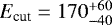 keV. These parameters are consistent with being constant among all the observations, with only some marginal evidence of variability of the cut-off energy. The latter value is compatible within the errors with measures based on Suzaku data (
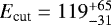 keV; Patrick et al. 2011) and BeppoSAX (Ecut ~ 150 keV; De Rosa et al. 2002). On the other hand, the rapid Γ variability reported by Nandra et al. (2000) could be due to the contamination from the soft excess, which could not be properly modelled in RXTE data. Indeed, it is clear from our monitoring that the soft X-ray energy part of the spectrum varies more than the high energy part, generating variations of the hardness ratio, which could mimic a photon index variability if the two spectral components are not properly modelled separately (see e.g. Figs. 1 and 2, top left panel). However, the rapid Γ variability reported by Nandra et al. (2000) could also be due to a different state of NGC 7469 at the epoch of the IUE/RXTE campaign. In fact, a comparison between our data and those studied by the authors reveals that the source was in a more variable state compared to 2015.
The cut-off power law that reproduces the high energy spectrum of NGC 7469 can be naturally ascribed to Comptonization of the accretion disc photons onto a corona of hot electrons. Adopting a self-consistent Comptonization model, we recovered an average electron temperature of  keV and, under the assumption of a spherical geometry, an optical depth τhc = 2.6 ± 0.9. These values are within ranges generally found in other Seyfert galaxies (e.g. Petrucci et al. 2013, 2018; Tortosa et al. 2018b) and are consistent with being constant among the observations of our monitoring campaign, which is in agreement with what found with phenomenological models. Interestingly, the coronal parameters measured in NGC 7469 lie along the kTe−τ anti-correlation found by Tortosa et al. (2018b) in a sample of Seyfert galaxies observed by NuSTAR. As discussed in their paper, this anti-correlation is suggestive of variations in the heating-cooling ratio of the corona, as a result of different disc-corona geometries and/or intrinsic disc emission. The soft excess cannot be satisfactorily modelled by simple phenomenological models, such as a steep power law or a black body, as often found in large samples of objects and/or low S/N spectra (Bianchi et al. 2009; Matt et al. 2014; Ursini et al. 2015). Moreover, a self-consistent model in terms of blurred relativistic reflection is also statistically unacceptable for reproducing this soft excess.
An additional Comptonized spectral component provides a good representation of the soft excess in this source. Assuming the same seed photons as for the hot corona (i.e. those arising from the accretion disc), the temperature of the electron cloud responsible for the Comptonization of the spectrum is on average kTwc = 0.67 ± 0.03 keV and the optical depth τwc = 9.2 ± 0.2, again with marginal evidence for variability among the observations of our campaign. These values are well in agreement with those found in a sample of Seyfert galaxies, within the framework of the so-called two-corona model (e.g. Petrucci et al. 2013, 2018; Mehdipour et al. 2015; Różańska et al. 2015). According to this model, the soft X-ray emission is produced by Comptonization of the disc photons by a warm optically thick and extended medium (the warm corona), which is different from the compact, optically thin, and hot medium (the hot corona) that is responsible for the high energy emission. The ranges of the coronal values found for the warm corona in Seyfert galaxies (including NGC 7469) are consistent with the warm corona covering a large percentage of a quasi-passive accretion disc, whose intrinsic emission is negligible because most of the accretion power is released in the warm corona itself (Petrucci et al. 2018). It is important to note that this two-corona scenario for NGC 7469 is also consistent with the observed optical-UV emission of this object by HST and Swift UVOT, as quantitatively shown by Mehdipour et al. (2018).
6.2 Reprocessed components
Along with the main continuum components discussed in the previous section, all the XMM-Newton and NuSTAR spectra of our campaign on NGC 7469 are characterized by the presence of a prominent emission line that was readily identified as a neutral Fe Kα fluorescent line. We find that this line is unresolved, has no evidence of any broadening and a flux compatible with being constant among all the observations, and with the past XMM-Newton observation in 2000 (Blustin et al. 2003). As expected if originating in Compton-thick matter, the iron line is associated with a reflection component whose flux is also consistent with being constant among the observations of our campaign. Consequently, its reflection fraction with respect to the primary continuum is slightly variable (R being in the range 0.3−0.6), and higher values are measured when the primary flux is lower. Self-consistent reflection models agree with a scenario in which both the iron lineand reflection component arise from Compton-thick matter far from the accretion disc, as commonly found in the X-ray spectra of Seyfert galaxies (e.g. Bianchi et al. 2009; Cappi et al. 2016; Tortosa et al. 2017).
As already noted, we find no evidence for relativistic effects in the iron line profile of NGC 7469. However, it has to be compared with the rich literature for this source. Guainazzi et al. (1994) found the Fe Kα line to be narrow in a 40 ks ASCA spectrum. In particular, the authors estimated the line-emitting region to be at several tens of Schwarzschild radii from the central engine of the galaxy. This result was confirmed by Nandra et al. (1997) with the same dataset. Subsequently, Blustin et al. (2003) working on XMM-Newton data observed the Fe Kα line to be narrow, and they modelled it with a single narrow Gaussian line. On the other hand, the analysis of BeppoSAX data by De Rosa et al. (2002), pointed to a relativistically broadened component of the line, together with an unresolved core. The presence of a relativistic component was confirmed, albeit marginally, by Suzaku (Patrick et al. 2011; Mantovani et al. 2016).
Although we cannot exclude the presence of a broad component of the iron line in past observations, we may speculate that the narrow core we observe in XMM-Newton data may be contaminated by other emission lines in spectra with lower spectral resolution and/or S/N.Indeed, other emission features are clearly present in the XMM-Newton spectra, as shown in Fig. 3: a strong Fe XXVI Lyα emission line, which was significantly detected in all the observations of our campaign, and weaker emission lines such as Fe XXV Heα, neutral Fe Kβ and Ni Kα, which were not always significant. While the latter two emission lines are expected to accompany the neutral Fe Kα emission, and therefore share the same origin, the other lines must arise in a much more ionized plasma. Such lines are often observed both in Seyfert 1s and in Seyfert 2s and are likely produced in a Compton-thin, photoionized material illuminated by the nuclear continuum (e.g. Bianchi & Matt 2002; Bianchi et al. 2005; Costantini et al. 2010).
7 Conclusions
In this paper we reported the spectral analysis of seven simultaneous NuSTAR and XMM-Newton observations of the Seyfert Galaxy NGC 7469 performed from June 2015 to December 2015 in the context of a multi-wavelength campaign. In the following, we summarize the results of our analysis:
-
NGC 7469 displayed a significant flux variability during this observational campaign with intra-observation variability at a timescales of few ks. We quantified this variability using the normalized excess variance estimator (e.g. Ponti et al. 2012)
 ± 0.0005; this also allowed us to estimate the BH mass to be MBH = 1.1 ± 0.1 × 10⁷
M⊙, which is in agreement with the measure based on reverberation mapping (Peterson et al. 2014).
± 0.0005; this also allowed us to estimate the BH mass to be MBH = 1.1 ± 0.1 × 10⁷
M⊙, which is in agreement with the measure based on reverberation mapping (Peterson et al. 2014). -
The high energy spectrum can be phenomenologically characterized by a cut-off power law with average spectral index Γ = 1.78 ± 0.02 and high energy cut-off Ecut =
 keV. These parameters are consistent with being constant among all the observations, with only some marginal evidence of variability of the cut-off energy. Using a realistic Comptonization model, the derived coronal parameters are
 keV and τhc = 2.6 ± 0.9 for a spherical geometry.
 -
A strong soft excess is observed in all the observations, extending up to 4 keV. The best description for this component is through another Comptonized spectrum that is produced by a warm corona with kTwc = 0.67 ± 0.03 keV and τwc = 9.2 ± 0.2, again with only marginal evidence for variability among the observations of our campaign. Indeed, most of the observed variability of the soft X-ray data may be simply ascribed to variations of the normalization of this component. The overall scenario is consistent with the so-called two-corona model (e.g. Petrucci et al. 2013, 2018; Różańska et al. 2015), where most of the accretion power is released in a warm optically thick and extended medium instead of the accretion disc.
-
A neutral Fe Kα emission line is present in all the observations. The line is found to be narrow, with no indications for relativistic broadening, and consistent with being constant. An accompanying Compton reflection component is also found to be constant among the observations, which is in agreement with a scenario in which both components arise from Compton-thick matter located far away from the central BH. Weak neutral Fe Kβ and Ni Kα emissionlines, which were only detected in some observations, have the same origin.
-
A Fe XXVI Lyα emission line is significantly detected in all the observations of this campaign, and is likely to arise in a photoionized material illuminated by the central continuum, together with a weaker Fe XXV Heα emissionline.
Acknowledgements
We thank the referee for helping us improve the quality of this paper. This work has made use of data from the NuSTAR mission, a project led by the California Institute of Technology, managed by the Jet Propulsion Laboratory, and funded by the National Aeronautics and Space Administration. We thank the NuSTAR Operations, Software and Calibration teams for support with the execution and analysis of these observations. This research has made use of the nustardas jointly developed by the ASI Science Data Center (ASDC, Italy) and the California Institute of Technology (USA). The work is also based on observations obtained with XMM-Newton, an ESA science mission with instruments and contributions directly funded by ESA Member States and the USA (NASA). RM and SB acknowledge financial support from the European Union Seventh Framework Programme (FP7/2007-2013) under grant agreement no. 312789. SB acknowledges financial support from the Italian Space Agency under grant ASI-INAF I/037/12/0. POP acknowledges financial support from the CNES french agency and the CNRS PNHE. GP acknowledges support by the Bundesministerium fü r Wirtschaft und Technologie/Deutsches Zentrum für Luftund Raumfahrt (BMWI/DLR, FKZ 50 OR 1408) and the Max Planck Society. SRON is supported financially by NWO, the Netherlands Organization for Scientific Research.BDM acknowledges support from the Polish National Science Center grant Polonez 2016/21/P/ST9/04025. The research at the Technion is supported by the I-CORE programme of the Planning and Budgeting Committee (grant number 1937/12). EB acknowledges funding from the European Union’s Horizon 2020 research and innovation programme under the Marie Sklodowska–Curie grant agreement no. 655324. M.C. acknowledges financial contribution from the agreement ASI-INAF n.2017-14-H.O
Appendix A Γ discrepancy between XMM-Newton and NuSTAR
We reported in our analysis that our simultaneous XMM-Newton and NuSTAR data yielded photon indexes differing on average of ~ 0.17. In this appendix, we report our investigations concerning a plausible origin for this issue.
-
Different energy band: the energetic range of NuSTAR is different with respect to that of XMM-Newton, thus we performed a simple analysis on the same observational band for both the satellites. For the whole sample of observations, we try to fit the spectra with a simple power law model in the common energy band 4–10 keV. The measurements for the photon indexes we obtained were still discrepant of the same amount.
-
Pile-up: our XMM-Newton spectra could, at least marginally, suffer from pile-up. According to the XMM-Newton hand guide3, pile-up can affect pn observations performed in Small Window mode, when a total count rate of ~25 c/s is exceeded. Therefore, at least the first and second XMM-Newton observations could suffer from pile-up problems.
-
We thus tried to extract the spectra from source annular regions, using different values for the annulus inner radius (from 50 up to 200 pixels). However, our tests show that any choice of the inner annular radius improves the ΔΓ discrepancy between the XMM-Newton and NuSTAR spectra.
-
Intrinsicvariability: XMM-Newton observations are longer with respect to those performed by NuSTAR, thus the difference in the two Γ could bedue to the not truly simultaneity of the observations. To verify this hypothesis we extracted XMM-Newton spectra exactly in the same temporal range of those obtained using NuSTAR4. As in theprevious cases, analysing these truly simultaneous spectra does not affect the ΔΓ discrepancy.
We therefore conclude that the most likely origin for the spectral index discrepancy has to be found in residual inter-calibration issues between XMM-Newton and NuSTAR5, whose significativity may vary from observation to observation, and whose impact on the analysis is larger for high S/N data. We estimate that the results in this paper are not qualitatively affected by this issue, but a systematic uncertainty in the reported best-fit parameters should be taken into account.
References
- Arnaud, K. A. 1996, in Astronomical Data Analysis Software and Systems V, eds. G. H. Jacoby, & J. Barnes, ASP Conf. Ser., 101, 17 [NASA ADS] [Google Scholar]
- Barr, P. 1986, MNRAS, 223, 29 [NASA ADS] [CrossRef] [Google Scholar]
- Behar, E., Peretz, U., Kriss, G. A., et al. 2017, A&A, 601, A17 [NASA ADS] [CrossRef] [EDP Sciences] [Google Scholar]
- Beloborodov, A. M. 1999, in High Energy Processes in Accreting Black Holes, eds. J. Poutanen & R. Svensson, ASP Conf. Ser., 161, 295 [NASA ADS] [Google Scholar]
- Bianchi, S., & Matt, G. 2002, A&A, 387, 76 [NASA ADS] [CrossRef] [EDP Sciences] [Google Scholar]
- Bianchi, S., Matt, G., Nicastro, F., Porquet, D., & Dubau, J. 2005, MNRAS, 357, 599 [NASA ADS] [CrossRef] [Google Scholar]
- Bianchi, S., Guainazzi, M., Matt, G., Fonseca Bonilla, N., & Ponti, G. 2009, A&A, 495, 421 [NASA ADS] [CrossRef] [EDP Sciences] [Google Scholar]
- Blustin, A. J., Branduardi-Raymont, G., Behar, E., et al. 2003, A&A, 403, 481 [NASA ADS] [CrossRef] [EDP Sciences] [Google Scholar]
- Brandt, W. N., Fabian, A. C., Nandra, K., & Tsuruta, S. 1993, MNRAS, 265, 996 [NASA ADS] [CrossRef] [Google Scholar]
- Brenneman, L. W., Madejski, G., Fuerst, F., et al. 2014, ApJ, 788, 61 [NASA ADS] [CrossRef] [Google Scholar]
- Cappi, M., De Marco, B., Ponti, G., et al. 2016, A&A, 592, A27 [NASA ADS] [CrossRef] [EDP Sciences] [Google Scholar]
- Costantini, E., Kaastra, J. S., Korista, K., et al. 2010, A&A, 512, A25 [NASA ADS] [CrossRef] [EDP Sciences] [Google Scholar]
- Dauser, T., García, J., Walton, D. J., et al. 2016, A&A, 590, A76 [NASA ADS] [CrossRef] [EDP Sciences] [Google Scholar]
- De Marco, B., Iwasawa, K., Cappi, M., et al. 2009, A&A, 507, 159 [NASA ADS] [CrossRef] [EDP Sciences] [Google Scholar]
- De Rosa, A., Fabian, A. C., & Piro, L. 2002, MNRAS, 334, L21 [NASA ADS] [CrossRef] [Google Scholar]
- Di Gesu, L., Costantini, E., Ebrero, J., et al. 2015, A&A, 579, A42 [NASA ADS] [CrossRef] [EDP Sciences] [Google Scholar]
- Forman, W., Jones, C., Cominsky, L., et al. 1978, ApJS, 38, 357 [NASA ADS] [CrossRef] [Google Scholar]
- García, J. & Kallman, T. R. 2010, ApJ, 718, 695 [NASA ADS] [CrossRef] [Google Scholar]
- García, J., Dauser, T., Reynolds, C. S., et al. 2013, ApJ, 768, 146 [NASA ADS] [CrossRef] [Google Scholar]
- García, J., Dauser, T., Lohfink, A., et al. 2014, ApJ, 782, 76 [NASA ADS] [CrossRef] [Google Scholar]
- Guainazzi, M., Matsuoka, M., Piro, L., Mihara, T., & Yamauchi, M. 1994, ApJ, 436, L35 [NASA ADS] [CrossRef] [Google Scholar]
- Guainazzi, M., Matt, G., Molendi, S., et al. 1999, A&A, 341, L27 [NASA ADS] [Google Scholar]
- Guainazzi, M., Bianchi, S., Matt, G., et al. 2010, MNRAS, 406, 2013 [NASA ADS] [Google Scholar]
- Haardt, F. & Maraschi, L. 1991, ApJ, 380, L51 [NASA ADS] [CrossRef] [Google Scholar]
- Haardt, F. & Maraschi, L. 1993, ApJ, 413, 507 [NASA ADS] [CrossRef] [MathSciNet] [Google Scholar]
- Haardt, F., Maraschi, L., & Ghisellini, G. 1994, ApJ, 432, L95 [NASA ADS] [CrossRef] [Google Scholar]
- Harrison, F. A., Craig, W. W., Christensen, F. E., et al. 2013, ApJ, 770, 103 [NASA ADS] [CrossRef] [Google Scholar]
- Jansen, F., Lumb, D., Altieri, B., et al. 2001, A&A, 365, L1 [NASA ADS] [CrossRef] [EDP Sciences] [Google Scholar]
- Kaastra, J. S., Petrucci, P.-O., Cappi, M., et al. 2011, A&A, 534, A36 [NASA ADS] [CrossRef] [EDP Sciences] [Google Scholar]
- La Franca, F., Bianchi, S., Ponti, G., Branchini, E., & Matt, G. 2014, ApJ, 787, L12 [NASA ADS] [CrossRef] [Google Scholar]
- Lohfink, A. M., Ogle, P., Tombesi, F., et al. 2015, ApJ, 814, 24 [NASA ADS] [CrossRef] [Google Scholar]
- Magdziarz, P.,& Zdziarski, A. A. 1995, MNRAS, 273, 837 [NASA ADS] [CrossRef] [Google Scholar]
- Mantovani, G., Nandra, K., & Ponti, G. 2016, MNRAS, 458, 4198 [NASA ADS] [CrossRef] [Google Scholar]
- Marinucci, A., Matt, G., Miniutti, G., et al. 2014, ApJ, 787, 83 [NASA ADS] [CrossRef] [Google Scholar]
- Matt, G., Marinucci, A., Guainazzi, M., et al. 2014, MNRAS, 439, 3016 [NASA ADS] [CrossRef] [Google Scholar]
- McHardy, I. M., Koerding, E., Knigge, C., Uttley, P., & Fender, R. P. 2006, Nature, 444, 730 [NASA ADS] [CrossRef] [PubMed] [Google Scholar]
- Mehdipour, M., Kaastra, J. S., Kriss, G. A., et al. 2015, A&A, 575, A22 [NASA ADS] [CrossRef] [EDP Sciences] [Google Scholar]
- Mehdipour, M., Kaastra, J. S., Costantini, E., et al. 2018, A&A, 615, A72 [Google Scholar]
- Middei, R., Vagnetti, F., Bianchi, S., et al. 2017, A&A, 599, A82 [NASA ADS] [CrossRef] [EDP Sciences] [Google Scholar]
- Nandra, K., George, I. M., Mushotzky, R. F., Turner, T. J., & Yaqoob, T. 1997, ApJ, 477, 602 [NASA ADS] [CrossRef] [Google Scholar]
- Nandra, K., Clavel, J., Edelson, R. A., et al. 1998, ApJ, 505, 594 [NASA ADS] [CrossRef] [Google Scholar]
- Nandra, K., Le, T., George, I. M., et al. 2000, ApJ, 544, 734 [NASA ADS] [CrossRef] [Google Scholar]
- Patrick, A. R., Reeves, J. N., Porquet, D., et al. 2011, MNRAS, 411, 2353 [NASA ADS] [CrossRef] [Google Scholar]
- Peretz, U., Behar, E., Kriss, G. A., et al. 2018, A&A, 609, A35 [NASA ADS] [CrossRef] [EDP Sciences] [Google Scholar]
- Perola, G. C., Matt, G., Cappi, M., et al. 2002, A&A, 389, 802 [NASA ADS] [CrossRef] [EDP Sciences] [Google Scholar]
- Peterson, B. M., Grier, C. J., Horne, K., et al. 2014, ApJ, 795, 149 [NASA ADS] [CrossRef] [Google Scholar]
- Petrucci, P. O., Maraschi, L., Haardt, F., & Nandra, K. 2004, A&A, 413, 477 [NASA ADS] [CrossRef] [EDP Sciences] [Google Scholar]
- Petrucci, P.-O., Paltani, S., Malzac, J., et al. 2013, A&A, 549, A73 [NASA ADS] [CrossRef] [EDP Sciences] [Google Scholar]
- Petrucci, P. O., Ursini, F., De Rosa, A., et al. 2018, A&A 611, A59 [NASA ADS] [CrossRef] [EDP Sciences] [Google Scholar]
- Piconcelli, E., Jimenez-Bailón, E., Guainazzi, M., et al. 2004, MNRAS, 351, 161 [NASA ADS] [CrossRef] [Google Scholar]
- Piconcelli, E., Jimenez-Bailón, E., Guainazzi, M., et al. 2005, A&A, 432, 15 [NASA ADS] [CrossRef] [EDP Sciences] [Google Scholar]
- Ponti, G., Papadakis, I., Bianchi, S., et al. 2012, A&A, 542, A83 [NASA ADS] [CrossRef] [EDP Sciences] [Google Scholar]
- Porquet, D., Reeves, J. N., Matt, G., et al. 2018, A&A, 609, A42 [NASA ADS] [CrossRef] [EDP Sciences] [Google Scholar]
- Różańska, A., Malzac, J., Belmont, R., Czerny, B., & Petrucci, P.-O. 2015, A&A, 580, A77 [NASA ADS] [CrossRef] [EDP Sciences] [Google Scholar]
- Scott, J. E., Kriss, G. A., Lee, J. C., et al. 2005, ApJ, 634, 193 [NASA ADS] [CrossRef] [Google Scholar]
- Scott, A. E., Stewart, G. C., & Mateos, S. 2012, MNRAS, 423, 2633 [NASA ADS] [CrossRef] [Google Scholar]
- Springob, C. M., Haynes, M. P., Giovanelli, R., & Kent, B. R. 2005, ApJS, 160, 149 [Google Scholar]
- Strüder, L., Briel, U., Dennerl, K., et al. 2001, A&A, 365, L18 [NASA ADS] [CrossRef] [EDP Sciences] [Google Scholar]
- Tortosa, A., Marinucci, A., Matt, G., et al. 2017, MNRAS, 466, 4193 [NASA ADS] [Google Scholar]
- Tortosa, A., Bianchi, S., Marinucci, A., et al. 2018a, MNRAS, 473, 3104 [NASA ADS] [CrossRef] [MathSciNet] [Google Scholar]
- Tortosa, A., Bianchi, S., Marinucci, A., Matt, G., & Petrucci, P. O. 2018b, A&A, 614, A37 [NASA ADS] [CrossRef] [EDP Sciences] [Google Scholar]
- Turner, T. J., Weaver, K. A., Mushotzky, R. F., Holt, S. S., & Madejski, G. M. 1991, ApJ, 381, 85 [NASA ADS] [CrossRef] [Google Scholar]
- Turner, M. J. L., Abbey, A., Arnaud, M., et al. 2001, A&A, 365, L27 [NASA ADS] [CrossRef] [EDP Sciences] [Google Scholar]
- Ursini, F., Boissay, R., Petrucci, P.-O., et al. 2015, A&A, 577, A38 [NASA ADS] [CrossRef] [EDP Sciences] [Google Scholar]
- Ursini, F., Petrucci, P.-O., Matt, G., et al. 2016, MNRAS, 463, 382 [NASA ADS] [CrossRef] [Google Scholar]
- Vagnetti, F., Turriziani, S., & Trevese, D. 2011, A&A, 536, A84 [NASA ADS] [CrossRef] [EDP Sciences] [Google Scholar]
- Vagnetti, F., Middei, R., Antonucci, M., Paolillo, M., & Serafinelli, R. 2016, A&A, 593, A55 [NASA ADS] [CrossRef] [EDP Sciences] [Google Scholar]
- Vaughan, S., Edelson, R., Warwick, R. S., & Uttley, P. 2003, MNRAS, 345, 1271 [NASA ADS] [CrossRef] [Google Scholar]
- Walton, D. J., Nardini, E., Fabian, A. C., Gallo, L. C., & Reis, R. C. 2013, MNRAS, 428, 2901 [NASA ADS] [CrossRef] [Google Scholar]
- Zdziarski, A. A., Johnson, W. N., & Magdziarz, P. 1996, MNRAS, 283, 193 [NASA ADS] [CrossRef] [Google Scholar]
- Życki, P. T., Done, C., & Smith, D. A. 1999, MNRAS, 309, 561 [NASA ADS] [CrossRef] [Google Scholar]
‘Users Guide to the XMM-Newton Science Analysis System’, Issue 13.0, 2017 (ESA: XMM-Newton SOC).
NuSTARDAS software guide, Perri et al. (2013), https://heasarc.gsfc.nasa.gov/docs/nustar/analysis/ nustar_swguide.pdf
For the fourth observation, the two satellites do not observe NGC 7469 simultaneously so that we cannot perform this test on it.
A new SAS version was released when we were finalizing this paper (SAS version 16.1). We performed several tests to check if this could affect our results, but found that the reported ΔΓ between XMM-Newton and NuSTAR is not significantly improved.
All Tables
Observation ID, start date, and net exposure time (ks) for each satellite, and for the seven observations analysed in this work.
Best-fit normalizations for the emission lines observed in the XMM-Newton observations.
Values from the best-fit model for all the NuSTAR spectra analysed in the 4–78 keV band using the best-fit model xillver+zgauss+zgauss (χ2 = 1762 for 1665 d.o.f.).
Values and errors for the best-fit parameters of all the NuSTAR spectra analysed in the 4–78 keV band adopting xillvercp.
Best-fit parameters for the soft excess, where kTwc is the electron temperature of the warm corona.
All Figures
|
Fig. 1 Light curves corresponding to the seven simultaneous observations performed by XMM-Newton and NuSTAR for NGC 7469, in three different energy bands: 0.5–2 keV (first row), 2.0–10 keV (second row), and 10–80 keV (third row). The fourth row shows the ratio between the soft 0.5–2 keV and hard 2.0–10 keV light curves. The axis units are sec and counts for the x-axis and y-axis, respectively.The solid line overlapping all the light curves in each sub-panel represents the average of the counts for the specific light curve. |
| In the text | |
|
Fig. 2 Top left panel: seven XMM-Newton spectra shown in red; the best-fit model to the data above 4 keV shown in black. Bottom panel: the residuals of the seven spectra that are grouped using in Xspec the command ‘setplot group’. A secondary component clearly extends up to 4 keV. Top right panel: best fit to the seven XMM-Newton data and corresponding residuals shown with the basic model (i.e. zashift×(pexrav+zgauss+zgauss)), to which we added other Gaussian lines when weaker emission lines were found in the observation. Bottom left panel: best fit for all NuSTAR spectra above 4 keV is shown; top subpanel shows the bestfit obtained adopting the model that employs xillver (see Sect. 4.2), while the bottom subpanel refers to the corresponding residuals. In the last panel, the best fit (χ2 = 3041 for 2765 d.o.f.) for the NGC 7469 XMM-Newton and NuSTAR spectra; see Sect. 5 for the model details. |
| In the text | |
|
Fig. 3 Residuals (in the observer frame) to a simple power law fit to the XMM-Newton spectra in the energy range 5–8 keV. Emission lines are clearly present. The residuals of the seven spectra are grouped for plotting purposes. |
| In the text | |
|
Fig. 4 Fe Kα line flux vs. 2–10 continuum flux for the seven XMM-Newton observations. The average line flux is shown together with the standard deviation (dashed lines). |
| In the text | |
|
Fig. 5 Contours for the high energy cut-off and photon index for all the NuSTAR observations in the top left panel. These contours account for the data analysed with xillver and above 4 keV. The best-fit parameters are shown in Table 3. Top right plot:best-fit values for the reflection fraction as a function of the photon index for the various observations. The contours are computed on the NuSTAR data above 4 keV adopting the model with xillver. Bottom left panel: contour plots for the photon index and hot electron temperature computed on the NuSTAR data above 4 keV with xillvercp. Last panel: contour plots for the warm corona parameters for all the observations of our campaign. |
| In the text | |
Current usage metrics show cumulative count of Article Views (full-text article views including HTML views, PDF and ePub downloads, according to the available data) and Abstracts Views on Vision4Press platform.
Data correspond to usage on the plateform after 2015. The current usage metrics is available 48-96 hours after online publication and is updated daily on week days.
Initial download of the metrics may take a while.