| Issue |
A&A
Volume 615, July 2018
|
|
|---|---|---|
| Article Number | A156 | |
| Number of page(s) | 8 | |
| Section | The Sun | |
| DOI | https://doi.org/10.1051/0004-6361/201732396 | |
| Published online | 31 July 2018 | |
Resonant damping of kink oscillations of thin expanding magnetic tubes
1
Solar Physics and Space Plasma Research Centre (SP 2RC), University of Sheffield,
Hicks Building, Hounsfield Road,
Sheffield
S3 7RH, UK
e-mail: This email address is being protected from spambots. You need JavaScript enabled to view it.
2
ITMO University,
Kronverkskii ave 49,
197101
Saint-Petersburg, Russia
3
Space Research Institute (IKI) Russian Academy of Sciences,
Moscow,
Russia
Received:
1
December
2017
Accepted:
20
February
2018
Abstract
We study the resonant damping of kink oscillations of thin expanding magnetic flux tubes. The tube consists of a core region and a thin transitional region at the tube boundary. The resonance occurs in this transitional layer where the oscillation frequency coincides with the local Alfvén frequency. Our investigation is based on the system of equations that we previously derived. This system is not closed because it contains the jumps of the magnetic pressure perturbation and plasma displacement across the transitional layer. We calculate these jumps and thus close the system. We then use it to determine the decrements of oscillation eigenmodes. We introduce the notion of homogeneous stratification. In accordance with this condition the ratio of densities in the tube core and outside the tube does not vary along the tube, while the density in the transitional layer can be factorised and written as a product of two function, one depending on the variable along the tube and the other on the magnetic flux function. Our main result is that, under the condition of homogeneous stratification, the ratio of the decrement to the oscillation frequency is independent of a particular form of the density variation along the tube. This ratio is also the same for all oscillation eigenmodes.
Key words: magnetohydrodynamics (MHD) / plasmas / waves / Sun: oscillations / Sun: corona
© ESO 2018
1 Introduction
Resonant absorption was first studied as a means of heating fusion plasmas (e.g. Tataronis & Grossmann 1973; Grossmann & Tataronis 1973; Chen & Hasegawa 1974a; Hasegawa & Chen 1976). The theory of resonant waves was applied to magnetospheric problems (e.g. Lanzerotti et al. 1973; Southwood 1974; Chen & Hasegawa 1974b,c; Southwood & Hughes 1983; Southwood & Kivelson 1986; Kivelson & Southwood 1986; Inhester 1986; Rickard & Wright 1995; Alan & Wright 1998). Ionson (1978) suggested resonant absorption of magnetohydrodynamic (MHD) waves as a mechanism for heating the solar corona. Since then, resonant absorption has remained a popular mechanism for explaining solar corona heating (e.g. Kuperus et al. 1981; Ionson 1985; Hollweg 1990; see also the review by Arregui 2015).
On 14 July 1998, a transverse oscillation of coronal magnetic loops was first observed by the Transition Region and Coronal Explorer (TRACE) spacecraft. The results of this observation were reported by Aschwanden et al. (1999) and Nakariakov et al. (1999). In particular, it was reported that this oscillation was strongly damped and the damping time was comparable with the oscillation period. It was suggested that this damping is due to resonant absorption. In fact, it was suggested ten years earlier by Hollweg & Yang (1988) that time hypothetically that oscillations of coronal magnetic loops could be efficiently damped by the resonant absorption. Hollweg & Yang (1988) used the planar geometry but then managed to translate their result to the cylindrical geometry and obtained the correct expression for the decrement of kink oscillations of a magnetic flux tube in the thin tube approximation. Goossens et al. (1992) studied the damping of kink oscillations of magnetic flux tubes due to resonant absorption in the general case. Ruderman & Roberts (2002) applied the theory of wave damping due to resonant absorption to the first observation of coronal loop kink oscillations and showed that the observed damping of these oscillations can be used to obtain information about the internal structure of coronal magnetic loops. They modelled a coronal loop as a magnetic tube that consists of an internal core of radius R and a transitional or boundary layer of thickness l between the dense core plasma and the rarefied surrounding plasma. The decrement is proportional to the ratio of the transitional layer thickness and the core radius. Using the data on the oscillation damping reported by Nakariakov et al. (1999), they obtained that l∕R = 0.23. Goossens et al. (2002) used eleven cases of observations of damped kink oscillations of coronal magnetic loops to estimate the ratio of the transitional layer thickness and the core radius. They obtained values of l∕R between 0.16 and 0.49. Since then, observations of damped coronal loop oscillations are routinely used for getting information on the loop internal structure (e.g. Ruderman & Erdélyi 2009; Goossens et al. 2011).
Both Ruderman & Roberts (2002) and Goossens et al. (2002) used the thin tube and thin boundary layer (TTTB) approximation. While the thin tube approximation is definitely applicable to kink oscillations of coronal magnetic loops because the typical ratio of the tube radius to its length is 0.02, the applicability of the thin boundary layer approximation is not obvious, especially when l∕R = 0.49. However, the numerical study using the exact linearised MHD equations by Van Doorsselaere et al. (2004) shows that the thin boundary approximation works very well even for this value of l∕R.
In the first studies of coronal magnetic loop oscillations a very simple model of a homogeneous magnetic cylinder was used (e.g. Ryutov & Ryutova 1976; Edwin & Roberts 1983). Since in this model the tube has a sharp boundary it does not describe resonant absorption. To describe resonant absorption this model was generalised and a transitional layer at the tube boundary was included. Later, more complex and realistic models of coronal loops were developed. For a review of the theory of transverse coronal looposcillations see, for example, Ruderman & Erdélyi (2009). A review of recent advances in the theory of resonant absorption is given by Goossens et al. (2011). In particular, Dymova & Ruderman (2006) studied the resonant damping of kink oscillations of magnetic tubes stratified in the longitudinal direction using the TTTB approximation. The main result that they obtained is the following: if the ratio of densities in the tube core and in the surrounding plasma is constant, and the ratio of density inside the boundary layer and in the tube core does not vary along the tube, then the ratio of the damping time and oscillation period is not affected by the longitudinal stratification.
Although typically the coronal loop expansion is relatively small, the ratio of the loop cross-sectional radii at the apex and at the foot-points can still reach a value of 1.5 (Klimchuk 2000; Watko & Klimchuk 2000). At the same time in the chromosphere the expansion of vertical magnetic flux tubes can reach a value of up to a few hundred (e.g. Tsuneta et al. 2008). Hence, it is important to take the expansion of the magnetic flux tubes into account when studying their kink oscillations. Ruderman et al. (2008) and Verth & Erdélyi (2008) derived the equation describing kink oscillations of an expanding magnetic flux tube. They considered a magnetic flux tube with a sharp boundary, which implies that the equation that they derived does not describe resonant damping. Recently, Ruderman et al. (2017) generalised this derivation to include a siphon flow in the magnetic tube, temporal variation of the plasma parameters related, for example, to cooling, and a transitional layer at the tube boundary.
In this article we use the equation derived by Ruderman et al. (2017) to study the tube expansion effect on the resonant damping of coronal loop kink oscillations. The article is organised as follows. In the next section we describe the equilibrium state and present the governing equations. In Sect. 3 we derive the expressions for the jumps of the magnetic pressure perturbation and the plasma displacement across the transitional layer. In Sect. 4 we calculate the decrement of an oscillation eigenmode. Section 5 contains the summary of the obtained results and our conclusions.
2 Equilibrium state and governing equations
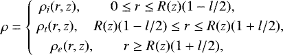
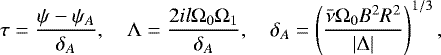
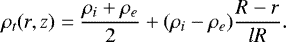
We model a coronal loop as a straight, thin, and expanding magnetic tube with a circular cross section. The tube consists of a core and a transition region where the density decreases from a higher value inside the tube to a lower value representing the surrounding plasma. In cylindrical coordinates r, ϕ, z with the z-axis coinciding with the tube axis, the plasma density is defined by
 (1)
(1)
where R(z) in the radius of the tube cross section, l is a constant determining the thickness of a transitional layer, ρ(r, z) is a continuous function, and ρt(r, z) is a monotonically decreasing function of r. The equilibrium magnetic field is B = (Br(r, z), 0, Bz(r, z)). We assume that the boundaries of the transitional layer are magnetic surfaces. Figure 1 shows a sketch of the equilibrium state of the model proposed. We use the cold plasma approximation and TTTB approximation and assume that  and l ≪ 1, where
  is the tube length. We also assume that the characteristic scale of variation of ρi (r, z), ρe (r, z), and B in the radial direction is
  . On the other hand, the characteristic scale of variation of ρt(r, z) in the radial direction is lR*, where R* is a typical value of R(z). Below we use the notation
  . The tube ends are assumed to be frozen in the dense plasma at
  . When writing down Eq. (1), we assumed that the ratio of the transitional layer thickness to the tube radius is independent of z.
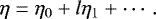
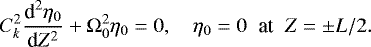
Ruderman et al. (2017) derived the system of two equations that describe kink oscillations of expanding magnetic flux tubes in the presence of siphon flow and the equilibrium quantities varying in time using the cold plasma and TTTB approximation. In the case of static equilibrium, that is when there is no background flow and the equilibrium quantities are time-independent, this system of equations reduces to

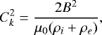
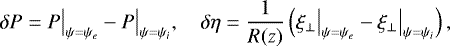
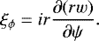
In these equations η = ξ⊥∕R(z), where ξ⊥ is the plasma displacement in the direction perpendicular to B and in the plane ϕ = const, P is the perturbation of the magnetic pressure, μ0 is magnetic permeability of free space,
 (4)
(4)
and δP and δη are the jumps of P and η across the transitional layer defined by
 (5)
(5)
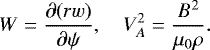
where ψ = ψe and ψ = ψi are the equations of the external and internal boundaries of the transitional layer, respectively. We note that in the thin tube approximation the dependence of B, ρi, and ρe on r is neglected, and these quantities are only considered as functions of z. In Eq. (2) η is calculated in the core of the tube where it is independent of r in the thin tube approximation. It follows from the magnetic flux conservation that B and R are related by
 (6)
(6)
The system of Eqs. (2) and (3) is not closed. To close it, we need to express δP and δη in terms of η. This will be done in the next section.
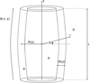 |
Fig. 1 Sketch of equilibrium state. |
3 Derivation of expressions for δP and δη
3.1 Transformation of linearised MHD equations
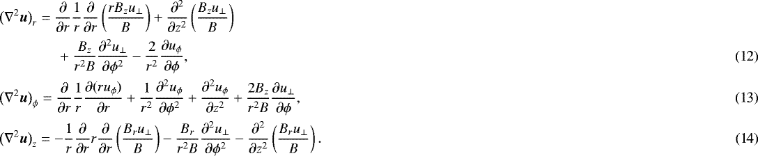
To derive the expressions for δP and δη, we solve the linearised MHD equations using the approximation of cold plasma. To remove the singularity at the Alfvén resonant position, we take the viscosity into account. In the solar corona, viscosity is strongly anisotropic. The full Braginkii’s expression for the viscosity tensor contains five terms (Braginskii 1965). For typical coronal conditions the coefficient at the first term describing the compressional viscosity is at least ten orders of magnitude larger than the coefficients at the fourth and fifth terms describing the shear viscosity. However, in weakly dissipative plasmas like the coronal plasma, the viscosity is only important in the vicinity of the ideal resonant position. In this vicinity only the shear viscosity works (e.g. Ofman et al. 1994; Erdelyi & Goossens 1995). Thus, we can only keep the terms describing shear viscosity. As a result the term describing the viscous force on the right-hand side of the momentum equation is given by ρν∇2 u, where ν is the coefficient of shear viscosity and u = (ur, uϕ, uz) is the velocity. Then the linearised set of MHD equations in the cold plasma approximation is
We now introduce the plasma displacement ξ = (ξr, ξϕ, ξz) related to the velocity by u = ∂ξ∕∂t. Below we use the components of the velocity and plasma displacement that are perpendicular to the equilibrium magnetic field and are in the ϕ = const plane:
 (10)
(10)
We also use the magnetic pressure perturbation P = b ⋅B∕μ0.
Below we need the expression for the viscosity force in terms of ξ⊥ and ξϕ. We use the identity (Korn & Korn 1961)
 (11)
(11)
Using the expressions for the gradient, divergence, and curl in cylindrical coordinates and taking into account that in the cold plasma approximation the velocity perturbation is orthogonal to the equilibrium magnetic field, ξr Br + ξzBz = 0, we obtain
Now we note that in the thin tube approximation  ,
, ![Mathematical equation: $B_z = B[1 + {\cal O}(\epsilon)]$](/articles/aa/full_html/2018/07/aa32396-17/aa32396-17-eq16.png) , and the derivative with respect to z is of the order of ϵ times the derivative either with respect to r or ϕ. In addition, viscosity is only important in the vicinity of the ideal resonant position where the gradients of perturbations strongly dominate the gradients of equilibrium quantities, which implies that the second derivatives with respect to r and ϕ of u⊥ and uϕ strongly dominate all other terms in Eqs. (12)–(14). Then, using the relation between u and ξ, we obtain the approximate expressions:
, and the derivative with respect to z is of the order of ϵ times the derivative either with respect to r or ϕ. In addition, viscosity is only important in the vicinity of the ideal resonant position where the gradients of perturbations strongly dominate the gradients of equilibrium quantities, which implies that the second derivatives with respect to r and ϕ of u⊥ and uϕ strongly dominate all other terms in Eqs. (12)–(14). Then, using the relation between u and ξ, we obtain the approximate expressions:
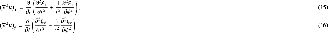
As we have already stated, Ruderman et al. (2017) derived the system of equations describing the kink oscillations in a thin non-stationary expanding tube in the approximation of ideal MHD in the presence of flow (see their Eqs. (29), (34), and (35)). To obtain the system of equations describing the kink oscillations in a thin static expanding tube in the viscous MHD, we take all equilibrium quantities in equations derived by Ruderman et al. (2017) independent of time, set the background velocity equal to zero, eliminate the velocity perturbation, and add the terms describing the viscosity force in the momentum equation. Then we obtain
![Mathematical equation: \begin{align}&P = -\frac1{\mu_0}\left(\frac{B_z}r\frac{\partial(rw)}{\partial r} + \frac{B^2}r\frac{\partial\xi_{\phi}}{\partial\phi} - B_r\frac{\partial w}{\partial z}\right),\\ &\frac{\partial^2 w}{\partial t^2} = \frac{B^2}\rho\left[B_r\frac\partial{\partial z} \left(\frac P{B^2}\right)\right.\!\! - \!\!\left. B_z\frac\partial{\partial r} \left(\frac P{B^2}\right)\right] \nonumber \\ & \quad\quad\quad + \frac B{\mu_0\rho}\left(rB_r\frac\partial{\partial r}\frac1r \right. + \left. B_z\frac\partial{\partial z}\right) \left(\frac{B_r}{rB}\frac{\partial(rw)}{\partial r} \right. \!\! + \!\!\left. \frac{B_z}B\frac{\partial w}{\partial z}\right)\nonumber \\ & \quad\quad\quad+ \nu\frac\partial{\partial t}\left(\frac{\partial^2 w} {\partial r^2} + \frac1{r^2}\frac{\partial^2 w}{\partial\phi^2}\right),\\ &\frac{\partial^2\xi_{\phi}}{\partial t^2} + \frac1{r\rho}\frac{\partial P}{\partial\phi} = \frac1{\mu_0\rho}\left(\frac{B_r}r\frac\partial{\partial r}r + B_z\frac\partial{\partial z}\right) \left(rB_r\frac\partial{\partial r}\left(\frac{\xi_{\phi}}r\right) \right. \nonumber \\ & \quad\quad\quad \quad\quad\quad\quad+ \left. B_z\frac{\partial\xi_{\phi}}{\partial z}\right) + \nu\frac\partial{\partial t}\left(\frac{\partial^2\xi_{\phi}} {\partial r^2} + \frac1{r^2}\frac{\partial^2\xi_{\phi}}{\partial\phi^2}\right),\end{align}](/articles/aa/full_html/2018/07/aa32396-17/aa32396-17-eq18.png)
where w = Bξ⊥. Since ∇ ⋅B = 0, we can express B in terms of the flux function ψ:
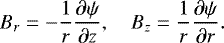 (20)
(20)
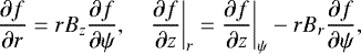
Now similar to Ruderman et al. (2008, 2017) we use ψ as an independent variable instead of r. Then, using the relations
 (21)
(21)
where f is any function, and the subscripts r and ψ indicate that a derivative is taken at constant r and ψ, respectively, and assuming that P, ξ⊥, and ξϕ are proportional to exp(iϕ − iωt), we reduce Eqs. (17)–(19) to
![Mathematical equation: \begin{align}&P = -\frac1{\mu_0}\left(rB^2\frac{\partial w}{\partial\psi} + iB^2\frac{\xi_{\phi}}r - B_r\frac{\partial w}{\partial z} + B_z\frac wr\right),\\ &\omega^2 w = -\frac{rB^2 B_z}{\mu_0\rho}\frac\partial{\partial z} \left(\frac{B_z}{r^2 B^2}\frac{\partial(rw)}{\partial z}\right) - \frac{B^2}\rho\Bigg[B_r\frac\partial{\partial z}\left(\frac P{B^2}\right) \nonumber \\ & \quad\quad\quad- rB^2\frac\partial{\partial\psi}\left(\frac P{B^2}\right)\Bigg] + i\nu\omega \left(r^2 B_z^2\frac{\partial^2 w}{\partial\psi^2} - \frac{w}{r^2}\right),\\ &\omega^2\xi_{\phi} = \frac{iP}{\rho r} - \frac{B_z}{\mu_0\rho r}\frac\partial{\partial z} \left[r^2B_z\frac\partial{\partial z}\left(\frac{\xi_{\phi}}r\right)\right] + i\nu\omega\left(r^2 B_z^2\frac{\partial^2\xi_{\phi}}{\partial\psi^2} - \frac{\xi_{\phi}}{r^2}\right).\end{align}](/articles/aa/full_html/2018/07/aa32396-17/aa32396-17-eq21.png)
We now consider the terms on the right-hand sides (RHS) of Eqs. (23) and (24) that are proportional to ν. The second term in the brackets is of the order of  while the first term is of the order of ξϕ divided by the characteristic spatial scale in the vicinity of the ideal resonant position squared. Since this characteristic spatial scale is much smaller than R*, we can neglect the second term in these brackets. Taking into account that the characteristic scale in the z-direction is
  , we introduce the stretching variable Z = ϵz. We also introduce the scaled frequency Ω = ϵ−1ω, scaled magnetic pressure perturbation Q = ϵ−2P∕B2, and scaled viscosity
  . Then we use the scaled variables to transform Eqs. (22)–(24) and only keep leading terms with respect to ϵ. As a result, we obtain
![Mathematical equation: \begin{align}&\xi_{\phi} = ir^2\frac{\partial w}{\partial\psi} + \frac{iw}B,\\ &\mathrm{\Omega}^2 w = \frac{rB^4}\rho\frac{\partial Q}{\partial\psi} - \frac{rB^3}{\mu_0\rho}\frac\partial{\partial Z} \left(\frac1{r^2 B}\frac{\partial(rw)}{\partial Z}\right) + i\bar\nu\mathrm{\Omega} r^2 B^2\frac{\partial^2 w}{\partial\psi^2},\\ &\mathrm{\Omega}^2\xi_{\phi} = \frac{iB^2 Q}{\rho r} - \frac B{\mu_0\rho r}\frac\partial{\partial Z} \left[r^2B\frac\partial{\partial Z}\left(\frac{\xi_{\phi}}r\right)\right] + i\bar\nu\mathrm{\Omega} r^2 B^2\frac{\partial^2\xi_{\phi}}{\partial\psi^2}.\end{align}](/articles/aa/full_html/2018/07/aa32396-17/aa32396-17-eq25.png)
Substituting r for f in the first relationin Eq. (21), we obtain
 (28)
(28)
where we substituted B for Bz. Using this result we transform Eq. (25) to
 (29)
(29)
3.2 Solution outside the dissipative layer
Since the Alfvén speed in the core region is almost independent of the radial direction, the magnetic field lines frozen in the dense plasma at  oscillate with the same frequency. The same is true for the magnetic field lines outside the magnetic tube. However, there is strong density variation in the transition layer, which implies that there is also strong variation of the Alvén speed. This means that the oscillation frequency of magnetic field lines in the transitional layer depends on ψ. If this oscillation frequency coincides with the frequency of a kink oscillation at a particular magnetic surface, then at this surface there is resonance between the global kink oscillation and the local Alfvén oscillations of magnetic field lines. In a weakly dissipative plasma there are large gradients of perturbations in the vicinity of the resonant surface, and the size of this vicinity is much smaller than lR*. Dissipation is only important in a thin dissipative layer embracing the resonant position. This observation suggests a method of solving problems involving resonant interaction of MHD waves. In this method the wave motion is described by the dissipative MHD equations in the dissipative layer and by the ideal MHD equations on the two sides of this layer. Then the solutions are matched in the two overlap regions.
We calculate δP and δη in the leading order approximation with respect to l. In accordance with this, we substitute Qi for Q in Eq. (27), where Qi is the value of Q calculated at ψ = ψi. Now substituting Eq. (29) in Eq. (27) and taking into account BR2 = const, we obtain
 (30)
(30)
where
 (31)
(31)
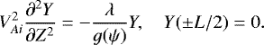
We then consider the Sturm–Liouville problem
 (32)
(32)
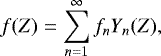
where  . The eigenvalues of this problem are real and constitute a monotonically increasing sequence {λn }, λn →∞ as n →∞ (Coddington & Levinson 1955). It is straightforward to show that all eigenvalues are positive. Any square integrable in the interval [−L∕2, L∕2] function f(z) can be expanded in the generalised Fourier series
 (33)
(33)
where Y n(z) is the eigenfunction corresponding to the eigenvalue λn. Obviously we can choose all eigenfunctions to be real. If f(z) has the continuous second derivative and satisfies the boundary condition f(±L∕2) = 0, then the series in Eq. (33) converges uniformly and can be differentiated twice. The eigenfunctions satisfy the orthogonality condition
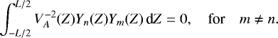 (34)
(34)
Dymova & Ruderman (2006) assumed that the density is factorised and equal to a product of two functions, one depending on r and the other on z. They called this the condition of homogeneous stratification. We similarly assume that the density in the transitional layer can be factorised and expressed as a product of two functions, one depending on z and the other on ψ. Since we neglect the radial dependence of B, this implies that the Alfvén speed can be written as
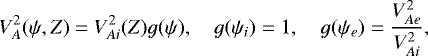 (35)
(35)
where g(ψ) = const for ψ ≤ψi and ψ ≥ψe, g(ψ) is the monotonically increasing function in ψ ∈ (ψi, ψe), V Ai and V Ae are the values of the Alfvén speed at ψ = ψi and ψ = ψe, respectively, and ψ = ψe is the equation of the external boundary of the transitional layer. Then we can rewrite Eq. (32) as
 (36)
(36)
It follows from this equation that
 (37)
(37)
We normalise the eigenfunctions by the condition
 (38)
(38)
Then the Fourier coefficients in Eq. (33) are given by
 (39)
(39)
Below we will see that the ratio of the imaginary and real part of Ω is of the order of l ≪ 1. This enables us to look for Ω in the form Ω0 + lΩ1, where Ω0 and Ω1 are of the same order. In Eq. (30) we keep terms of the order of one and l, while we neglect smaller terms. Hence, we write  . The last term on the left-hand side of Eq. (30) is calculated in the leading order approximation. Hence, we take
  . Since the viscosity is only used to remove the singularity at the ideal resonant surface, we can choose the z-dependence of ν arbitrarily. It is convenient to assume that νB is independent of z. Then it follows from Eq. (6) that the coefficient at the second derivative with respect to ψ in Eq. (30) is independent of Z. Now, substituting the expansions
 (40)
(40)
in Eq. (30), we obtain
![Mathematical equation: \begin{equation*} [\mathrm{\Omega}_0^2 + 2l\mathrm{\Omega}_0\mathrm{\Omega}_1 - \lambda_n(\psi)]W_n - i\bar\nu\mathrm{\Omega}_0 B^2 R^2\frac{\textrm{d}^2 W_n}{\textrm{d}\psi^2} = \mu_0\mathrm{\Phi}_n g(\psi).\end{equation*}](/articles/aa/full_html/2018/07/aa32396-17/aa32396-17-eq43.png) (41)
(41)
The resonant surfaces are defined by the equation
 (42)
(42)
The Alfvén resonance is at any surface defined by this equation. Below we assume that the intervals (λn (ψi), λn(ψe)) do not overlap and  is in one of these intervals. Say it is in the interval where n = N; then there is exactly one value of ψ satisfying Eq. (42) which we denote as ψA. The last term on the left-hand side of Eq. (41) is only important in a dissipative layer embracing the resonant magnetic surface. The thickness of this layer is much smaller than lR*. Outside of this layer we can neglect the last term on the left-hand side of Eq. (41). We also can neglect 2lΩ 0Ω1 in comparison with
  . Then we obtain
 (43)
(43)
Since there is no Alfvén resonance when n≠N, this equation is valid in the whole transition layer when n≠ N. Then using Eq. (31) and substituting R(z) for r yields
 (44)
(44)
We see that there is a non-integrable singularity in the integrals at ψ =ψA when n = N. Substituting R(z) for r in Eq. (26), and using Eqs. (6) and (32), we obtain
_n.\end{equation*}](/articles/aa/full_html/2018/07/aa32396-17/aa32396-17-eq49.png) (45)
(45)
We see that, in contrast to w, Q does not have a singularity at ψ = ψA.
3.3 Connection formulae
As we have seen, the solution to the ideal linear MHD equations has a singularity at ψ = ψA. Near this surface there are large gradients, which implies that the viscosity becomes important in a thin dissipative layer embracing the magnetic surface ψ = ψA. If we are not interested in the motion in the dissipative layer, then all we need from the dissipative solution are the jumps of the total pressure and the normal component of the velocity across this dissipative layer. Sakurai et al. (1991) suggested calling the expressions that give these jumps the connection formulae. They found the solution of the dissipative MHD equations in terms of Bessel functions and obtained the connection formulae for driven problem where the system oscillations are driven by an external source and the system oscillates with the constant amplitude. Later Goossens et al. (1995) obtained the solution in the dissipative layer in terms of so-called F and G functions. Goossens et al. (1992) used the connection formulae to study the damping of magnetic tube kink oscillations. In this study it was assumed that the viscosity is not very weak in the sense that the last term on the left-hand side of Eq. (41) dominates the term proportional to Ω1, so the latter can be neglected. Ruderman et al. (1995) showed that when this is not the case the character of solution in the dissipative layer changes substantially and it becomes strongly oscillatory. Ruderman et al. (1995) studied a planar problem. Tirry & Goossens (1996) generalised this study to the cylindrical geometry. Since the thickness of the dissipative layer is much smaller than that of the transitional layer, the variation of λN (ψ) in the dissipative layer is small and it can be approximated by the first two terms of the Taylor expansion:
 (46)
(46)
Using this equation and introducing the dimensionless quantities τ and Λ defined by
 (47)
(47)
we reduce Eq. (41) with n = N to
![Mathematical equation: \begin{equation*} \frac{\textrm{d}^2 W_N}{\textrm{d}\tau^2} + [i\,\textrm{sign}(\mathrm{\Delta}) + \mathrm{\Lambda}]W_N = \frac{i\mu_0\mathrm{\Phi}_N g(\psi_A)}{\delta_A|\mathrm{\Delta}|}.\end{equation*}](/articles/aa/full_html/2018/07/aa32396-17/aa32396-17-eq52.png) (48)
(48)
This equation can be obtained from Eq. (A1) in Tirry & Goossens (1996) by substituting WN for Ψ, − Λ for Λ, and − μ0ΦN∕δA|Δ| for the right-hand side in the latter. Then we obtain the solution to Eq. (48) making the same substitution in Eq. (A4) in Tirry & Goossens (1996). This yields
 (49)
(49)
where
 (50)
(50)
Now, using Eqs. (31), (49), and (50), the relations η = ξ⊥∕R and w =Bξ⊥, and substituting R for r, we obtain
 (51)
(51)
Integrating this equation yields
 (52)
(52)
where C is an arbitrary constant and
![Mathematical equation: \begin{equation*} G_{\mathrm{\Lambda}}(\tau) = \int_0^{\infty} \frac{e^{-\sigma^3/3}}\sigma \left[\exp(i\sigma\tau\,\textrm{sign}(\mathrm{\Delta}) + \mathrm{\Lambda}\sigma) - 1\right]\textrm{d}\sigma.\end{equation*}](/articles/aa/full_html/2018/07/aa32396-17/aa32396-17-eq57.png) (53)
(53)
The functions FΛ and GΛ were introduced by Goossens et al. (2011). When Λ = 0 they coincide with the F and G functions, respectively. We define the jump of function f(τ) through the dissipative layer as
![Mathematical equation: \begin{equation*} [f(\tau)] = \lim_{\tau \to \infty}[f(\tau) - f(-\tau)].\end{equation*}](/articles/aa/full_html/2018/07/aa32396-17/aa32396-17-eq58.png) (54)
(54)
Then, using the substitution στ = ς, we obtain
![Mathematical equation: \begin{eqnarray*} [G_{\mathrm{\Lambda}}(\tau)] &=& 2i\,\textrm{sign}(\mathrm{\Delta})\lim_{\tau \to \infty}\int_0^{\infty} \exp\left(\frac{\mathrm{\Lambda}\varsigma}\tau - \frac{\varsigma^3}{3\tau^3}\right) \frac{\sin\varsigma}\varsigma\, \textrm{d}\varsigma \nonumber\\ &=& 2i\,\textrm{sign}(\mathrm{\Delta})\int_0^{\infty} \frac{\sin\varsigma}\varsigma\, \textrm{d}\varsigma = \pi i\,\textrm{sign}(\mathrm{\Delta}).\end{eqnarray*}](/articles/aa/full_html/2018/07/aa32396-17/aa32396-17-eq59.png) (55)
(55)
Then using the expansion of η in the Fourier series and Eq. (52), and taking into account that [ηn] = 0 for n≠ N, we finally arrive at
![Mathematical equation: \begin{equation*} [\eta(\tau)] = -\frac{\pi i\mu_0\mathrm{\Phi}_N g(\psi_A)}{|\mathrm{\Delta}|BR^2}\,Y_N(Z).\end{equation*}](/articles/aa/full_html/2018/07/aa32396-17/aa32396-17-eq60.png) (56)
(56)
It follows from Eq. (45) that [Q] = 0.
3.4 Matching solutions
To calculate δη and δP, we need to match the internal solution, which is the solution in the dissipative layer, and the external solution, which is the solution outside the dissipative layer, in two overlap regions at the left and right of the dissipative layer. In these overlap regions both solutions are valid. In accordance with the method of matched asymptotic expansions (e.g. Bender & Orszag 1978), the jump of function f(ψ) across the dissipative layer can be calculated using the external solution as
![Mathematical equation: \begin{equation*} [f(\psi)] = \lim_{\varepsilon \to +0}[f(\psi_A + \varepsilon) - f(\psi_A - \varepsilon)].\end{equation*}](/articles/aa/full_html/2018/07/aa32396-17/aa32396-17-eq61.png) (57)
(57)
Using the relation Rw = BR2η and recalling that BR2 = const, we obtain  . Then it follows from Eqs. (44) and (57) that
![Mathematical equation: \begin{equation*} [\eta] = \delta\eta - \frac{\mu_0}{BR^2}\,{\cal P}\int_{\psi_i}^{\psi_e} \sum_{n=1}^{\infty}\frac{\mathrm{\Phi}_n g(\psi) Y_n(Z)}{\mathrm{\Omega}_0^2 - \lambda_n(\psi)}\,\textrm{d}\psi,\end{equation*}](/articles/aa/full_html/2018/07/aa32396-17/aa32396-17-eq63.png) (58)
(58)
where  indicates the Cauchy principal part of the integral. Comparing Eqs. (56) and (58) yields
 (59)
(59)
To calculate δQ, we use Eq. (26). In the transitional layer we can take r ≈ R(z). We also can neglect the derivative ofr with respect to ψ because the ratio of its characteristic variation scale with respect to ψ to the characteristic scale of variation of w, P, and ξϕ is R* ∕l. Then, using Eq. (6) we obtain from Eq. (26)
![Mathematical equation: \begin{equation*} \frac{\partial Q}{\partial\psi} = {\cal M}[Rw],\end{equation*}](/articles/aa/full_html/2018/07/aa32396-17/aa32396-17-eq66.png) (60)
(60)
where
![Mathematical equation: \begin{equation*} {\cal M}[Rw] = \frac{\rho\mathrm{\Omega}^2}{R^2 B^4} + \frac1{\mu_0 R^2 B^2}\frac{\partial^2}{\partial Z^2} - \frac{i\rho\bar\nu\mathrm{\Omega}}{B^2}\frac{\partial^2}{\partial\psi^2}.\end{equation*}](/articles/aa/full_html/2018/07/aa32396-17/aa32396-17-eq67.png) (61)
(61)
We can use the expansion  . Since the variation of w in the transitional layer is of the order of lw, it follows that
 ![Mathematical equation: $(Rw)_n = (Rw)_{ni}[1 + {\cal O}(l)]$](/articles/aa/full_html/2018/07/aa32396-17/aa32396-17-eq69.png) . It immediately follows from this relation that
. It immediately follows from this relation that ![Mathematical equation: ${\cal M}[(Rw)_n Y_n] = {\cal M}[(Rw)_{ni} Y_n][1 + {\cal O}(l)]$](/articles/aa/full_html/2018/07/aa32396-17/aa32396-17-eq70.png) for all n except n = N. The problem is that, although the expression for
for all n except n = N. The problem is that, although the expression for  obtained in the approximation of ideal MHD has only a logarithmic singularity at ψ = ψA, the second derivative of
  with respect to ψ has a singularity of the form
  . Hence, in principle,
 ![Mathematical equation: ${\cal M}[Rw]$](/articles/aa/full_html/2018/07/aa32396-17/aa32396-17-eq74.png) can be very different from
can be very different from ![Mathematical equation: ${\cal M}[(Rw)_i]$](/articles/aa/full_html/2018/07/aa32396-17/aa32396-17-eq75.png) . However, in fact, this is not the case. The straightforward calculation using Eqs. (47) and (53) shows that
. However, in fact, this is not the case. The straightforward calculation using Eqs. (47) and (53) shows that ![Mathematical equation: ${\cal M}[Rw] = 0$](/articles/aa/full_html/2018/07/aa32396-17/aa32396-17-eq76.png) in the dissipative layer. As a result, we can write
in the dissipative layer. As a result, we can write ![Mathematical equation: ${\cal M}[Rw] = {\cal M}[(Rw)_i][1 + {\cal O}(l)]$](/articles/aa/full_html/2018/07/aa32396-17/aa32396-17-eq77.png) .
.
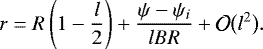
Ruderman et al. (2017) showed that P∕ψ is independent of ψ in the core region of the tube defined by the inequality r ≤ R(1 − l∕2). It follows from this result that in the core region Q = Qi(ψ∕ψi). Using this expression we obtain from Eq. (26) that ![Mathematical equation: $({\cal M}[Rw])_i = Q_i/\psi_i$](/articles/aa/full_html/2018/07/aa32396-17/aa32396-17-eq78.png) , and consequently
, and consequently
![Mathematical equation: \begin{equation*} {\cal M}[Rw] = \left(\frac{Q_i}{\psi_i} - \frac{(\rho_i - \rho)\mathrm{\Omega}^2 w_i}{RB^4}\right)[1 + {\cal O}(l)].\end{equation*}](/articles/aa/full_html/2018/07/aa32396-17/aa32396-17-eq79.png) (62)
(62)
Substituting this result in Eq. (60), integrating the obtained equation, and using the relation w = BRη yields in the leading order approximation with respect to l
 (63)
(63)
4 Calculation of the eigenmode decrement
Taking η, δη, and δP proportional to e−iωt and only keeping terms of the order of unity and l, we transform Eqs. (2) and (3) to
 (64)
(64)
and
 (65)
(65)
Recall that in these equations η is calculated in the tube core region where it is independent of ψ. Using Eqs. (4), (32), (59), and (63), we obtain
 (66)
(66)
where
![Mathematical equation: \begin{align*} &{\cal L}_1 \!=\! \frac{\mu_0\rho_e}{BR^2(\rho_i + \rho_e)}{\cal P}\!\int_{\psi_i}^{\psi_e}\!\! g(\psi)\sum_{n=1}^{\infty} \frac{[\mathrm{\Omega}_0^2 - \lambda_n(\psi_e)]\mathrm{\Phi}_n Y_n(Z)} {\mathrm{\Omega}_0^2 - \lambda_n(\psi)}\,\textrm{d}\psi \nonumber \\ &\quad\quad+\! \frac{2lB^2 Q_i}{R^2(\rho_i + \rho_e)} + \frac{\mathrm{\Omega}_0^2\eta}{\rho_i + \rho_e} \left(\frac1{BR^2}\int_{\psi_i}^{\psi_e}\!\!\rho\,d\psi - l(3\rho_i - \rho_e)\right).\end{align*}](/articles/aa/full_html/2018/07/aa32396-17/aa32396-17-eq84.png) (67)
(67)
Now we substitute Ω = Ω0 + lΩ1 in Eq. (64) and then look for a solution to Eqs. (64) and (65) in the form
 (68)
(68)
Taking into account that  , we obtain inthe leading order approximation
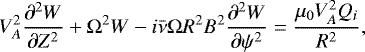
 (69)
(69)
We see that η must be an eigenfunction of the boundary value problem Eq. (69) and  the corresponding eigenvalue. Obviously, we can take η0 to be real.
In the next order approximation, we obtain
 (70)
(70)
This boundary layer problem only has solutions if its right-hand side satisfies the compatibility condition. To obtain this condition, we multiply Eq. (70) by η0, integrate the obtained equation, use the integration by parts, and use the boundary conditions. As a result, we obtain
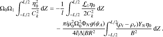 (71)
(71)
We write Ω1 = Ω1r − iΓ, where both Ω1r and Γ are real quantities. The account of Ω 1r only gives a small correction to the oscillation frequency Ω0, while Γ determines the oscillation damping rate. Below we are mainly interested in Γ, which is defined by
 (72)
(72)
We note that Γ is the scaled decrement, while the non-scaled decrement is γ = ϵΓ.
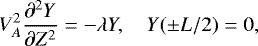
Using Eq. (35), we transform Eq. (69) to
 (73)
(73)
Comparing Eqs. (36) and (73), we conclude that  and η0 is proportional to Y n(Z) for some n. To have the proper dimension of η, we take
  . Since 1 < χ < g(ψe), it follows that
  . Then the condition that
  implies that n = N and we obtain
  and
and  . Using this result and Eqs. (4), (35), and (38), we obtain
 (74)
(74)
Using Eqs. (61) and (62) and the relation Rwi = BR2η0, we obtain in the leading order approximation
![Mathematical equation: \begin{equation*} Q_i = \frac{\rho_i\psi_i}{B^3}\big[\mathrm{\Omega}_0^2 - \lambda_N(\psi_i)\big]\eta_0.\end{equation*}](/articles/aa/full_html/2018/07/aa32396-17/aa32396-17-eq100.png) (75)
(75)
Then we obtain with the aid of Eqs. (38)–(40):
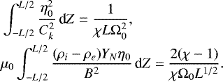
![Mathematical equation: \begin{eqnarray*} \mathrm{\Phi}_N = \int_{-L/2}^{L/2}\frac{Q_i Y_N}{R^2}\,\textrm{d}Z &=& \frac{\psi_i\big[\mathrm{\Omega}_0^2 - \lambda_N(\psi_i)\big]}{\mu_0\mathrm{\Omega}_0 L^{1/2}BR^2}\int_{-L/2}^{L/2} \frac{Y_N^2}{V_{Ai}^2}\,\textrm{d}Z \nonumber\\ &=& \frac{\psi_i\big[\mathrm{\Omega}_0^2 - \lambda_N(\psi_i)\big]}{\mu_0\mathrm{\Omega}_0 L^{1/2}BR^2}.\end{eqnarray*}](/articles/aa/full_html/2018/07/aa32396-17/aa32396-17-eq101.png) (76)
(76)
Substituting Eqs. (74) and (76) in Eq. (72) and recalling that γ = ϵlΓ and ω0 = ϵlΩ0, we reduce this equation to
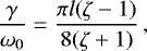
![Mathematical equation: \begin{equation*} \frac\gamma{\omega_0} = \frac{\pi\psi_i\lambda_N(\psi_i) g(\psi_A)(\chi-1)[g(\psi_A) - 1]} {2|\mathrm{\Delta}|B^2 R^4}\,.\end{equation*}](/articles/aa/full_html/2018/07/aa32396-17/aa32396-17-eq102.png) (77)
(77)
Ruderman et al. (2017) showed that in the approximation of the thin tube,  . It follows from this relation that
  . In addition, it follows from Eqs. (35), (37), and (46) that Δ = −λN(ψi)g′(ψA), where the prime indicates the derivative. It follows from Eqs. (37) and (42), and from the relation
 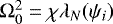 that ψA is defined by
 (78)
(78)
Then we can simplify Eq. (77) to
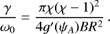 (79)
(79)
It is straightforward to verify that this expression coincides with the corresponding expression in Dymova & Ruderman (2006; see their Eq. (83)).
Now we can notice that, while to calculate ω0 and γ we need to define V Ai(z), the ratio γ∕ω0 is independent of a particular form of this function. It is also independent of the number of mode N. We recall that this result was obtained under the assumption of homogeneous stratification. It is a generalisation of a similar result previously obtained by Dymova & Ruderman (2006) for non-expanding magnetic tubes.
As an example, we consider the linear density variation in the transitional layer and take
 (80)
(80)
Using the relation  , we obtain
 (81)
(81)
It follows from Eqs. (35), (80), and (81) that
 (82)
(82)
Using this equation and Eq. (73), we obtain
 (83)
(83)
Then it follows from Eq. (78) that
 (84)
(84)
Using Eqs. (82) and (84), we obtain in the leading order approximation with respect to l
 (85)
(85)
When deriving this expression, we used the relation  . Substituting this expression in Eq. (79) and using Eq. (83) yields
 (86)
(86)
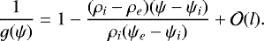
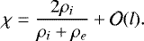
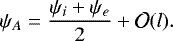
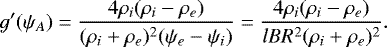
where ζ = ρi∕ρe. This expression coincides with that obtained for a non-expanding tube with the density remaining non-varying along the tube (e.g. Goossens et al. 2002). We repeat that, in accordance with the homogeneous stratification assumption ρi∕ρe = const, the ratio of the decrement to the frequency is independent of a particular law of the density variation along the tube.
5 Summary and conclusions
In this article, we studied resonant damping of kink oscillations of thin expanding and stratified magnetic flux tubes. Our analysis is based on the equations describing kink oscillations of expanding flux tubes that were derived by Ruderman et al. (2017). This system is not closed because it contains the jumps of the magnetic pressure and plasma displacement across the transitional layer where the plasma density decreases from its values in the tube core region to its value in the surrounding plasma. We derived expressions for these quantities thus closing the system.
We used the obtained jumps across the transitional layer to calculate the decrements of eigenmodes of the tube kink oscillations. We generalised the definition of homogeneous stratification formulated by Dymova & Ruderman (2006). We defined it as the condition that the ratio of densities in the tube core region and outside the tube does not vary along the tube, and the density in the transitional layer can be factorised and written as a product of two functions, one depending on the coordinate along the tube and the other depending on the magnetic flux function. Although at first sight this assumption looks artificial, in fact it is quite viable. If the temperature does not change across the tube and its vicinity, then the density variation along a magnetic line in the tube and its vicinity is the same along this line, while its absolute value can change fromline to line. The main result is that, under the assumption of homogeneous stratification, the ratio of decrement and oscillation frequency is independent of a particular form of the density and tube cross-sectional radius variation along the tube, and it is also the same for any oscillation eigenmode. This result has an important implication for coronal seismology. It enables to disregard the coronal loop expansions and density variation along the loops when using the observed damping of kink oscillations to get information about the radial structure of the loops.
Acknowledgements
M.S.R. acknowledges support from an STFC grant.
References
- Alan, W., & Wright, A. N. 1998, J. Geophys. Res., 102, 19927 [NASA ADS] [CrossRef] [Google Scholar]
- Arregui, I. 2015, Phil. Trans. R. Soc., 373, 20140261 [Google Scholar]
- Aschwanden, M. J., Fletcher, L., Schrijver, C. J., & Alexander, D. 1999, ApJ, 520, 880 [NASA ADS] [CrossRef] [Google Scholar]
- Bender, C. M., & Orszag, S. A. 1978, in Advanced Mathematical Methods for Scientists and Engineers (New York: McGraw-Hill) [Google Scholar]
- Braginskii, S. I. 1965, Rev. Plasma Phys., 1, 205 [Google Scholar]
- Chen, L., & Hasegawa, A. 1974a, Phys. Fluids, 17, 1399 [NASA ADS] [CrossRef] [Google Scholar]
- Chen, L., & Hasegawa, A. 1974b, J. Geophys. Res., 79, 1024 [NASA ADS] [CrossRef] [Google Scholar]
- Chen, L., & Hasegawa, A. 1974c, J. Geophys. Res., 79, 1033 [NASA ADS] [CrossRef] [Google Scholar]
- Coddington, E. A., & Levinson, N. 1955, Theory of Ordinary Differential Equations (New York: McGraw-Hill) [Google Scholar]
- Dymova, M. V., & Ruderman, M. S. 2006, A&A, 457, 1059 [NASA ADS] [CrossRef] [EDP Sciences] [Google Scholar]
- Edwin, P. M., & Roberts, B. 1983, Sol. Phys., 88, 179 [NASA ADS] [CrossRef] [Google Scholar]
- Erdelyi, R., & Goossens, M. 1995, A&A, 294, 575 [NASA ADS] [Google Scholar]
- Goossens, M., Hollweg, J. V., & Sakurai, T. 1992, Sol. Phys., 138, 233 [NASA ADS] [CrossRef] [Google Scholar]
- Goossens, M., Ruderman, M. S., & Hollweg, J. V. 1995, Sol. Phys., 157, 75 [NASA ADS] [CrossRef] [Google Scholar]
- Goossens, M., Andries, J., & Aschwanden, M. J. 2002, A&A, 394, L39 [NASA ADS] [CrossRef] [EDP Sciences] [Google Scholar]
- Goossens, M., Erdélyi, R., & Ruderman, M. S. 2011, Space Sci. Rev., 158, 289 [NASA ADS] [CrossRef] [Google Scholar]
- Grossmann, W., & Tataronis, J. 1973, Z. Phys., 261, 217 [NASA ADS] [CrossRef] [Google Scholar]
- Hasegawa, A., & Chen, L. 1976, Phys. Fluids, 19, 1924 [NASA ADS] [CrossRef] [Google Scholar]
- Hollweg, J. V. 1990, Comput. Phys. Rep., 12, 205 [Google Scholar]
- Hollweg, J. V., & Yang, G. 1988, Comput. Phys. Rep., 93, 5423 [Google Scholar]
- Inhester, B. 1986, J. Geophys. Res., 91, 1509 [NASA ADS] [CrossRef] [Google Scholar]
- Ionson, J. A. 1978, ApJ, 226, 650 [NASA ADS] [CrossRef] [Google Scholar]
- Ionson, J. A. 1985, Sol. Phys., 100, 289 [NASA ADS] [CrossRef] [Google Scholar]
- Kivelson, M. G., & Southwood, D. J. 1986, J. Geophys. Res., 91, 4345 [NASA ADS] [CrossRef] [Google Scholar]
- Klimchuk, J. A. 2000, Sol. Phys., 193, 53 [NASA ADS] [CrossRef] [Google Scholar]
- Korn, G., & Korn, T. 1961, Mathematical Handbook for Scientists and Engineers (New York: McGraw-Hill) [Google Scholar]
- Kuperus, M., Ionson, J. A., & Spiser, D. 1981, ARA&A, 19, 7 [NASA ADS] [CrossRef] [Google Scholar]
- Lanzerotti, L. J., Fukunishi, H., Hasegawa, A., & Chen, L. 1973, Phys. Rev. Lett., 31, 624 [NASA ADS] [CrossRef] [Google Scholar]
- Nakariakov, V. M., Ofman, L., Deluca, E. E., Roberts, B., & Davila, J. M. 1999, Science, 285, 862 [NASA ADS] [CrossRef] [PubMed] [Google Scholar]
- Ofman, L., Davila, J. M., & Steimolfson, R. S. 1994, ApJ, 421, 360 [NASA ADS] [CrossRef] [Google Scholar]
- Rickard, G., & Wright, A. J. 1995, J. Geophys. Res., 100, 3531 [NASA ADS] [CrossRef] [Google Scholar]
- Ruderman, M. S., & Erdélyi, R. 2009, Space Sci. Rev., 149, 199 [NASA ADS] [CrossRef] [Google Scholar]
- Ruderman, M. S., & Roberts, B. 2002, ApJ, 577, 475 [NASA ADS] [CrossRef] [Google Scholar]
- Ruderman, M. S., Tirry, W., & Goossens, M. 1995, J. Plasma Phys., 54, 129 [NASA ADS] [CrossRef] [Google Scholar]
- Ruderman, M. S., Verth, G., & Erdélyi, R. 2008, ApJ, 686, 694 [NASA ADS] [CrossRef] [Google Scholar]
- Ruderman, M. S., Shukhobodskiy, A. A., & Erdélyi, R. 2017, A&A, 602, A50 [NASA ADS] [CrossRef] [EDP Sciences] [Google Scholar]
- Ryutov, D. D., & Ryutova, M. P. 1976, Sov. Phys. JETP, 43, 491 [Google Scholar]
- Sakurai, H., Goossens, S., & Hollweg, Y. 1991, Sol. Phys., 133, 227 [NASA ADS] [CrossRef] [Google Scholar]
- Southwood, D. J. 1974, Planet. Space Sci., 22, 483 [NASA ADS] [CrossRef] [Google Scholar]
- Southwood, D. J., & Hughes, W. J. 1983, Space Sci. Rev., 35, 301 [NASA ADS] [CrossRef] [Google Scholar]
- Southwood, D. J., & Kivelson, M. G. 1986, J. Geophys. Res., 91, 6871 [NASA ADS] [CrossRef] [Google Scholar]
- Tataronis, J., & Grossmann, W. 1973, Z. Phys., 261, 203 [NASA ADS] [CrossRef] [Google Scholar]
- Tirry, W., & Goossens, M. 1996, ApJ, 471, 501 [NASA ADS] [CrossRef] [Google Scholar]
- Tsuneta, S., Ichimoto, K., Katsukawa, Y., et al. 2008, ApJ, 688, 1374 [Google Scholar]
- Van Doorsselaere, T., Andries, J., Poedts, S., & Goossens, M. 2004, ApJ, 606, 1223 [NASA ADS] [CrossRef] [Google Scholar]
- Verth, G., & Erdélyi, R. 2008, A&A, 486, 1015 [NASA ADS] [CrossRef] [EDP Sciences] [Google Scholar]
- Watko, J. A., & Klimchuk, J. A. 2000, Sol. Phys., 193, 77 [NASA ADS] [CrossRef] [Google Scholar]
All Figures
|
Fig. 1 Sketch of equilibrium state. |
| In the text | |
Current usage metrics show cumulative count of Article Views (full-text article views including HTML views, PDF and ePub downloads, according to the available data) and Abstracts Views on Vision4Press platform.
Data correspond to usage on the plateform after 2015. The current usage metrics is available 48-96 hours after online publication and is updated daily on week days.
Initial download of the metrics may take a while.