| Issue |
A&A
Volume 615, July 2018
|
|
|---|---|---|
| Article Number | A42 | |
| Number of page(s) | 21 | |
| Section | Interstellar and circumstellar matter | |
| DOI | https://doi.org/10.1051/0004-6361/201731395 | |
| Published online | 10 July 2018 | |
Spectropolarimetry of Galactic stars with anomalous extinction sightlines★
1
European Southern Observatory,
Karl-Schwarzschild-Str. 2,
85748
Garching b. München,
Germany
e-mail: This email address is being protected from spambots. You need JavaScript enabled to view it.
2
Korea Astronomy and Space Science Institute,
Daejeon
34055,
Korea
e-mail: This email address is being protected from spambots. You need JavaScript enabled to view it.
3
Korea University of Science and Technology,
217 Gajungro,
Yuseong-gu,
Daejeon
34113,
Korea
4
Max-Planck-Institut für Astrophysik,
Karl-Schwarzschild-Str. 1,
85741
Garching b. München,
Germany
5
INAF-Osservatorio Astronomico di Padova,
Vicolo dell’Osservatorio 5,
35122
Padova,
Italy
6
Anton Pannekoek Institute for Astronomy, University of Amsterdam,
1090
GE Amsterdam,
The Netherlands
7
MAS—Millennium Institute of Astrophysics,
Casilla 36-D,
7591245
Santiago,
Chile
8
Instituto de Astrofísica, Pontificia Universidad Católica de Chile,
Casilla 306,
Santiago 22,
Chile
9
University of Zagreb, Faculty of Electrical Engineering and Computing, Department of Applied Physics,
Unska 3,
10000
Zagreb,
Croatia
10
Ruđer Bošković Institute,
Bijenička cesta 54,
10000
Zagreb,
Croatia
11
Max-Planck-Institut für Astronomie,
Königstuhl 17,
69117
Heidelberg,
Germany
Received:
18
June
2017
Accepted:
20
March
2018
Abstract
Highly reddened type Ia supernovae (SNe Ia) with low total-to-selective visual extinction ratio values, RV, also show peculiar linear polarization wavelength dependencies with peak polarizations at short wavelengths (λmax ≲ 0.4 μm). It is not clear why sightlines to SNe Ia display such different continuum polarization profiles from interstellar sightlines in the Milky Way with similar RV values. We investigate polarization profiles of a sample of Galactic stars with low RV values, along anomalous extinction sightlines, with the aim to find similarities to the polarization profiles that we observe in SN Ia sightlines. We undertook spectropolarimetry of 14 stars, used archival data for 3 additional stars, and ran dust extinction and polarization simulations (by adopting the picket-fence alignment model) to infer a simple dust model (size distribution, alignment) that can reproduce the observed extinction and polarization curves. Our sample of Galactic stars with low RV values and anomalous extinction sightlines displays normal polarization profiles with an average λmax ~ 0.53 μm, and is consistent within 3σ to a larger coherent sample of Galactic stars from the literature. Despite the low RV values of dust toward the stars in our sample, the polarization curves do not show any similarity to the continuum polarization curves observed toward SNe Ia with low RV values. There is a correlation between the best-fit Serkowski parameters K and λmax, but we did not find any significant correlation between RV and λmax. Our simulations show that the K–λmax relationship is an intrinsic property of polarization. Furthermore, we have shown that in order to reproduce polarization curves with normal λmax and low RV values, a population of large (a ≥ 0.1μm) interstellar silicate grains must be contained in the dust composition.
Key words: polarization / ISM: general / dust, extinction / supernovae: general / galaxies: ISM
The reduced spectra are only available at the CDS via anonymous ftp to cdsarc.u-strasbg.fr (130.79.128.5) or via http://cdsarc.u-strasbg.fr/viz-bin/qcat?J/A+A/615/A42
© ESO 2018
1 Introduction
The motivation to study anomalous sightlines toward highly reddened Galactic stars derives from type Ia supernova (SN) observations that show peculiar extinction curves with very low RV values, as well as peculiar polarization wavelength dependencies (polarization curves).
Past studies that included large samples of SNe Ia showed that the total-to-selective visual extinction ratio, RV, of dust in type Ia SN host galaxies ranges from 1 to 3.5 and is in most cases lower than the average value of Milky Way dust, RV ~ 3.1 (Riess et al. 1996; Phillips et al. 1999; Altavilla et al. 2004; Reindl et al. 2005; Conley et al. 2007; Wang et al. 2006; Goobar 2008; Nobili & Goobar 2008; Kessler et al. 2009; Hicken et al. 2009; Folatelli et al. 2010; Lampeitl et al. 2010; Mandel et al. 2011; Cikota et al. 2016).
Observations of individual highly reddened SNe Ia also reveal host galaxy dust with low RV values, for instance, RV = 2.57 for the lineof sight of SN 1986G (Phillips et al. 2013), RV ~ 1.48 for SN 2006X (Wang et al. 2008), RV = 1.20
  for SN 2008fp (Phillips et al. 2013), and
  = 1.64 ± 0.16 for SN 2014J (Foley et al. 2014).
Linear (spectro)polarimetric observations of these four SNe also display anomalous interstellar polarization curves (Patat et al. 2015), steeply rising toward blue wavelengths. Patat et al. (2015) fitted their observations with a Serkowski curve (Serkowski et al. 1975) to characterize the polarization curves.
The Serkowski curve is an empirical wavelength dependence of interstellar linear polarization:
![Mathematical equation: \begin{equation*}\frac{P(\lambda)}{P_{\mathrm{\textrm{max}}}} \,=\, \exp \left[-K \mathrm{ln}^2 \left( \frac{\lambda_{\mathrm{\textrm{max}}}}{\lambda} \right) \right] \end{equation*}](/articles/aa/full_html/2018/07/aa31395-17/aa31395-17-eq4.png) (1)
(1)
The wavelength of peak polarization, λmax, depends on the dust grain size distribution. For an enhanced abundance of small dust grains, λmax moves to shorter wavelengths, and for an enhanced abundance of large dust grains, it moves to longer wavelengths. Thus, linear spectropolarimetry probes the alignment of dust grains and the size distribution of the aligned dust grains.
Patat et al. (2015) found that the polarization curve of all 4 SNe display an anomalous behavior, with λmax ~ 0.43 μm for SN 1986G, and λmax ≲ 0.4 μm for SN 2006X, SN 2008fp, and SN 2014J. Because SNe Ia have a negligible intrinsic continuum polarization (Wang & Wheeler 2008), the anomalous polarization curves likely have to be associated with the properties of host galaxies dust. Zelaya et al. (2017) expanded the sample of 4 SNe Ia investigated in Patat et al. (2015), and presented a study of 19 type Ia SNe. They grouped the SNe into the “sodium-sample”, consisting of 12 SNe that show higher continuum polarization values and interstellar Na I D lines at the redshift of their host galaxies, and the “non-sodium-sample” with no rest-frame Na I D lines and smaller peak polarization. Eight sodium-sample SNe have λmax ≲ 0.4 μm, and their polarization angles are aligned with the spiral arms of their host galaxies, which is evidence that the polarizing dust is likely located in their host galaxies and aligned due to the magnetic fields of the host galaxies. The non-sodium-sample SNe are less strongly polarized, with Pmax ≲ 0.5%, have λmax values similar to the common Galactic dust (with λmax ~ 0.55 μm), and their polarization angles do not align with host-galaxy features, which might be interpreted as the continuum polarization being produced by the Galactic foreground dust.
It is not understood why these reddened SN Ia sightlines show such a different polarization profile compared to the typical Milky Way dust. A natural explanation is that the composition of dust in the SN Ia host galaxies is different from that in the Galaxy.
However, there are alternative explanations. Scattering might explain the low RV values as well as the peculiar polarization profiles. As illustrated by Patat et al. (2015) (see their Fig. 6), the polarization profile of SN 2006X may, in addition to the Serkowski component, also have a component induced by Rayleigh scattering. However, if a light echo propagates through local dust, we expect to observe variability in RV and polarization (Wang 2005), which is usually not the case (see Fig. 4 in Zelaya et al. 2017). Yang et al. (2017) used observations made with the Hubble Space Telescope (HST) to map the interstellar medium (ISM) around SN 2014J through light echoes. These authors observed two echo components: a diffuse ring and a luminous arc, produced through dust scattering of different grain sizes. From the wavelength dependence of the scattering optical depth, the arc dust favors a low RV value of ~1.4, which is consistent with the RV measured along the direct line of sight, while the ring is consistent with a common Milky Way RV ~ 3 value.
Another interesting explanation for the peculiar SNe Ia sightlines is given by Hoang (2017), who simultaneously fit a two-component (interstellar and circumstellar) extinction and polarization model to photometric and (spectro-) polarimetricobservations of SNe 1986G, 2006X, 2008fp, and 2014J to investigate the grain size distribution and alignment functions of dust along these lines of sights. Hoang (2017) were able to reproduce the observational data of SN 1986G and SN 2006X by assuming an enhanced abundance of small silicate grains in the interstellar dust only, while in the case of SN 2014J, a contribution of circumstellar (CS) dust must be accounted for. In the case of SN 2008fp, Hoang (2017) found that the alignment of small dust grains must be as efficient as that of large grains, but the existence of CS dust is uncertain. Hoang (2017) suggested that the enhanced abundance of small silicate grains might be produced by cloud collisions driven by the SN radiation pressure. Strong SN radiation might also induce efficient alignment of small grains via the radiative torque mechanism. However, in the case of alignment via the radiative torque mechanism, the polarization angle alignment with host-galaxy features remains unexplained.
The aim of this work is to investigate Galactic stars with low RV values with spectropolarimetry, in order to possibly find similarities to the polarization curves observed toward SNe Ia. Numerical simulations are used to infer general properties of interstellar dust toward these stars by simultaneously fitting to extinction curves with low RV values and normal polarization curves.
The paper is structured as follows: in Sect. 2 we describe our sample of stars, in Sect. 3 the instruments and observing strategies, in Sect. 4 we present the data processing and results, in Sect. 5 the analysis of the observations, in Sect. 6 we run simulations in order to interpret the observed data, in Sect. 7 we discuss the results, and finally we summarize and conclude in Sect. 8.
2 Target sample
We selected our targets from the samples presented by Mazzei & Barbaro (2008, 2011). Mazzei & Barbaro (2011) obtained 785 extinction curves for sightlines with E(B − V) ≥ 0.2 mag (Savage et al. 1985), observed with the Astronomical Netherlands Satellite (ANS) in five UV bands (1/λ = 6.46, 5.56, 4.55, 4.01 and 3.04 μm−1; Wesselius et al. 1982). They combined the UV observations with Two-Micron All-Sky Survey (2MASS) observations in the near-infrared J, H, and K bands, applied a least-squares fit of the standard Cardelli et al. (1989) extinction curve (CCM) with different RV values, and determined the residual differences between the observed values and best-fit CCM curve at five UV wavelengths. The curves were classified as anomalous if at least one UV wavelength deviated by more than 2σ from the best-fit standard CCM curve. Twenty curves with weaker UV bumps and steeper far-UV slopes (type A), or with stronger bumps and smoother far-UV rises (type B) compared to their best-fit CCM curve, were analyzed in Mazzei & Barbaro (2008). Mazzei & Barbaro (2011) focus on 64 lines of sight for which the corresponding best-fit CCM curve is always well below (≥ 2σ) or well above the observed data (type C curves), with some exception at 1/λ = 3.01 for five curves (see bottom panel of Fig. 1 in Mazzei & Barbaro 2011). They conclude that the sightlines characterized by anomalous type C extinction curves require lower dust abundances than environments characterized by normal CCM extinction curves.
From these 64 anomalous lines of sight, we selected 14 lines of sight with the lowest RV values and observed them with the FOcal Reducer and low dispersion Spectrograph (FORS2), the Asiago Faint Object Spectrograph and Camera (AFOSC), and the Calar Alto Faint Object Spectrograph (CAFOS). The observed targets are listed in Table 1. Additionally, we used archival HPOL data for 3 stars.
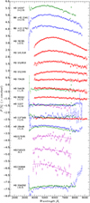 |
Fig. 1 Weighted averages of observed polarization curves for all science targets, derived with different instruments. The red circles show observations performed with FORS2, blue triangles with CAFOS, green squares with AFOSC, and left-pointingpurple triangles with HPOL. The full lines denote the Serkowski fits, as parametrized in Table 3. |
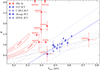 |
Fig. 2 Stars with anomalous extinction sightlines in the λmax-K plane. Blue shows stars with anomalous sightlines observed with FORS2 (circles), CAHA (right pointing triangles), AFOSC (squared), and HPOL (left-pointing triangles). The solid blue line represents the linear best fit to the sample, and its 1σ deviation (dotted). The dashed black line traces the Whittet et al. (1992) relation and its 3σ uncertainty(dotted). For comparison, a sample of SNe Ia from Patat et al. (2015) and Zelaya et al. (2017; see Appendix B) are marked with stars and red contours, which indicate the 10 and 20 σ confidence levels for SN 2008fp and SN 2014J. |
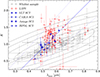 |
Fig. 3 Comparison of our sample of stars with anomalous extinction sightlines (blue symbols) to the Whittet et al. (1992) sample (gray squares) and the LIPS sample (Bagnulo et al. 2017, red circles). The gray ellipses represent 1–5σ confidence levels for the Whittet et al. (1992) sample. The dashed black line traces the Whittet et al. (1992) relation and its 1σ uncertainty (dotted). |
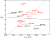 |
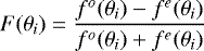
Fig. 4 RSi–λmax relationship. The red dots represent stars observed with FORS2, AFOSC, and CAFOS, and the black dots show seven additional measurements from HPOL or from the literature. The red dashed line is the linear least-squares fit to the red dots, and the black solid line is the linear least-squares fit to all data. |
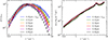 |
Fig. 5 Left panel: best-fit models vs. generated (i.e., constructed) polarization curves for six different models described by λmax. Right panel: best-fit models vs. generated extinction curves with a low RV = 2.5. Filled circles show the generated data, and solid lines show our best-fit models. |
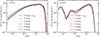 |
Fig. 6 Best-fit grain size distribution for silicate (left panel) and carbonaceous grains (right panel). Six different models described by λmax are considered. Large silicate grains of size a ≥ 0.1μm are present to reproduce normal λmax. |
Observed stars.
3 Instruments and methods
We observed our targets using three different instruments and telescopes: the FOcal Reducer and low dispersion Spectrograph (FORS2) in spectropolarimetric mode (PMOS) mounted on the UT1 Cassegrain focus of the Very Large Telescope (VLT) in Chile; the Asiago Faint Object Spectrograph and Camera (AFOSC) mounted at the 1.82 m Copernico telescope at the Asiago Observatoryin northern Italy; and the Calar Alto Faint Object Spectrograph (CAFOS) mounted at the Calar Alto 2.2 m telescope in Andalusia, Spain.
The characteristics of the instruments and corresponding differences in the data reduction are described in the following subsections.
3.1 FORS2 at the VLT
FORS2 in PMOS mode is a dual-beam polarimeter. The spectrum produced by the grism is split by the Wollaston prism into two beams with orthogonal directions of polarization: ordinary (o) and extraordinary (e) beam. The data used in this work were obtained with the 300V grism, with and without the GG435 filter, and with the half-wave retarder plate positioned at angles of 0°, 22.5°, 45°, and 67.5° (Program ID: 094.C-0686). The half-wave retarder plate angle is measured between the acceptance axis of the ordinary beam of theWollaston prism (which is aligned to the north-south direction) and the fast axis of the retarder plate.
The data were reduced using standard procedures in IRAF. Wavelength calibration was achieved using He-Ne-Ar arc lamp exposures. The typical RMS accuracy is ~0.3 Å. The data were bias subtracted, but not flat-field corrected. However, the effects of improper correction were minimized by taking advantage of the redundant number of half-wave positions (see Patat & Romaniello 2006).
Ordinary and extra-ordinary beams were extracted in an unsupervised way using the PyRAF apextract.apall procedure, with a fixed aperture size of 10 pixels. The synthetic broadband polarization degree was computed by integrating the total flux weighted with Bessel’s BVRI passband filters. We binned the spectra in 50 Å bins, in order to obtain a higher signal-to-noise ratio (S/N), and calculated the Stokes parameters Q and U, polarization degree P, and polarization angle θP as a function of wavelength.
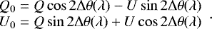
The Stokes parameters Q and U were derived via Fourier transformation, as described in the FORS2 User Manual (ESO 2015):
 (2)
(2)
where F(θi) are the normalized flux differences between the ordinary (fo) and extra-ordinary (fe) beams:
 (3)
(3)
at different half-wave retarder plate position angles θi = i * 22.5°.
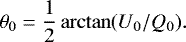
Although FORS2 is equipped with a super-achromatic half-wave plate, residual retardance chromatism is present. The wavelength dependent retardance offset (Δθ(λ)) is tabulated in the FORS2 User Manual. The chromatism was corrected through the following rotation of the Stokes parameters:
 (4)
(4)
Finally we calculated the polarization:
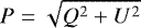 (5)
(5)
and the polarization angle:
 (6)
(6)
The reliability of data obtained with FORS2 is demonstrated in Cikota et al. (2017a). They used archival data of polarized and unpolarized stars to test the stability and capabilities of the spectropolarimetric mode (PMOS) of the FORS2 instrument, and found a good temporal stability since FORS2 was commissioned, and a good observational repeatability of total linear polarization measurements with an RMS ≲0.21%. Cikota et al. (2017a) also found a small (≲0.1%) instrumental polarization and fit linear functions to correct Stokes Q and U, which we applied to the FORS2 data in this work.
3.2 AFOSC at the 1.82 m Copernico telescope
Spectropolarimetry with AFOSC was obtained using a simple combination of two Wollaston prisms and two wedges, a grism, and a slit mask of 2.5 arcsec wide and 20 arcsec long slitlets. This configuration permits measurements of the polarized flux at four polarimetric channels simultaneously, that is, at angles 0, 45, 90 and 135 degrees, without the need of a half-wave retarder plate (Oliva 1997). For any given rotator adapter angle θi, four fluxes can be measured. We group them into two groups, which we call ordinary (O) and extraordinary (E). We indicate them as fO1,i, fE1,i and fO2,i, fE2,i. We used them to indicate the generic four beams f0, f90 and f45, f135, respectively.
However, in order to remove possible instrumental problems (i.e., imperfect beam splitting, flat fielding, etc.) it is convenient to obtain at least two sets of data. This can be achieved by rotating the instrument by 90 degrees with respect to the sky, so that a pair-wise swap between the corresponding polarimeter channels, 0 to 90 and 45 to 135 degrees, is performed.
The final Q and U were obtained via the Fourier approach:
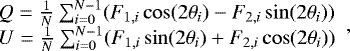 (7)
(7)
where N is the number of rotator adapter angles,  , and F1,i and F2,i are normalized flux ratios:
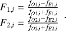 (8)
(8)
Finally, we calculated the polarization degree and angle as given in Eqs. (5) and (6) respectively.
3.3 CAFOS at the Calar Alto 2.2 m telescope
CAFOS is a dual-beam polarimeter, similar to FORS2 in PMOS mode, composed of a half-wave retarder followed by a Wollaston prism that splits the incoming beam into an ordinary and an extra-ordinary beam. The data processing is as described for FORS2 in Sect. 3.1.
The CAFOS instrument was characterized in Patat & Taubenberger (2011). They used polarized standard starsto quantify the HWP chromatism, which causes a peak-to-peak oscillation of ~11 degrees. From observations of unpolarized standard stars, they found an instrumental polarization likely produced by the telescope optics, which appears to be additive. The instrumental polarization is ~0.3% between 4000 Å and 8600 Å, and grows to ~0.7% below 4000 Å. It can be removed by subtracting the instrumental components in the Q–U Stokes plane. After correcting for the HWP chromatism and instrumental polarization, Patat & Taubenberger (2011) concluded that an accuracy of ~0.1% can be reached with four HWP angles and a sufficient S/N.
4 Data processing and results
The data were obtained with FORS2 in eight different nights between 2014-10-10 and 2015-02-06 (Program ID: 094.C-0686), with CAFOS in the night of 2015-04-29, and with AFOSC in five nights at three observing runs starting on 2015-02-09, 2015-03-09, and 2016-08-02.
4.1 Standard stars
We investigate the accuracy and reliability of the instruments using unpolarized and polarized standard stars. Cikota et al. (2017a) used archival data of eight unpolarized standard stars observed at 40 epochs between 2009 and 2016 to test the stability and capabilities of the spectropolarimetric mode (PMOS) of the FORS2 instrument. They showed that the polarization degree and angle are stable at the level of ≲0.1% and ≲0.2 degrees, respectively. They found a small (≲0.1%) wavelength-dependent instrumental polarization and derived linear functions for the Stokes Q and U, which we applied to the observed Stokes parameters. In this paper, we therefore focus on unpolarized and polarized standard stars observed with CAFOS and AFOSC.
Two unpolarized standard stars (HD 144579, and HD 90508), and two polarized standard stars (HD 154445 and HD 43384) were observed with CAFOS. We did not find any significant instrumental polarization in the CAFOS observations, and the polarization values are consistent with the literature. The results are given in Sect. A.1.
We used observations of three unpolarized standard stars to investigate possible instrumental polarization of AFOSC: HD 90508, HD 39587 and HD 144579; and three polarized standard stars to test the reliability: HD 43384, HD 21291, and HD 198478. We did not detect any significant instrumental polarization, but the polarization degrees of polarized stars observed at different epochs vary by ~0.3%. The inconsistencies might be caused by diffraction of light from the edge of the slit (see Keller C.U. in Trujillo-Bueno et al. 2002, p. 303) or by an inaccuracy of the instruments rotation angle (see Bagnulo et al. 2017). The results are given in Sect. A.2.
4.2 FORS2 science data
FORS2 is the most stable instrument used in this work, and we are confident that the data gained with FORS2 are accurate and can be used as reference for comparison to other instruments (see Cikota et al. 2017a). Eight stars with anomalous extinction sightlines were observed with FORS2 (see Table 1). HD 54439 was also observed with AFOSC, and HD 137569 was observed with all three instruments, FORS2, CAFOS, and AFOSC, which we briefly discuss in this section. HD 78785, HD 141318, HD 152853, HD 152245, HD 73420, and HD 96042 were observed only with FORS2.
We extracted the spectra and calculated the polarization dependencies as described in Sect. 3.1. The correction for the instrumental polarization determined in Cikota et al. (2017a) was also applied to Stokes Q and U. The targets have been observed with and without the GG435 filter. The GG435 filter blocks the blue light and thus prevents the second order spectrum. However, the effect in polarization is very small, and significant only for very blue spectral energy distributions and when measuring line polarization (Patat et al. 2010). For our reddened targets, the second-order polarization is negligible. Therefore, for wavelengths λ > 4250Å, we calculated the weighted mean of all epochs, and for wavelengths λ < 4250Å, we calculated the weighted mean of all epochs taken without the GG435 filter. We then merged both ranges to one polarization spectrum and parameterized it by fitting a Serkowski curve (Eq. (1)) to the data. The individual results can be found in Table C.1. The polarization dependencies are shown in Fig. 1, and the Serkowski parameters are given in Table 3.
HD 137569 is an interesting case because it has relatively high reddening E(B − V) ~ 0.40 mag (Mazzei & Barbaro 2011), but its polarization degree is consistent with zero (Fig. 1). Its mean Stokes Q and U are − 0.07 ± 0.05% and 0.01 ± 0.03%. HD 137569 was also observed with CAFOS and AFOSC, and the results are consistent with the FORS2 observations. Furthermore, HD 137569 is a spectroscopic binary with a period of 529.8 days, and shows observational signatures normally seen in post-AGB stars (Giridhar & Arellano Ferro 2005). This is interesting, because sightlines to post-AGB stars usually show continuum polarization (Johnson & Jones 1991).
λmax and Pmax from the literature.
Final Serkowski parameters.
4.3 CAFOS science data
Six stars with anomalous extinction sightlines were observed with CAFOS. HD 1337 and HD 28446 were also observed with AFOSC, and HD 137569 was additionally observed with both FORS2 and AFOSC (see also Sect. 4.2). BD +45 3341, BD +23 3762, and HD 194092 were observed only with CAFOS.
After the beam extraction using the apextract.apall procedure of PyRAF, we binned the spectra into 100 Å wide bins and calculated the polarization as described in Sect. 3.3. Finally, we fit the Serkowski curve in the range between 3800–8600 Å. The individual results are listed in Table C.2. The polarization dependencies are shown in Fig. 1, and the Serkowski parameters are listed in Table 3. Below we discuss the interesting cases.
4.3.1 HD 1337
HD 1337 is a close spectroscopic binary star, with a period of 3.52 days (Pourbaix et al. 2004), and may be surrounded by a common-envelope, where significant dust amounts may be produced (Lü et al. 2013). HD 1337 has a constant polarization degree of ~0.55%. The CAFOS observations are also consistent with the AFOSC observations, which confirms the polarization wavelength independence (see Fig. 1). In this case, the Serkowski fit is not meaningful.
4.3.2 HD 194092
For HD 194092, the polarization observed by CAFOS follows a Serkowski curve until 7250 Å, when it starts to steeply increase from p ~ 0.5% to p ~ 2% at 8650 Å. The steep increase is not present in the AFOSC observations and is an artifact that we cannot explain. Thus, we fit the Serkowski curve in the range from 3800–7250 Å, and find λmax = 5728 ± 235Å, pmax = 0.64 ± 0.01% and K = 1.46 ± 0.47.
4.4 AFOSC science data
Six stars with anomalous extinction sightlines have been observed with AFOSC. HD 28446, HD 1337, and HD 194092 were also observed with CAFOS and HD 54439 with FORS2, while HD 137569 was additionally observed with CAFOS and FORS2 (see also Sect. 4.2). HD 14357 was observed only with AFOSC.
We extracted the beams from 3400–8150 Å using the same standard procedures in IRAF as for the extraction of FORS2 and CAFOS spectra, binned the data to 100 Å wide bins, and calculated the polarization as described in Sect. 3.2. The polarization spectra from 3500–8150 Å were fitted with a Serkowski curve, excluding the range from 7500–7700 Å, which is contaminated by the telluric O2 line.
The unpolarized standard stars are consistent with zero, which implies that there is no significant instrumental polarization (Sect. A.2). However, based on the measurements of the polarized standard stars HD 43384 and HD 21291 (see Sect. A.2), which show a negative offset compared to the literature values, we conclude that the accuracy of the polarization measurements is within ~0.4%. HD 28446 and HD 54439 show an offset of ~−0.1% compared to the results achieved with CAFOS and FORS2, respectively, while the measurements of HD 1337 are consistent with the CAFOS measurements, and the measurements of HD 137569 are consistent with the FORS2 and CAFOSmeasurements (Fig. 1). The individual results are listed in Table C.3.
HD 14357 is the only AFOSC target that has no common observations with another instrument. From the Serkowski fit, we determined λmax = 4942 ± 31Å, pmax = 3.69 ± 0.01% and K = 0.91 ± 0.04. Based on HD 43384 and other polarized stars, the λmax and K values are probably accurate, while there might be a negative offset, ≲0.4%, to the true value of pmax.
4.5 HPOL science data
We found archival data for HD 1337 (which was also observed with CAFOS and AFOSC), and three additional stars of the Mazzei &Barbaro (2011) sample in the University of Wisconsin’s Pine Bluff Observatory (PBO) HPOL spectropolarimeter (mounted at the 0.9 m f/13.5 cassegrain) data set. All targets were observed prior to the instrument update in 1995, when HPOL was providing spectropolarimetry over the range of 3200 Å to 7750 Å, with a spectral resolution of 25 Å. A half-wave plate was rotated to eight distinct angles to provide the spectropolarimetric modulation (Wolff et al. 1996).
The HPOL data are available in the Mikulski Archive for Space Telescopes (MAST) at the Space Telescope Science Institute. They include the Stokes parameters Q and U, and the error as a function of wavelength.
We calculated the polarization and polarization angle using Eqs. (5) and (6), and fit a Serkowski curve to the data (Eq. (1)). The results are given in Table 3.
4.6 Literature science data
We found polarization measurements in the literature (Coyne et al. 1974; Serkowski et al. 1975) of eight stars of the Mazzei & Barbaro (2011) sample. Three of the stars have been observed in this work with FORS2, AFOSC, or CAFOS, and for two stars, we found archival HPOL data. The stars were observed with broadband polarimeters and were characterized by fitting the Serkowski curve (Table 2). However, because the authors assumed a fixed K = 1.15, we could only partially use the measurements from Coyne et al. (1974) and Serkowski et al. (1975) in our further analysis.
5 Data analysis
Figure 2 shows the sample of 15 anomalous sightlines (listed in Table 3, excluding HD 137569 and HD 1337), compared to a sample of Galactic stars observed by Whittet et al. (1992) and a sample SNe Ia from Patat et al. (2015) and Zelaya et al. (2017; see Appendix B).
Mazzei & Barbaro (2011) used models of Weingartner & Draine (2001, hereafter WD01) and the updates by Draine & Li (2007) to compute grain-size distributions for spherical grains of amorphous silicate and carbonaceous grains consisting of graphite grains and polycyclic aromatic hydrogenated (PAH) molecules. As described in Mazzei & Barbaro (2011), they best-fit the extinction curves with models as described above (Sect. 2) to derive the properties of the dust in terms of dust-to-gas ratios, abundance ratios, and small-to-large grain size ratios of carbon and of silicon. They excluded HD 1337 (a W UMa type variable) and HD 137569 (a post-AGB star) from their analysis before performing the modeling because of the extremely low CCM RV values of these sightlines, RV ≈ 0.6 and RV ≈ 1.1, respectively, which are well outside the range explored by CCM extinction curves.
We combined the λmax values from this work with the results of WD01 best-fit models of Mazzei & Barbaro (2011, their Table 4), and computed the Pearson correlation coefficient, ρ, and the p-value for testing the non-correlation between λmax and their derived dust-to-gas ratio ( ), carbon and silicon abundances compared to solar values (
 ,
,  ), RV value, the ratio between reddening and total hydrogen column density (
 ), and small-to-large grain size ratios of carbon (RC) and silicon (RSi). They considered grains as small if their size is ≤0.01 μm, and otherwise as large. We note that a detailed analysis and discussion of the WD01 best-fit model results for the whole sample of 64 anomalous sightlines is given in Mazzei & Barbaro (2011).
The strongest correlation we found between λmax and RSi, with a correlation factor of ρ = 0.50, and the p-value for testing non-correlation of p = 0.10, while there is no correlation between λmax and other parameters (ρ ≲ 0.25). We also added three stars observed by HPOL and three stars from the literature (Coyne et al. 1974; Serkowski et al. 1975) to the sample and repeated the same correlation tests. These additional stars have anomalous extinction sightlines (Mazzei & Barbaro 2011), but higher RV values than our observed sample (see Table 4). After including the three HPOL observations and three stars from literature, the RSi − λmax correlation factor drops to ρ = −0.06. The RSi − λmax correlation is shown in Fig. 4. However, these results should be taken with care because when we fit the data, we assumed no uncertainty in RSi. This may be problematic because the realistic uncertainty in the model quantities should be considerable, probably larger than in λmax, which is a simple measurement. In this way, the fit is strongly driven by the few stars with very low λmax errors. The relationship is further discussed in Sect. 7.7.
Observational data and results of modeling
6 Dust properties inferred from simulations
The properties of dust grains toward the considered stars were obtained in Mazzei & Barbaro (2008), where the authors performed theoretical model fitting to the anomalous extinction curves. The authors found that to reproduce the anomalous extinction, silicate grains must be concentrated in small sizes of a < 0.1 μm (see also Mazzei & Barbaro 2011). Such small silicate grains cannot reproduce the normal λmax that is measured. In this section, we therefore infer the essential dust properties (i.e., size distribution and alignment) by fitting both extinction curves with low RV values and normal polarization curves. The results are used to interpret the λmax–K relationship, the deviation of K from the average value from a sample of “normal” Galactic stars, and to test the relationship between RSi and λmax.
6.1 Dust model and observational constrains
6.1.1 Dust model: size distribution
We adopted a mixed-dust model consisting of astronomical silicate and carbonaceous grains (see Weingartner & Draine 2001, hereafter WD01). The same size distribution model was also used in Mazzei & Barbaro (2011). We assumed that grains have oblate spheroidal shapes, and let a be the effective grain size defined as the radius of the equivalent sphere with the same volume as the grain.
Following WD01, the grain size distribution of dust component j is described by an analytical function:
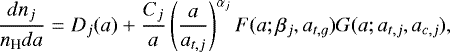 (9)
(9)
where a is the grain size, j = sil, carb for silicate and carbonaceous compositions, Dj(a) is the size distribution for very small grains, at,j, ac,j are model parameters, and Cj is a constant determined by the total gas-to-dust mass ratio.
The coefficients F and G read

and
![Mathematical equation: \begin{eqnarray}G(a;a_{t,j},a_{c,j})&=&1 {~\rm for~} a<a_{t,j},\\ G(a;a_{t,j},a_{c,j})&=&\exp\left(-[(a-a_{t,j})/a_{c,j}]^{3}\right) {~\rm for~} a>a_{t,j}. \end{eqnarray}](/articles/aa/full_html/2018/07/aa31395-17/aa31395-17-eq19.png)
The term Dj = 0 for j = sil. For very small carbonaceous grains (i.e., PAHs), Dj(a) is described by a log-normal size distribution containing a parameter bC that denotes the fraction of C abundance present in very small sizes (see WD01 for more detail). Thus, the grain size distribution is completely described by a set of 11 parameters: αj, βj, at,j, ac,j, and Cj, where j = sil, carb for silicate and carbonaceous compositions, and bC.
6.1.2 Dust model: alignment function
Let fali be the fraction of grains that are perfectly aligned with the symmetry axis â1 along the magnetic field B. The fraction of grains that are randomly oriented is thus 1 − fali. To parameterize the dependence of fali on the grainsize, we introduce the following function:
![Mathematical equation: \begin{eqnarray*} f_{\textrm{ali}}(a;a_{\textrm{ali}},f_{\textrm{min}}, f_{\textrm{max}}) = f_{\textrm{min}} + \left[1-\exp\left(-\frac{a}{a_{\textrm{ali}}}\right)^{3} \right] \left(f_{\textrm{max}}-f_{\textrm{min}}\right),\nonumber\\\end{eqnarray*}](/articles/aa/full_html/2018/07/aa31395-17/aa31395-17-eq20.png) (14)
(14)
where aali describes the minimum size of aligned grains, fmax describes the maximum degree of grain alignment, and fmin accounts for some residual small degree of alignment of very small grains. This alignment function reflects the modern understanding of grain alignment, where large grains are efficiently aligned by radiative torques (see, e.g., Hoang & Lazarian 2016) and small grains are weakly aligned by paramagnetic relaxation (Hoang et al. 2014).
6.2 Extinction and polarization model
6.2.1 Extinction
The extinction of starlight due to scattering and absorption by interstellar grains in units of magnitude is given by
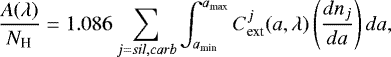 (15)
(15)
where Cext is the extinction cross-section, amin and amax are the lower and upper cutoffs of the grain size distribution, and NH is the total gas column density along the sightline.
6.2.2 Polarization
Modeling the starlight polarization by aligned grains is rather complicated because it requires a detailed knowledge of the orientation of grains with the magnetic field and the magnetic field geometry along the line of sight. Specifically, a realistic modeling needs to take into account the nutation of the grain symmetry axis â1 around the angular momentum J, the precession of J around B, and the distribution function of the cone angle between J and B (Hong & Greenberg 1980; see Voshchinnikov 2012 for a review). However, an analytical distribution function for the cone angle is not known for the popular alignment mechanism by radiative torques (see Lazarian et al. 2015 and Andersson et al. 2015 for latest reviews). Therefore we adopted a picket-fence (PF) alignment model to compute the polarization, as used in previous works (Kim & Martin 1995; Draine & Allaf-Akbari 2006; Draine & Fraisse 2009; Hoang et al. 2013, 2014). The essence of the PF model is as follows.
First, the oblate grain is assumed to be spinning around the symmetry axis â1 (i.e., having perfect internal alignment). The magnetic field B is assumed to lie in the plane of the sky  with
with  , and the line of sight is directed along
  . Therefore, the polarization cross-section contributed by the perfectly aligned grains is Cx − Cy = (C∥− C⊥)fali, where C∥ and C⊥ are the cross-section for the incident electric field parallel and perpendicular to the symmetry axis, respectively (see Hoang et al. 2013). Of (1 − fali) randomly oriented grains, the fraction of grains that are aligned with
  are equal, of (1 − fali)∕3. The total polarization produced by grains with
  is then Cx − Cy = (C∥− C⊥)(fali + (1 − fali)∕3). The polarization by grains aligned with
  is (1 − fali)∕3(C∥− C⊥)∕3. Thus, the total polarization cross-section is Cx − Cy = (C∥− C⊥)[(1 + 2fali) − (1 − fali)]∕3 = Cpolfali.
Because graphite grains are not aligned with the magnetic field (Chiar et al. 2006; Hoang & Lazarian 2016), we assumed that only silicate grains are aligned, while carbonaceous grains are randomly oriented. Therefore, the degree of polarization of starlight due to differential extinction by aligned grains along the line of sight is computed by
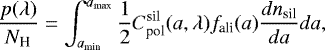 (16)
(16)
where  is the polarization cross-section of silicate oblate grains, and fali is given by Eq. (14). Here we take Cext and Cpol computed for different grain sizes and wavelengths from Hoang et al. (2013).
We note that magnetic fields may be varying for the different stars. However, we here do not attempt to infer a dust model for each specific sightline. Instead, we only attempt to infer the general features of dust size distribution and alignment functions for this group of stars with anomalous RV and normal λmax. Detailed modeling for each specific star is beyond the scope of this paper.
6.3 Numerical modeling and results
6.3.1 Numerical method
Inverse modeling has frequently been used to infer the grain size distribution of dust grains in the ISM of the Milky Way (Kim & Martin 1995), and in nearby galaxies (e.g., Small Magellanic Cloud (Clayton et al. 2003). Draine & Fraisse (2009) used the Levenberg-Marquart (LM) method to infer both the grain size distribution and alignment function of interstellar grains in the Galaxy characterized by the typical values of RV = 3.1 and λmax = 0.55 μm. A simulation-based inversion technique was developed in Hoang et al. (2013, 2014) to find the best-fit grain size distribution and alignment function for interstellar grains in the SNe Ia hosted galaxies with anomalous extinction and polarization data. Although the Monte Carlo simulations demonstrate some advantage (e.g., problem with local minima), its convergence is much slower than the LM method. Thus we adopted the LM method for our modeling.
The goodness of fit of the model Fmod to observed data Fobs is governed by  , which is defined as follows:
 (17)
(17)
where Ferr(λ) is the error in the measurement at wavelength λ.
When we assume the same errors at all wavelengths, the total χ2 can be written as
 (18)
(18)
where  and
and  are evaluated using Eq. (17) for F = A and F = P, respectively,
  describes the volume constraint determined by the depletion of elements into dust, and ηpol is a coefficient introduced to adjust the fit to the polarization. The initial value of ηpol = 1 is chosen. When the fit to the polarization is poor, we can increase ηpol. Here, we evaluate
  , where Vsil,0 = 2.98 × 10⁻²⁷cm3 per H nucleon and Vcarb,0 = 2.07 × 10⁻²⁷cm3 per H nucleon (see WD01).
We search the best-fit values of αj, βj, at,j, ac,j, and cj, where j = sil, carb and two parameters for grain alignment (aali, fmin) by minimizing χ2 (Eq. (18)) using the LM method from the publicly available package lmfit-py1. The errors from observed data are assumed to be 10%.
We note that in WD01, the parameter ac,sil was fixed to 0.1 μm. However, Mazzei & Barbaro (2008) found that the best fit to the extinction for these anomalous stars requires ac,sil to be reduced to 0.01 μm, which corresponds to most Si being present in small grains of a ≤ 0.01 μm. We treated ac,sil as a model parameter. Furthermore, because we have RV < 4, grain growth is not expected, thus we constrained the size cutoff parameters ac,carb ≤ 0.5 μm and ac,sil ≤ 0.5 μm.
6.3.2 Model setup
The sightlines of the considered stars have anomalous extinction curves, with lower RV than the standard value of RV = 3.1 for the Milky Way. However, the polarization data appear to be normal, with a peak wavelength λmax > 0.4 μm. For our inverse modeling, we accordingly considered a fixed extinction curve described by a low value of RV = 2.5. For the polarization data, we considered six different values of λmax = 0.45, 0.51, 0.53, 0.55, 0.60, and 0.65 μm, which fully covers the range of λmax inferred from observations shown in Table 4. For a given RV, we generated (i.e., constructed) the extinction data (hereafter, generated extinction curves) using the Cardelli et al. (1989) extinction law. For a given λmax, we generated the polarization data (hereafter, generated polarization curves) using the Serkowski curve with K = k1λmax + k2 (see Hoang 2017 for details). Here, we adopted a standard relationship with k1 = 1.66 and k2 = 0.01 from Whittet et al. (1992).
Because the extinction and polarization data in the far-UV (λ < 0.25 μm) toward the considered stars are unavailable, we did not attempt to invert the data in the far-UV, which is mainly contributed by ultrasmall grains (including PAHs). Thus, we considered λ = 0.25 – 2.5 μm and computed the extinction and polarization model given by Eqs. (15) and (16), respectively. We used 32 bins of grain size in the range from amin = 3.5Å to amax = 1 μm and 32 wavelength bins.
Furthermore, we note that while we used the standard Serkowski curve to generate the polarization data, observational studies show differences in the amount of UV polarization relative to that in the visual Serkowski curve. Clayton et al. (1995) found that UV polarimetry measurements of 7 out of 14 sightlines with λmax ≥ 0.54 μm agree well with an extrapolation of the Serkowski curve into the UV, while the other 7 sightlines with λmax ≤ 0.53 μm show polarization excess compared to the Serkowski extrapolation. They found a relationship between  and the relative UV polarization p(6 μm−1)/pmax (see also Martin et al. 1999). Anderson et al. (1996) found that at least half of their sample of 35 sightlines for which they have reliable UV observations did not agree well compared to the Serkowski extrapolation from visual and near-IR parameters. An increase/decrease in the UV polarization would lead to an increase/decrease in the degree of alignment of small grains inferred from simulations, whereas the alignment of large grains (a > 0.1 μm) that dominates the visible-IR polarization would be unchanged. The grain size distributions would be slightly changed (see Hoang et al. 2014).
The important constraint for the polarization model (see Sect. 6.2.2) and the alignment function fali (a) is that for the maximum polarization efficiency pmax∕A(λmax) = 3% mag−1 (see Draine 2003 for a review), we expect that the conditions for grain alignment are optimal, which corresponds to the case in which the alignment of large grains can be perfect, and the magnetic field is regular and perpendicular to the line of sight. Thus, we set fali (a = amax) = 1.
6.3.3 Results
Figure 5 shows the best-fit polarization and extinction curves for the different λmax. The fit to the extinction curve is good, but the model overestimates the extinction for λ ≥ 1 μm for λmax = 0.53 − 0.65 μm. For the polarization, the fit is excellent for λmax < 0.6 μm, but the model (see Sect. 6.2.2) overestimates the polarization at λ < 0.25 μm for λmax = 0.6 μm and 0.65 μm.
Figure 6 shows the best-fit size distributions for silicate and carbonaceous grains. The size distribution appears to change slightly with λmax, which is expected due to the fixed RV. To reproduce the typical λmax, there must be a population of large silicate grains of a ≥ 0.1 μm. This is different from the results obtained by Mazzei & Barbaro (2008), where the authors only performed the fitting to the extinction curves and found a lack of large silicate grains, but large grains in the carbonacous grain size distribution.
Figure 7 shows the best-fit alignment function for the different λmax. When λmax decreases, the alignment function tends to shift to smaller sizes. Moreover, the alignment of small grains (a < 0.05 μm) is increased with decreasing λmax. This trend is consistent with the results from Hoang et al. (2014), where the modeling was done for the cases with normal extinction curves (i.e., RV ~ 3.1) and excess UV polarization.
7 Discussion
7.1 Comparison to supernovae Ia and normal Galactic stars
The main aim of this work is to investigate the polarization profiles of Galactic stars with low RV values, with the aim to try to find similar polarization behavior, as we observe in highly reddened SNe Ia with low RV values, with the polarization degree rising toward blue wavelengths (see, e.g., Fig. 2 in Patat et al. 2015). However, none of the stars with anomalous extinction sightlines in our sample display such polarization curves that steeply rise toward the blue (Fig. 1).
Figure 2 shows our sample of stars with anomalous extinction sightlines in the λmax–K plane compared to a sample of SNe Ia from Patat et al. (2015) and Zelaya et al. (2017; see Appendix B). Despite the low RV values, our sample has normal polarization curves with a mean λmax ~ 0.53 μm. The Serkowski parameters K and λmax are related (ρ = 0.87, p = 3 × 10⁻⁵), and can be described as a linear function of λmax: K = 1.13 ± 0.34 + (4.05 ± 0.64)λmax. This is steeper than the empirical relationship found by Whittet et al. (1992): K = 0.01 ± 0.05 + (1.66 ± 0.09)λmax (see also Wilking et al. 1980, 1982). However, the K–λmax relationship in Whittet et al. (1992) was determined from a chosen sample of sightlines toward stars with a variety of interstellar environments, including dense clouds, diffuse clouds, and low-density interstellar material.
Figure 3 shows a direct comparison of our sample with the Whittet et al. (1992) sample and the Large Interstellar Polarization Survey (LIPS) sample (Bagnulo et al. 2017). Despite the difference in the slope, our sample is consistent within 3σ with the Whittet et al. (1992) sample and also coincides well with the LIPS sample, which has many outliers from the K–λmax relationship.
For comparison, SNe Ia with low RV values have λmax ≲ 0.45 μm, and higher K values, above the Whittet et al. (1992) λmax–K relationship, due to the steep rise of the polarization curve toward the blue. There are two exceptions: SN 2002fk and SN 2007af, which are consistent (within the errors) with the Galactic stars sample and have λmax of ~0.44 μm and ~0.74 μm, respectively (Table B.1).
Cikota et al. (2017b) noted that some post-AGB stars (proto-planetary nebula, PPN) have polarization curves rising toward the blue, which are produced by CSM scattering (Oppenheimer et al. 2005). These polarization curves are remarkably similar to those observed toward highly reddened SNe Ia. They suggested that these polarization curves observed toward highly reddened SNe Ia might also be produced by CSM dust scattering. Furthermore, these SNe Ia might explode within a PPN. The main caveat is that if the polarization is produced by scattering, the polarization angles, which carry the geometrical imprint of the dust distribution in the PPN, are expected to be randomly orientated, while the observed polarization angles in sightlines of highly reddened SNe Ia show an alignment with the structure of their host galaxies, probably as a consequence of dust-grain alignment along the local magnetic field (Patat et al. 2015, see also Hoang 2017).
7.2 RV − λmax relationship
Serkowski et al. (1975) found that λmax is correlated with the ratios of color excess, for example, E(V − K)/E(B − V), and thus to the total-to-selective extinction ratio RV. They found that RV = 5.5 λmax, where λmax is in μm. Whittet & van Breda (1978) deduced RV = (5.6 ± 0.3)λmax using a sample of carefully selected normal stars and therewith confirmed the result by Serkowski et al. (1975). Clayton & Mathis (1988) confirmed that the λmax–RV relationship is real, and derived RV = (−0.29 ± 0.74) + (6.67 ± 1.17)λmax using a modified extinction law in which they forced the extinction to zero at infinite wavelengths. They also concluded that the variations in λmax are produced by the dust grains’ size distribution and not by a variation in the alignment of the dust grains.
However, our sample of anomalous extinction sightlines does not show any significant correlation between λmax and RV. The correlation coefficient is ρ ≤ 0.26. The λmax values are higher than expected from the λmax–RV relationship given in Whittet & van Breda (1978), for instance.
The most likely explanation is that while not all dust types contribute to polarization, all dust types do contribute to extinction, and thus to the RV value. The polarization curve mainly depends on the dust grain size distribution of silicates because magnetic alignment is more efficient for silicates than, for instance, for carbonaceous dust grains (Somerville et al. 1994).
It has been shown in previous works that there is not necessarily a correlation between RV and λmax. Whittet et al. (1994) measured linear polarization toward the Chamaeleon I dark cloud and found only a weak correlation between RV and λmax. Whittet et al. (2001) presented observations of interstellar polarization for stars in the Taurus dark cloud and found no clear trend of increasing RV with λmax (see their Fig. 9). Their sample shows normal optical properties, with RV ~ 3, while the λmax values are higher than expected from observations toward normal stars (e.g., Whittet & van Breda 1978). They suggested that the poor RV –λmax correlation can be explained by dust grain size dependent variations in alignment capabilities of the dust grains. The LIPS data (Bagnulo et al. 2017) do not follow any RV –λmax relationship either.
Another possibility is that the RV values presented in Mazzei & Barbaro (2011) are lower than the true values. The CCM RV values (listed in Table 4) were determined by best-fitting the IR observations with the CCM law (Table 1 in Mazzei & Barbaro 2011), and are consistent with estimates of RV values following the methods in Fitzpatrick (1999). The RV values in Table 4 (taken from Table 4 in Mazzei & Barbaro 2011) were determined by best-fitting the whole extinction curve with the WD01 model (see Mazzei & Barbaro 2011). It is important to note that Fitzpatrick & Massa (2007) showed that the relations between RV and UV extinction can arise from sample selection and method, and that there is generally no correlation between the UV and IR portions of the Galactic extinction curves.
Wegner (2002) presented 436 extinction curves covering a wavelength range from UV to near-IR, including seven stars from our subsample: HD 14357, HD 37061, HD 54439, HD 78785, HD 96042, HD 152245, and HD 226868. They determined the RV values by extrapolating the ratio E(λ − V)∕E(B − V) to 1/λ = 0, where the extinction should be zero, and found slightly higher values. The E(B − V) and RV values determined in Wegner (2002) of seven common stars are listed in Table 4. The RV values determined by Wegner (2002) are 1.4 ± 0.2 times higherthan the RV values determined in Mazzei & Barbaro (2011) by best-fitting the WD01 model to observations, and 1.2 ± 0.2 times higher than the CCM RV values determined by best-fitting the IR observations with the CCM law. A caveat of the extrapolation method is that IR emission from possible CS shells around Be stars might suggest increased RV values (Wegner 2002).
We also note that the E(B − V) values used in Mazzei & Barbaro (2011, and originally taken from Savage et al. 1985) of the common stars are ~1.1 ± 0.1 times higher than those in Wegner (2002), which also contributes to lower RV values in Mazzei & Barbaro (2011) compared to values in Wegner (2002), and that the spectral types used in Savage et al. (1985, used in Mazzei & Barbaro 2011) are different than those in Wegner (2002 Table 4). Wegner (2002) took the spectral classification from the SIMBAD database and compared the most recent estimate with the most frequent estimate. The author found that for about 60% of his sample, the most frequent and most recent spectral and luminosity classes are the same, while there is a difference of 0.05 in the spectral class for about 18% of stars, of 0.1 for 16%, and of 0.2 spectral class for 6%. This shows that the extinction curves of the same targets, computed by different authors, are slightly different.
Figure 8 shows the RV values determined by best-fitting the IR extinction curves with the CCM law as a function of λmax compared to the values determined from the best fit of the observed extinction curves by the WD01 models (both taken from Mazzei & Barbaro 2011) and the RV values for seven common stars from Wegner (2002), determined by the extrapolation method (see Table 2). Four of seven stars with RV values determined by Wegner (2002) lie within the Whittet & van Breda (1978) RV relationship, while most of the stars with RV values determined by best-fitting the CCM law and the WD01 model (Mazzei & Barbaro 2011) are below the Whittet & van Breda (1978) relationship.
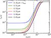 |
Fig. 7 Best-fit alignment function of silicates for the different models given by λmax. The dotted line marks the typical grain size a = 0.05 μm. The alignment function tends to shift to smaller sizes as λmax decreases. |
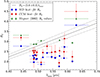 |
Fig. 8 RV–λmax plane. The red dots mark the CCM RV values as a function of λmax determinedby best-fitting the IR extinction curves with the CCM extinction law, the blue dots mark the RV values determined by fitting the WD01 model to all observations, and the green triangles mark the RV values from Wegner (2002) determined by the extrapolation method (see Table 2). The black line shows the RV relationship from Whittet & van Breda (1978) and its 1σ uncertainty. |
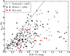 |
Fig. 9 Maximum interstellar polarization pmax vs. color excess E(B − V) of stars from Whitt et et al. (1992 black squares), Serkowski et al. (1975 black circles from), comparedto our observed sample (red circles). The straight line denotes the upper limit pmax (%) = 9.0 E(B − V) mag definedby Serkowski et al. (1975). |
7.3 pmax – E(B − V) relationship
There is no clear correlation between the maximum polarization and color excess. Figure 9 shows the Serkowski et al. (1975) and Whittet et al. (1992) sample in the pmax – E(B − V) plane compared to our sample of stars with anomalous sightlines. The scattered data in the plot shows no dependence of maximum polarization on reddening, but there is an upper limit depending on reddening (Serkowski et al. 1975) that is rarely exceeded: pmax(%) = 9.0E(B − V) mag. We calculated the mean of the ratio ⟨pmax/E(B − V)⟩ for the different samples: ⟨pmax/E(B − V)⟩ = 6.2 ± 3.8% mag−1 for the Serkowski et al. (1975) sample, ⟨pmax/E(B − V)⟩ = 4.6 ± 3.4%mag−1 for the Whittet et al. (1992) sample, and ⟨pmax/E(B − V)⟩ = 3.3 ± 2.1%mag−1 for our sample. The low ⟨pmax/E(B − V)⟩ ratio of our sample might also indicate that the silicate dust grains do not align as efficiently as the Serkowski et al. (1975) and Whittet et al. (1992) samples, but because of the small number of stars in our sample, we cannot draw such conclusions with high certainty. Another possible reason for the low ratios of pmax/E(B − V) is a small angle between the direction of the magnetic field and the line of sight, that is expected to reduce pmax/E(B − V), as discussed in previous works, for example, Hoang et al. (2014).
7.4 Which dust properties determine λmax?
For a given grain shape and dust optical constant, Eq. (16) reveals that the polarization spectrum is determined by dn∕da × fali, which is considered the size distribution of aligned grains, while the extinction (i.e., RV) in Eq. (15) is only determined by dn∕da. Thus, both a change in dn∕da and fali affect the polarization spectrum.
Our simultaneous fitting to the extinction and polarization demonstrate that both grain alignment and size distribution are required to change in order to reproduce the variation of λmax (see Figs. 6 and 7). However, the change in grain alignment is more prominent. Figure 7 shows that the alignment of small grains required to reproduce λmax = 0.45 μm is an order of magnitude higher than that required for λmax = 0.55 μm. We note that the modeling here is carried out for a constant RV. In the lines of sight where grain growth can take place, resulting in the increase of RV, we expect both grain evolution and alignment to contribute to the variation of λmax and K.
To test whether grain evolution can reproduce the observed data, we reran our simulations for the same six models by fixing the alignment function that reproduces the “standard” polarization curve with typical value λmax = 0.55 μm. The size distributions dnj ∕da was varied. We found that the variation of dn∕da can reproduce the observed data to a satisfactory level only for the cases of λmax = 0.51 – 0.55 μm, that is, λmax is not muchdifferent from the standard value. Meanwhile, the fit to the models is poor when λmax differs much from the typical value of 0.55 μm. This indicates that grain evolution alone cannot explain the wide range of λmax that is observed.
7.5 Why is K correlated to λmax?
The dependence of K on λmax appears to be an intrinsic property of the polarization. The Serkowski curve shows that a smaller K corresponds to a broader polarization profile. From the inverse modeling for a constant RV, we find that the grain alignment function becomes broader (narrower) for lower (higher) values of λmax as well as of K. This feature can be explained as follows. Each aligned grain of size a produces an individual polarization profile Cpol with the peak at λ ~ 2πa (see Fig. 1 in Hoang et al. 2013). The polarization spectrum is the superimposition/integration over all grain sizes that are aligned. When the alignment function is broader, the superposition produces a broader polarization profile, or smaller K.
7.6 Deviation of K from the standard value
To explore the dust properties underlying the deviation of K from the typical value, we performed the fit for a fixed λmax and varying k1 (in K = k1λmax + 0.01).
Figure 10 shows the best-fit models (left panel), alignment function (right panel), and size distribution (middle panel) for a fixed λmax = 0.55 μm and varying K. We find that the increase of K is produced by the decrease of large Si grains (a > 0.2 μm). At the same time, the alignment is shifted to the larger size when K increases, which is shown in Fig. 7 when λmax (and K) is increased.
7.7 Relationship between RSi and λmax
Figure 11 shows the dependence of RSi on λmax. There is a slight decrease of RSi with increasing λmax. This is straightforward because small grains are required to reproduce higher polarization in the UV when λmax decreases. The values RSi from Fig. 4 were inferred from fitting only the extinction data (Mazzei & Barbaro 2011). Thus, there is no direct relation between such inferred RSi and λmax that describes the polarization curve. It is known that a dust model that fits the extinction well may not reproduce the polarization data (e.g., dn/da ~ a−3.5 law by Mathis et al. 1977; see, e.g., Kim & Martin 1995; Draine & Fraisse 2009).
The scale difference between RSi shown in Figs. 4 and 11 arises from the different ways of modeling. In Mazzei & Barbaro (2011), to reproduce the extinction curve with low RV values, dust grains were found to be rather small (≲0.05 μm), leading to a high value of RSi. Such a dust model cannot reproduce the polarization data with standard λmax that requires aligned large grains (i.e., larger 0.1 μm). Our best-fit models that simultaneously fit extinction and polarization data provide different size distributions that have large grains, leading to smaller RSi.
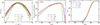 |
Fig. 10 Polarization curves (left panel), best-fit size distribution (middle panel), and best-fit alignment function (right panel) for the different values of k1, where K = k1λmax + 0.01. The value of λmax = 0.55 μm is fixed. |
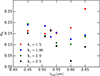 |
Fig. 11 Relative ratio of Si abundance in very small and large grain sizes vs. λmax. |
8 Summary and conclusions
We investigated the linear polarization of 17 sightlines to Galactic stars with anomalous extinction laws and low total-to-selective visual extinction ratio, RV, selected from the Mazzei & Barbaro (2011) sample, and adopted a simple dust model that can reproduce the observed sightlines with low RV values and normal polarization curves. To do this, we adopted the Weingartner & Draine (2001) dust model and a picket-fence alignment model to compute extinction and polarization curves (see Sect. 6.2.2). Our results are summarized below.
1. Galactic stars with anomalous extinction sightlines, with low RV values, show “normal” polarization curves with a mean λmax ~ 0.53 μm. This can be explained by considering that e not all dust that contributes to extinction also contributes to polarization. The polarization mainly depends on the dust grain size distribution of silicates, because grain alignment is more efficient for silicates than, for instance, for carbonaceous dust grains (Somerville et al. 1994), whereas RV is strongly dependent on carbonaceous grains too.
2. There is no significant RV –λmax relation in our sample (Fig. 8). The λmax values in our sample are higher than compared to normal stars that follow the empirical RV –λmax relationship described by Whittet & van Breda (1978), for instance.
3. Despite the low RV value, there is no similarity between the polarization curves in the investigated sample and the polarization curves observed in reddened SNe Ia with low RV values. The polarization curves are consistent with a sample of Galactic stars observed by Whittet et al. (1992) within 3σ (Fig. 2).
4. The Serkowski parameters K and λmax are correlated. However, we find a steeper slope (K = − 1.13 ± 0.34 + (4.05 ± 0.64)λmax) in our sample than in the empirical relationship found by Whittet et al. (1992), for example.
5. Simulations show that to reproduce a polarization curve with the normal λmax and low RV, there must be a population of large interstellar silicate grains of size a ≥ 0.1 μm. This is different compared to results by Mazzei & Barbaro (2008); Mazzei & Barbaro (2011), who only best-fit the extinction curves and found a lack of such large Si grains, but did find large carbonaceous grains. Moreover, variations in grain alignment and size distribution together are required to reproduce the variation in λmax for a fixed, low, RV value. However, a change in grain alignment has a greater effect.
6. By comparing the RV values of the sample here considered with those in Wegner (2002) for a subset of our stars, we find some differences that are probably due to a different spectral classification and/or luminosity class adopted to derive their extinction curves (see Sect. 7.2). The λmax value that we measure and the deviation from the empirical RV –λmax relationship may also suggest a spectral misclassification of some stars by Savage et al. (1985).
7. The K–λmax relation appears to be an intrinsic property of the polarization. Simulations show that for a fixed RV, the grain alignment function becomes narrower (broader) for a lower (higher) value of λmax and K (see Sect. 7.5).
8. An increase in Serkowski parameter K and deviation from the standard value in the K–λmax plane can be reproduced by a decreasing contribution of large Si grains (Fig. 10).
Acknowledgements
We thank the anonymous referee for useful comments that significantly improved the paper. This work is partially based on observations collected at the German-Spanish Astronomical Center, Calar Alto, jointly operated by the Max-Planck-Institut für Astronomie Heidelberg and the Instituto de Astrofisica de Andalucia (CSIC). T.H. acknowledges the support from the Basic Science Research Program through the National Research Foundation of Korea (NRF), funded by the Ministry of Education (2017R1D1A1B03035359). This work is based on observations made with ESO Telescopes at the Paranal Observatory under Program ID 094.C-0686, and partially based on observationscollected with the Copernico telescope (Asiago, Italy) of the INAF – Osservatorio Astronomico di Padova. We also thank P. Ochner for taking some observations with AFOSC in service time. Some of the data presented in this paper were obtained from the Mikulski Archive for Space Telescopes (MAST). STScI is operated by the Association of Universities for Research in Astronomy, Inc., under NASA contract NAS5-26555. Support for MAST for non-HST data is provided by the NASA Office of Space Science via grant NNX09AF08G and by other grants and contracts. ST acknowledges support from TRR33 “The Dark Universe” of the German Research Foundation.
Appendix A Standard stars
A.1 Standard stars with CAFOS
Two unpolarized standard stars were observed with CAFOS: HD 144579 (2 epochs), and HD 90508 (one epoch), and two polarized standard stars, each at two epochs: HD 154445 and HD 43384.
We used the unpolarized standard stars to investigate possible instrumental effects. The observations were binned in 200 Å bins, and the Stokes parameters, the polarization degree, and polarization angle were calculated as described in Sect. 3.3. Figure A.1 shows the derived Stokes parameters and polarization of the two unpolarized standard stars at three epochs compared to the instrumental polarization determined in Patat & Taubenberger (2011). Our measurements show consistent values between the three epochs, with average Q and U vales of 0.07 % and 0.004 %, respectively, in a wavelength range 3850–8650 Å, leading to an average polarization of P ≈ 0.10 %. The standard deviations are σQ ≈ 0.06%, σU ≈ 0.11% and σP ≈ 0.07%. The average uncertainty per 200 Å bin is ~0.03%. Our values are more consistent with zero than the values determined in Patat & Taubenberger (2011). They analyzed observations of the unpolarized star HD 14069 observed at 16 half-wave plate angles, and claimed average values of the instrumental Stokes parameters in a wavelength range above 4000 Å of ⟨Qins⟩ = 0.25 ± 0.03% and ⟨Uins⟩ = −0.13 ± 0.03%, leading to an average polarization Pins = 0.28 ± 0.03%.
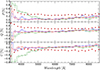 |
Fig. A.1 Unpolarized standard stars observed with CAFOS. HD 144579 was observed at two epochs, on 2015-04-30 at 00:51 UT (blue line) and 04:22 UT (green line). The red line indicates HD 90508 observed on 2015-04-29 at 21:28 UT. For comparison, the red dots indicate the instrumental polarization determined in Patat & Taubenberger (2011). |
Two polarized standard stars were observed with CAFOS, each at two epochs: HD 154445 and HD 43384. The calculated polarization spectra of HD 43384 are consistent with each other with an RMS of ~0.04%. Our Serkowski parameters (see Table C.2) are fully consistent with pmax = 3.01 ± 0.04% and λmax = 0.531 ± 0.011 μm, determined in Hsu & Breger (1982). The wavelength-dependent phase retardance variation of the half-wave plate deployed in CAFOS was quantified in Patat & Taubenberger (2011). HD 43384 has a variable (+0.6°/100 yr), and slightly wavelength dependent (+2.5 ± 1.3°/μm) polarization position angle (Hsu & Breger 1982). Therefore it is not the best standard star for HWP chromatism investigation. However, for comparison reasons, we used χ0(V) = 169.8 ± 0.7 degrees to compute the phase retardance variance and found that it is consistent with Patat & Taubenberger (2011, see Fig. A.2). The average deviation of our phase retardance variation compared to Patat & Taubenberger (2011) is ~+0.3 degrees, which is within the errors of χ0.
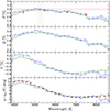 |
Fig. A.2 Polarized standard star HD 43384 observed with CAFOS at two epochs, on 2015-04-29 at 20:14 UT (green line) and 21:14 UT (blue line). The two epochs are consistent with each other with an RMS of ~0.04%. The red dashed lines in the polarization panel indicate pmax and λmax and their errors (dotted line) determined by Hsu & Breger (1982), and the red dots are their individual measurements. The red dots in the χ − χ0(V) panel indicate the phase retardance variance determined in Patat & Taubenberger (2011). |
Moreover, the two observed polarization spectra of HD 154445 are consistent with each other with an RMS of 0.07%. The average λmax = 5579 ± 11 Å and pmax = 3.64 ± 0.01% matches the literature values pmax = 3.66 ± 0.01% and λmax = 5690 ± 10Å (Wolff et al. 1996). Our average θ after the HWP chromatism correction is 89.2 ± 0.4 degree, which is similar to the literature values of θV = 88.8 ± 0.1 (Schmidt et al. 1992), θV = 90.1 ± 0.1 and θmax = 88.3 ± 0.1 degrees (Hsu & Breger 1982).
A.2 Standard stars with AFOSC
Because of lack of space in AFOSC, the Wollaston prism is inserted into the filter wheel in place of a filter for polarimetry purposes. During each observing run, it is therefore necessary to calibrate the instrument zero-point rotation angle using polarized standard stars.
We used observations of three unpolarized standard stars observed from 2015-02-09 to 2015-03-11 to investigate possible instrumental polarization of AFOSC: HD 90508 (two epochs), HD 39587 (two epochs), and HD 144579 (one epoch). They were all observed at four rotation angles of the adapter (−45, 0, 45, and 90 degrees), except for one epoch of HD 90508, which was observed at only two rotation angles (0 and 90 degrees). Figure A.3 shows the derived Stokes parameters Q and U, and the polarization for all unpolarized standard stars. The black lines indicate the epochs observed at four rotation angles, and the blue line indicates HD 90508 observed at two rotation angles. The average stokes parameters at a wavelength range above 3600 Å, excluding the range from 7500-7700Å, which is contaminated by the strong telluric 7605.0 Å O2 line, are 0.03% and −0.002% for Q and U, respectively, leading to a polarization of 0.05%, with a standard deviation of 0.05%.
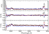 |
Fig. A.3 Unpolarized standard stars observed with AFOSC. The black lines indicate observations observed at four rotation angles, andthe blue lines indicates HD 90508 observed at two rotation angles. The red line is the average of all measurements. |
When the observations performed with the adapter rotation angles of –45 and 45 degrees are ignored and the polarization is calculated using only the adapter rotation angles of 0 and 90 degrees for all five epochs of the three standard stars, the average stokes parameters are 0.05% and −0.04% for Q and U, respectively, leading to a polarization of 0.08%, with a standard deviation of 0.10%.
HD 185395, observed on 2016-08-02, is also consistent with zero, with an average polarization above 3600 Å, excluding the range from 7500–7700 Å, of 0.08% and an RMS of 0.06%.
Three polarized standard stars were observed with AFOSC: HD 43384 (three epochs at two different runs), HD 21291 (one epoch), and HD 198478 (one epoch), all at four rotation angles of the adapter. However, because most of the science data were taken only with two rotation angles, we used only two rotation angles for consistency.
Figure A.4 shows HD 43384 at three different epochs. Although the shapes of the polarization spectra are similar, that is, λmax and K of the Serkowski fit are similar to each other, the peak polarization values, pmax, are not consistent and range from ~2.92% to ~3.19% (see Table C.3), while the literature value is pmax = 3.01 ± 0.04% (Hsu & Breger 1982).
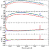 |
Fig. A.4 Polarized standard star HD 43384 observed in three different nights with AFOSC. The peak polarization values, pmax, are not fully consistent and range from ~2.92% to ~3.19%. For reference, the gray line indicates HD 43384 observed with CAFOS. |
For HD 21291, our determined peak polarization value is lower than the literature value. By fitting the Serkowski curve, we find λmax = 5166 ± 27, pmax = 2.95 ± 0.01%, while the literature values are pmax ~ 3.53 ± 0.02% and λmax = 5210 ± 30 Å (Hsu & Breger 1982).
HD 198478 was observed on 2016-08-02. Our determined peak polarization value is almost consistent with the literature value. By fitting the Serkowski curve, we find λmax = 5132 ± 42, pmax = 2.76 ± 0.01%, while the literature values are pmax ~ 2.72 ± 0.02% and λmax = 5220 ± 80 Å (Hsu & Breger 1982).
We used polarized standard stars to determine the correction of the instrument rotation angle zero-point for each of the three runs separately.
During the first run (2015-02-09), two stars were observed: HD 43384 (two epochs) and HD 21291 (one epoch). Using the
literature values of χV = 169.8 ± 0.7 degrees for HD 43384, and χV = 116.6 ± 0.2 degrees for HD 21291, we calculated a weighted average of the offset Δ θV = 136.4 ± 0.3 degrees.
During the second run (2015-03-09), HD 43384 was observed at one epoch, from which we calculated the instrument rotation angle zero-point offset ΔθV = 134.0 ± 0.8 degrees.
Finally, from HD 198478 observed during the third run (2016-08-02), we calculated Δ θV = 138.3 ± 0.4 degrees.
Appendix B Serkowski fit to SNe Ia
We determined the Serkowski parameters of the sodium sample in Zelaya et al. (2017) by fitting Eq. (1) to the data shown in their Fig. 1. The polarized lines were excluded from the wavelength range. The results are given in Table B.1.
Serkowski paramaters of the SNe Ia sodium-sample (Zelaya et al. 2017).
Appendix C Individual observations
Individual epochs with FORS2.
Individual epochs with CAFOS
Individual epochs with AFOSC
References
- Altavilla, G., Fiorentino, G., Marconi, M., et al. 2004, MNRAS, 349, 1344 [NASA ADS] [CrossRef] [Google Scholar]
- Anderson, C. M., Weitenbeck, A. J., Code, A. D., et al. 1996, AJ, 112, 2726 [NASA ADS] [CrossRef] [Google Scholar]
- Andersson, B.-G., Lazarian, A., & Vaillancourt, J. E. 2015, ARA&A, 53, 501 [NASA ADS] [CrossRef] [Google Scholar]
- Bagnulo, S., Cox, N. L. J., Cikota, A., et al. 2017, A&A, 608, A146 [NASA ADS] [CrossRef] [EDP Sciences] [Google Scholar]
- Cardelli, J. A., Clayton, G. C., & Mathis, J. S. 1989, ApJ, 345, 245 [NASA ADS] [CrossRef] [Google Scholar]
- Chiar, J. E., Adamson, A. J., Whittet, D. C. B., et al. 2006, ApJ, 651, 268 [CrossRef] [Google Scholar]
- Cikota, A., Deustua, S., & Marleau, F. 2016, ApJ, 819, 152 [NASA ADS] [CrossRef] [Google Scholar]
- Cikota, A., Patat, F., Cikota, S., & Faran, T. 2017a, MNRAS, 464, 4146 [NASA ADS] [CrossRef] [Google Scholar]
- Cikota, A., Patat, F., Cikota, S., Spyromilio, J., & Rau, G. 2017b, MNRAS, 471, 2111 [NASA ADS] [Google Scholar]
- Clayton, G. C., & Mathis, J. S. 1988, ApJ, 327, 911 [NASA ADS] [CrossRef] [Google Scholar]
- Clayton, G. C., Wolff, M. J., Allen, R. G., & Lupie, O. L. 1995, ApJ, 445, 947 [NASA ADS] [CrossRef] [Google Scholar]
- Clayton, G. C., Wolff, M. J., Sofia, U. J., Gordon, K. D., & Misselt, K. A. 2003, ApJ, 588, 871 [NASA ADS] [CrossRef] [Google Scholar]
- Conley, A., Carlberg, R. G., Guy, J., et al. 2007, ApJ, 664, L13 [NASA ADS] [CrossRef] [Google Scholar]
- Coyne, G. V., Gehrels, T., & Serkowski, K. 1974, AJ, 79, 581 [NASA ADS] [CrossRef] [Google Scholar]
- Draine, B. T. 2003, ARA&A, 41, 241 [NASA ADS] [CrossRef] [Google Scholar]
- Draine, B. T., & Allaf-Akbari, K. 2006, ApJ, 652, 1318 [NASA ADS] [CrossRef] [Google Scholar]
- Draine, B. T., & Fraisse, A. A. 2009, ApJ, 696, 1 [NASA ADS] [CrossRef] [Google Scholar]
- Draine, B. T., & Li, A. 2007, ApJ, 657, 810 [NASA ADS] [CrossRef] [Google Scholar]
- ESO 2015, FORS2 User Manual, issue 96.0, VLT-MAN-ESO-13100-1543 (European Southern Observatory) [Google Scholar]
- Fitzpatrick, E. L. 1999, PASP, 111, 63 [NASA ADS] [CrossRef] [Google Scholar]
- Fitzpatrick, E. L., & Massa, D. 2007, ApJ, 663, 320 [NASA ADS] [CrossRef] [EDP Sciences] [Google Scholar]
- Folatelli, G., Phillips, M. M., Burns, C. R., et al. 2010, AJ, 139, 120 [NASA ADS] [CrossRef] [Google Scholar]
- Foley, R. J., Fox, O. D., McCully, C., et al. 2014, MNRAS, 443, 2887 [NASA ADS] [CrossRef] [Google Scholar]
- Giridhar, S., & Arellano Ferro, A. 2005, A&A, 443, 297 [NASA ADS] [CrossRef] [EDP Sciences] [Google Scholar]
- Goobar, A. 2008, ApJ, 686, L103 [NASA ADS] [CrossRef] [Google Scholar]
- Hicken, M., Wood-Vasey, W. M., Blondin, S., et al. 2009, ApJ, 700, 1097 [NASA ADS] [CrossRef] [Google Scholar]
- Hoang, T. 2017, ApJ, 836, 13 [NASA ADS] [CrossRef] [Google Scholar]
- Hoang, T., & Lazarian, A. 2016, ApJ, 831, 159 [NASA ADS] [CrossRef] [Google Scholar]
- Hoang, T., Lazarian, A., & Martin, P. G. 2013, ApJ, 779, 152 [NASA ADS] [CrossRef] [Google Scholar]
- Hoang, T., Lazarian, A., & Martin, P. G. 2014, ApJ, 790, 6 [NASA ADS] [CrossRef] [Google Scholar]
- Hong, S. S., & Greenberg, J. M. 1980, A&A, 88, 194 [NASA ADS] [Google Scholar]
- Hsu, J.-C., & Breger, M. 1982, ApJ, 262, 732 [NASA ADS] [CrossRef] [Google Scholar]
- Johnson, J. J., & Jones, T. J. 1991, AJ, 101, 1735 [NASA ADS] [CrossRef] [Google Scholar]
- Kessler, R., Becker, A. C., Cinabro, D., et al. 2009, ApJS, 185, 32 [NASA ADS] [CrossRef] [Google Scholar]
- Kim, S.-H., & Martin, P. G. 1995, ApJ, 444, 293 [NASA ADS] [CrossRef] [Google Scholar]
- Lampeitl, H., Smith, M., Nichol, R. C., et al. 2010, ApJ, 722, 566 [NASA ADS] [CrossRef] [Google Scholar]
- Lazarian, A., Andersson, B.-G., & Hoang, T. 2015, in Polarimetry of stars and planetary systems, eds. L. Kolokolova, J. Hough, & A.-C. Levasseur-Regourd (Cambridge, UK: Cambridge Univ. Press), 81 [Google Scholar]
- Lü, G., Zhu, C., & Podsiadlowski, P. 2013, ApJ, 768, 193 [NASA ADS] [CrossRef] [Google Scholar]
- Mandel, K. S., Narayan, G., & Kirshner, R. P. 2011, ApJ, 731, 120 [NASA ADS] [CrossRef] [Google Scholar]
- Martin, P. G., Clayton, G. C., & Wolff, M. J. 1999, ApJ, 510, 905 [NASA ADS] [CrossRef] [Google Scholar]
- Mathis, J. S., Rumpl, W., & Nordsieck, K. H. 1977, ApJ, 217, 425 [NASA ADS] [CrossRef] [Google Scholar]
- Mazzei, P., & Barbaro, G. 2008, MNRAS, 390, 706 [NASA ADS] [CrossRef] [Google Scholar]
- Mazzei, P., & Barbaro, G. 2011, A&A, 527, A34 [NASA ADS] [CrossRef] [EDP Sciences] [Google Scholar]
- Nobili, S., & Goobar, A. 2008, A&A, 487, 19 [NASA ADS] [CrossRef] [EDP Sciences] [Google Scholar]
- Oliva, E. 1997, A&AS, 123, 589 [NASA ADS] [CrossRef] [EDP Sciences] [Google Scholar]
- Oppenheimer, B. D., Bieging, J. H., Schmidt, G. D., et al. 2005, ApJ, 624, 957 [NASA ADS] [CrossRef] [Google Scholar]
- Patat, F., & Romaniello, M. 2006, PASP, 118, 146 [NASA ADS] [CrossRef] [Google Scholar]
- Patat, F., & Taubenberger, S. 2011, A&A, 529, A57 [NASA ADS] [CrossRef] [EDP Sciences] [Google Scholar]
- Patat, F., Maund, J. R., Benetti, S., et al. 2010, A&A, 510, A108 [NASA ADS] [CrossRef] [EDP Sciences] [Google Scholar]
- Patat, F., Taubenberger, S., Cox, N. L. J., et al. 2015, A&A, 577, A53 [NASA ADS] [CrossRef] [EDP Sciences] [Google Scholar]
- Phillips, M. M., Lira, P., Suntzeff, N. B., et al. 1999, AJ, 118, 1766 [NASA ADS] [CrossRef] [Google Scholar]
- Phillips, M. M., Simon, J. D., Morrell, N., et al. 2013, ApJ, 779, 38 [NASA ADS] [CrossRef] [Google Scholar]
- Pourbaix, D., Tokovinin, A. A., Batten, A. H., et al. 2004, A&A, 424, 727 [NASA ADS] [CrossRef] [EDP Sciences] [Google Scholar]
- Reindl, B., Tammann, G. A., Sandage, A., & Saha, A. 2005, ApJ, 624, 532 [NASA ADS] [CrossRef] [Google Scholar]
- Riess, A. G., Press, W. H., & Kirshner, R. P. 1996, ApJ, 473, 588 [NASA ADS] [CrossRef] [Google Scholar]
- Savage, B. D., Massa, D., Meade, M., & Wesselius, P. R. 1985, ApJS, 59, 397 [NASA ADS] [CrossRef] [Google Scholar]
- Schmidt, G. D., Elston, R., & Lupie, O. L. 1992, AJ, 104, 1563 [NASA ADS] [CrossRef] [Google Scholar]
- Serkowski, K., Mathewson, D. S., & Ford, V. L. 1975, ApJ, 196, 261 [NASA ADS] [CrossRef] [Google Scholar]
- Somerville, W. B., Allen, R. G., Carnochan, D. J., et al. 1994, ApJ, 427, L47 [NASA ADS] [CrossRef] [Google Scholar]
- Trujillo-Bueno, J., Moreno-Insertis, F., & Sanchez Martinez F. 2002, Astrophysical Spectropolarimetry (Cambridge, UK: Cambridge University Press), 368 [Google Scholar]
- Voshchinnikov, N. V. 2012, J. Quant. Spectr. Rad. Transf., 113, 2334 [Google Scholar]
- Wang, L. 2005, ApJ, 635, L33 [NASA ADS] [CrossRef] [Google Scholar]
- Wang, L., & Wheeler, J. C. 2008, ARA&A, 46, 433 [NASA ADS] [CrossRef] [Google Scholar]
- Wang, X., Wang, L., Pain, R., Zhou, X., & Li, Z. 2006, ApJ, 645, 488 [NASA ADS] [CrossRef] [Google Scholar]
- Wang, X., Li, W., Filippenko, A. V., et al. 2008, ApJ, 677, 1060 [NASA ADS] [CrossRef] [Google Scholar]
- Wegner, W. 2002, Baltic Astron., 11, 1 [Google Scholar]
- Weingartner, J. C., & Draine, B. T. 2001, ApJ, 548, 296 [NASA ADS] [CrossRef] [Google Scholar]
- Wesselius, P. R., van Duinen, R. J., de Jonge, A. R. W., et al. 1982, A&AS, 49, 427 [NASA ADS] [Google Scholar]
- Whittet, D. C. B., & van Breda I. G. 1978, A&A, 66, 57 [NASA ADS] [Google Scholar]
- Whittet, D. C. B., Martin, P. G., Hough, J. H., et al. 1992, ApJ, 386, 562 [NASA ADS] [CrossRef] [Google Scholar]
- Whittet, D. C. B., Gerakines, P. A., Carkner, A. L., et al. 1994, MNRAS, 268, 1 [NASA ADS] [CrossRef] [Google Scholar]
- Whittet, D. C. B., Gerakines, P. A., Hough, J. H., & Shenoy, S. S. 2001, ApJ, 547, 872 [NASA ADS] [CrossRef] [Google Scholar]
- Wilking, B. A., Lebofsky, M. J., Kemp, J. C., Martin, P. G., & Rieke, G. H. 1980, ApJ, 235, 905 [NASA ADS] [CrossRef] [Google Scholar]
- Wilking, B. A., Lebofsky, M. J., & Rieke, G. H. 1982, AJ, 87, 695 [NASA ADS] [CrossRef] [Google Scholar]
- Wolff, M. J., Nordsieck, K. H., & Nook, M. A. 1996, AJ, 111, 856 [NASA ADS] [CrossRef] [Google Scholar]
- Yang, Y., Wang, L., Baade, D., et al. 2017, ApJ, 834, 60 [NASA ADS] [CrossRef] [Google Scholar]
- Zelaya, P., Clocchiatti, A., Baade, D., et al. 2017, ApJ, 836, 88 [NASA ADS] [CrossRef] [Google Scholar]
All Tables
All Figures
|
Fig. 1 Weighted averages of observed polarization curves for all science targets, derived with different instruments. The red circles show observations performed with FORS2, blue triangles with CAFOS, green squares with AFOSC, and left-pointingpurple triangles with HPOL. The full lines denote the Serkowski fits, as parametrized in Table 3. |
| In the text | |
|
Fig. 2 Stars with anomalous extinction sightlines in the λmax-K plane. Blue shows stars with anomalous sightlines observed with FORS2 (circles), CAHA (right pointing triangles), AFOSC (squared), and HPOL (left-pointing triangles). The solid blue line represents the linear best fit to the sample, and its 1σ deviation (dotted). The dashed black line traces the Whittet et al. (1992) relation and its 3σ uncertainty(dotted). For comparison, a sample of SNe Ia from Patat et al. (2015) and Zelaya et al. (2017; see Appendix B) are marked with stars and red contours, which indicate the 10 and 20 σ confidence levels for SN 2008fp and SN 2014J. |
| In the text | |
|
Fig. 3 Comparison of our sample of stars with anomalous extinction sightlines (blue symbols) to the Whittet et al. (1992) sample (gray squares) and the LIPS sample (Bagnulo et al. 2017, red circles). The gray ellipses represent 1–5σ confidence levels for the Whittet et al. (1992) sample. The dashed black line traces the Whittet et al. (1992) relation and its 1σ uncertainty (dotted). |
| In the text | |
|
Fig. 4 RSi–λmax relationship. The red dots represent stars observed with FORS2, AFOSC, and CAFOS, and the black dots show seven additional measurements from HPOL or from the literature. The red dashed line is the linear least-squares fit to the red dots, and the black solid line is the linear least-squares fit to all data. |
| In the text | |
|
Fig. 5 Left panel: best-fit models vs. generated (i.e., constructed) polarization curves for six different models described by λmax. Right panel: best-fit models vs. generated extinction curves with a low RV = 2.5. Filled circles show the generated data, and solid lines show our best-fit models. |
| In the text | |
|
Fig. 6 Best-fit grain size distribution for silicate (left panel) and carbonaceous grains (right panel). Six different models described by λmax are considered. Large silicate grains of size a ≥ 0.1μm are present to reproduce normal λmax. |
| In the text | |
|
Fig. 7 Best-fit alignment function of silicates for the different models given by λmax. The dotted line marks the typical grain size a = 0.05 μm. The alignment function tends to shift to smaller sizes as λmax decreases. |
| In the text | |
|
Fig. 8 RV–λmax plane. The red dots mark the CCM RV values as a function of λmax determinedby best-fitting the IR extinction curves with the CCM extinction law, the blue dots mark the RV values determined by fitting the WD01 model to all observations, and the green triangles mark the RV values from Wegner (2002) determined by the extrapolation method (see Table 2). The black line shows the RV relationship from Whittet & van Breda (1978) and its 1σ uncertainty. |
| In the text | |
|
Fig. 9 Maximum interstellar polarization pmax vs. color excess E(B − V) of stars from Whitt et et al. (1992 black squares), Serkowski et al. (1975 black circles from), comparedto our observed sample (red circles). The straight line denotes the upper limit pmax (%) = 9.0 E(B − V) mag definedby Serkowski et al. (1975). |
| In the text | |
|
Fig. 10 Polarization curves (left panel), best-fit size distribution (middle panel), and best-fit alignment function (right panel) for the different values of k1, where K = k1λmax + 0.01. The value of λmax = 0.55 μm is fixed. |
| In the text | |
|
Fig. 11 Relative ratio of Si abundance in very small and large grain sizes vs. λmax. |
| In the text | |
|
Fig. A.1 Unpolarized standard stars observed with CAFOS. HD 144579 was observed at two epochs, on 2015-04-30 at 00:51 UT (blue line) and 04:22 UT (green line). The red line indicates HD 90508 observed on 2015-04-29 at 21:28 UT. For comparison, the red dots indicate the instrumental polarization determined in Patat & Taubenberger (2011). |
| In the text | |
|
Fig. A.2 Polarized standard star HD 43384 observed with CAFOS at two epochs, on 2015-04-29 at 20:14 UT (green line) and 21:14 UT (blue line). The two epochs are consistent with each other with an RMS of ~0.04%. The red dashed lines in the polarization panel indicate pmax and λmax and their errors (dotted line) determined by Hsu & Breger (1982), and the red dots are their individual measurements. The red dots in the χ − χ0(V) panel indicate the phase retardance variance determined in Patat & Taubenberger (2011). |
| In the text | |
|
Fig. A.3 Unpolarized standard stars observed with AFOSC. The black lines indicate observations observed at four rotation angles, andthe blue lines indicates HD 90508 observed at two rotation angles. The red line is the average of all measurements. |
| In the text | |
|
Fig. A.4 Polarized standard star HD 43384 observed in three different nights with AFOSC. The peak polarization values, pmax, are not fully consistent and range from ~2.92% to ~3.19%. For reference, the gray line indicates HD 43384 observed with CAFOS. |
| In the text | |
Current usage metrics show cumulative count of Article Views (full-text article views including HTML views, PDF and ePub downloads, according to the available data) and Abstracts Views on Vision4Press platform.
Data correspond to usage on the plateform after 2015. The current usage metrics is available 48-96 hours after online publication and is updated daily on week days.
Initial download of the metrics may take a while.