| Issue |
A&A
Volume 614, June 2018
|
|
|---|---|---|
| Article Number | A17 | |
| Number of page(s) | 13 | |
| Section | Stellar structure and evolution | |
| DOI | https://doi.org/10.1051/0004-6361/201732065 | |
| Published online | 06 June 2018 | |
Modelling the carbon AGB star R Sculptoris
Constraining the dust properties in the detached shell based on far-infrared and sub-millimeter observations★
1
Department for Astrophysics, University of Vienna,
Türkenschanzstrasse 17,
1180
Vienna,
Austria
e-mail: This email address is being protected from spambots. You need JavaScript enabled to view it.
2
Department of Space, Earth and Environment, Chalmers University of Technology,
43992
Onsala,
Sweden
Received:
9
October
2017
Accepted:
25
January
2018
Abstract
Context. On the asymptotic giant branch (AGB), Sun-like stars lose a large portion of their mass in an intensive wind and enrich the surrounding interstellar medium with nuclear processed stellar material in the form of molecular gas and dust. For a number of carbon-rich AGB stars, thin detached shells of gas and dust have been observed. These shells are formed during brief periods of increased mass loss and expansion velocity during a thermal pulse, and open up the possibility to study the mass-loss history of thermally pulsing AGB stars.
Aims. We study the properties of dust grains in the detached shell around the carbon AGB star R Scl and aim to quantify the influence of the dust grain properties on the shape of the spectral energy distribution (SED) and the derived dust shell mass.
Methods. We modelled the SED of the circumstellar dust emission and compared the models to observations, including new observations of Herschel/PACS and SPIRE (infrared) and APEX/LABOCA (sub-millimeter). We derived present-day mass-loss rates and detached shell masses for a variation of dust grain properties (opacities, chemical composition, grain size, and grain geometry) to quantify the influence of changing dust properties to the derived shell mass.
Results. The best-fitting mass-loss parameters are a present-day dust mass-loss rate of 2 × 10⁻¹⁰ M⊙ yr−1 and a detached shell dust mass of (2.9 ± 0.3) × 10−5 M⊙. Compared to similar studies, the uncertainty on the dust mass is reduced by a factor of 4. We find that the size of the grains dominates the shape of the SED, while the estimated dust shell mass is most strongly affected by the geometry of the dust grains. Additionally, we find a significant sub-millimeter excess that cannot be reproduced by any of the models, but is most likely not of thermal origin.
Key words: stars: AGB and post-AGB / stars: evolution / stars: carbon / stars: mass-loss / stars: late-type
Herschel is an ESA space observatory with science instruments provided by European-led Principal Investigator consortia and with important participation from NASA.
© ESO 2018
1 Introduction
During the late stages of stellar evolution, stars with low to intermediate mass (~0.8 to 8 M⊙) develop strong stellar winds as they evolve along the asymptotic giant branch (AGB). On the AGB they consist of a carbon-oxygen core surrounded by hydrogen- and helium-burning shells and a deep convective envelope. The average mass-loss rates range roughly from 10−7 to 10−5M⊙ yr−1, but large variations in the mass-loss rates and a non-linear mass-loss evolution are seen throughout different evolutionary stages on the AGB (e.g. review by Habing 1996).
The chemistry in the outer layers of AGB stars changes during its evolution due to nuclear burning in shells around the stellar core and dredge-up events of nuclear processed elements to the stellar surface during thermal pulses (TPs). This alters the chemical composition of the stellar atmosphere, and consequently also of the molecular gas and dust species found in the circumstellar envelopes (CSEs). These molecules and dust grains can be formed in regions of low temperatures and high densities in the outer CSE.
Through their mass loss, AGB stars provide up to 80% of dust in the Milky Way and contribute to the chemical evolution of local galaxies (Forestini & Charbonnel 1997; Herwig & Austin 2004; Schneider et al. 2014), while their contribution to the total dust budget is less certain in the early Universe (Mancini et al. 2015). The origin of dust grains and the associated dust grain properties are important for understanding their chemical composition, the lifetime of dust grains in the interstellar radiation field, and their role in star and planet formation. In particular, the grain size and geometry strongly affect the survival of dust grains in the interstellar medium (ISM) and star formation processes, and the possibility for the grains to carry organic molecules into proto-planetary disks.
During a TP the luminosity and radius of the star increase for a few hundred years. This leads to an increase in the mass-loss rate and expansion velocity of the stellar wind, before subsequently declining to pre-pulse values (e.g. Steffen & Schönberner 2000; Mattsson et al. 2007). A consequence of this change in mass-loss properties is the formation of detached shells – geometrically thin shells of dust and gas that expand away from the star (e.g. Olofsson et al. 1988, 1990). Detached shells offer a direct opportunity to study the evolution of the star and stellar mass-loss throughout the TP-cycle, and hence provide the possibility to constrain one of the fundamental processes in late stellar evolution.
The target of this publication is R Scl, a well-studied carbon-rich AGB star with a semi-regular pulsation period of ~370 days (Knapp et al. 2003). Models by Sacuto et al. (2011) and Wittkowski et al. (2017) require a luminosity of 7000 L⊙ and effective temperatures of 2700 and 2640 ± 80 K for distances of 350 and 370 pc, respectively. We adopt a distance of 370 pc, which is derived from the P–L relationshipfor semi-regular variables (with an uncertainty of 370 pc, Knapp et al. 2003), which is in agreement with a recent study on an independent, more accurate distance estimate of Maercker et al. (2018).
R Scl is known to be surrounded by a detached shell, believed to have been formed during a TP event, and is seen in molecular gas (e.g. Olofsson et al. 1990, 1996; Maercker et al. 2012) as well as co-spatial dust emission (e.g. González Delgado et al. 2001, 2003; Olofsson et al. 2010; Maercker et al. 2014). Additionally, a spiral structure, which is associated with wind-binary interaction, connects the present-day wind with the detached shell (Maercker et al. 2012). These high-resolution observations of the molecular CO gas, carried out with the Atacama Large sub-Millimeter Array (ALMA)1, have given good constraints on the spatial density distribution of the gas, and constrained the evolution of the gas mass-loss rate during and after the most recent thermal pulse (Maercker et al. 2012, 2016). Based on the expansion velocity of the CO shell and the distance of 370 pc, the detached shell was created 2300 years ago (Maercker et al. 2016). Observations of the polarised dust-scattered stellar light at optical wavelengths have provided detailed information on the distribution of dust in the shell and give an average radius of 19.5′′± 0.5′′ and (FWHM) width of 2′′± 1′′ (González Delgado et al. 2003; Maercker et al. 2014). Nonetheless, the scattered-light observations do not provide information on the velocity and temperature of the dust, and only with difficulty allow determining the total dust mass or the grain properties. To date, modelling of the thermal dust emission from the detached shell around R Scl is limited to models of the spectral energy distribution (SED) from optical to far-infrared (FIR) wavelengths (Schöier et al. 2005). However, this previous study did not consider the spatial constraints on the dust shell provided by the scattered-light observations, and was not aimed at constraining the dust properties in detail.
In this paper we present new radiative transfer models of the thermal dust emission towards R Scl. The primary goals of this study are to derive the dust mass in the detached shell around R Scl and to determine the dust properties. We attempt to describe the dependency of the derived dust-shell parameters on implemented opacities, chemical grain composition, grain sizes and grain geometries. We model the SED and include FIR observations with Herschel PACS (Poglitsch et al. 2010) and SPIRE (Griffin et al. 2010). In addition, we present a map of the dust emission at sub-millimeter wavelengths (870 μm) observed with LABOCA (Siringo et al. 2009) on APEX2. The spatial resolution of the LABOCA observations resolves the shell around R Scl. The new observations and models allow us to study the dust properties in the circumstellar environment around R Scl across the entire wavelength range from optical to sub-millimeter, and in particular allow us to constrain the properties of the dust in the cold shell around the star.
In Sect. 2 we present a summary of new and archive observations as well as previous modelling results. Our approach of the dust radiative transfer modelling is described in Sect. 3, and our results are summarised and discussed in Sect. 4. A conclusion of our findings is given in Sect. 5.
2 Observations of R Scl
2.1 Spectral energy distribution towards R Scl
Following the work done previously by Schöier et al. (2005), we used archival photometric observations to create the SED from 0.44 to 100 μm. We additionally included Herschel/PACS photometry at 70 and 160 μm, and Herschel/SPIRE photometry at 250, 350 and 500 μm (Obs. IDs 1342213264, 1342213265 and 1342188657) observed in the Mass-loss of Evolved StarS (MESS) program (Groenewegen et al. 2011; Cox et al. 2012). We added new observations of the continuum emission towards R Scl at sub-millimeter wavelengths at 870 μm with APEX/LABOCA (see Sect. 2.3). Additionally, ALMA continuum observations between 887 and 2779 μm were included (see next section). A list of the used SED data points is given in Table 1, and the full SED is plotted in Fig. 1.
Observations of the spectral energy distribution.
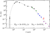 |
Fig. 1 SED of R Scl. Black: points used in Schöier et al. (2005); green: Herschel/PACS; blue: Herschel/SPIRE; red: LABOCA; purple: ALMA. Plotted with the grey dashed line is the overall best-fit model of the star, present-day wind, and detached shell (see Sect. 4.1). |
2.2 Continuum observations from ALMA
The ALMA observations were taken during ALMA Early Science in Cycle 0 (ADS/JAO.ALMA#2011.0.00131.S), with 16 antennas in the main array in ALMA Bands 3, 6, and 7 (for more details on the observations, we refer to Maercker et al. 2012, 2016). The aim of the observations was to observe the CO emission from the detached shell and CSE. In thecontinuum, the ALMA observations only allow detecting the stellar emission (possibly with a small contributionfrom the very recent mass loss) – the detached shell is not visible with the achieved sensitivity and resolution. This is confirmed by the models of the stellar contribution to the SED (see Sect. 3.3). The ALMA observations are hence not used for constraining our radiative transfer models of the star, shell, or present-day mass loss, but are merely used to verify the spatial origin of the LABOCA observations (see next section).
2.3 APEX/LABOCA observations
The Large Bolometer Camera (LABOCA) on APEX is a 295-channel bolometer array that observes the sky at 870 μm with a bandwidth of 150 μm (Siringo et al. 2009). The beam size of APEX at this wavelength is 18.6′′.
We retrieved archival data of R Scl observed with LABOCA in August, October, and November 2007 (Program ID: O-079. F-9309A). The total observing time (on- and off-source) was 10.8 h. The data were re-reduced using CRUSH (Kovács 2008). The final map has an rms noise of 4.5 mJy, and the peak flux corresponds to 0.1 Jy beam−1 (Fig. 2, top). The extended emission is detected at a signal-to-noise ratio of approximately 10.
Since the ALMA observations only show the stellar emission, we used them to separate the stellar from the circumstellar flux observed in the LABOCA data. We convolved the ALMA Band 7 observations with the LABOCA beam, and subtracted the emission from the LABOCA map. The resulting map shows the remaining circumstellar emission (Fig. 2, middle), which no longer includes any stellar emission. The bottom panel of Fig. 2 shows the circumstellar emission subtracted by a thin shell corresponding to the detached shell around R Scl, showing that the circumstellar emission indeed is consistent with a shell with a radius of ~19′′ and a width of ~2′′ around R Scl. The residual emission seen in the bottom panel of Fig. 2 can be attributed to asymmetries compared to the spherically symmetric shell that was subtracted.
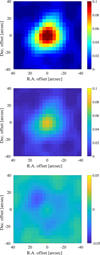 |
Fig. 2 Top: LABOCA observations towards R Scl. The colour scale is given in Jy beam−1. Middle: LABOCA map with the stellar SED (retrieved from the ALMA continuum observations convolved by the LABOCA beam) subtracted. Bottom: residual map after subtracting the stellar SED and a spherical detached shell with a radius of 18′′.5 and width of 2′′. The structures in the residual map are due to asymmetric emission from the shell, consistent with scattered-light observations. |
3 Dust radiative transfer modelling
3.1 SED models with MCMax
We used theMonte Carlo dust radiative transfer code MCMax (Min et al. 2009) to model the circumstellar dust emission of R Scl. The Monte Carlo method of radiative transfer calculates the absorption, re-emission, and scattering processes for a large number of individual photon packages, which are moving through the modelled medium described by a specific density and opacity at each grid cell. After all photon packages have escaped the grid, the temperature and frequency structure at each grid cell is the output of the model. The resulting observables are the SED, images of the emission, polarisation maps, and visibilities. The required input for such models are the properties of the illuminating source, the density profile, and the opacity of the surrounding medium.
Although MCMax is capable of 3D (axisymmetric) radiative transfer modelling, we employed only a 1D radial density profile to describe the spherically symmetric detached shell and present-day mass loss of R Scl. This creates a homogeneous envelope and shell aroundthe star. Although small-scale structure and clumpiness is observed around R Scl (in the form of a spiral imprinted on the CSE and clumpy structure in the shell; Maercker et al. 2012, 2016), in the case of optically thin dust emission, the dominating parameter affecting the dust emission is the radial distance to the star and the intrinsic properties of the individual dust grains.
3.2 General assumptions and modelling strategy
We modelled and discuss the circumstellar environment of R Scl with respect to three thermal components that contribute to the observed SED: the star itself as dominating radiation source, surrounded by the present-day wind or CSE (starting at the dust condensation radius), and the thin, spherical dust shell located at ≈19′′ from the star. We assumed that the dust emission is optically thin. This allowed us to model the three different contributions to the SED separately, adding the flux from the star, the present-day wind, and the shell to obtain the full SED to be compared to observations. We limited the outer radius of the dust density distribution to 10 000 AU (at 370 pc the shell has a physical radius of ≈7200 AU), while the inner radius was automatically calculated by MCMax through dust destruction of all particles with a temperature above the given dust condensation temperature (which is considered to be equivalent to the dust destruction temperature).
The focus of this modelling strategy is the analysis of the properties of the shell, and in particular, exploring the constraints set by the FIR and sub-millimeter observations. We therefore did not model the stellar SED and present-day wind in (much) detail, other than reproducing the effective flux created inside the shell.
3.3 Stellar parameters and contribution
We treated the star as a black body with an effective temperature Teff,⋆ and luminosity L⋆, located at a distance D. The emitted flux thus follows the Planck law for black-body radiation, and for AGB stars with low effective temperatures, the emission will peak around a few μm – dominating the SED in that wavelength range. The stellar parameters of R Scl have been derived with several different approaches and have been extracted from various modelling attempts (as described in the introduction). To be consistent within our modelling approach, we calculated a small grid of black bodies with varying Teff,⋆ and L⋆ to determine the best-fitting parameters to our observational data, shorter than 4 μm (main stellar contribution). The best-fitting parameters are Teff,⋆ = 2250 K and L⋆ = 7000 L⊙ for a distance of D = 370 pc. As presented in the introduction, these values are in general agreement with earlier publications (e.g. Schöier et al. 2005; Sacuto et al. 2011; Wittkowski et al. 2017), although our best-fitting effective temperature is lower than in all previous models. We emphasise that this is most likely because we included optical data in our SED fit. In general, the difference in temperature is not significant for our further analysis, since we did not attempt to separate the stellar and present-day wind contribution perfectly, but concentrated on modelling the shell emission. These parameters were used as input in all following models of the present-day wind and shell, and were not changed. Figure 3 shows the model grid of calculated black bodies for determining the best-fitting stellar parameters. It is evident that the ALMA observations do not represent any detached-shell contribution but are reproduced by the stellar contribution alone.
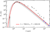 |
Fig. 3 Model grid of black bodies with different luminosities and effective temperatures (grey lines). The best-fitting model is shown as a red line. All SED data points below 4 μm are used for χ-square fitting (black dots); data points with wavelengths longer than that are plotted in grey; the ALMA data points are shown in blue for reference. |
3.4 Present-day wind description
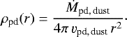
The present-day wind is described as the “most recent” mass-loss process, usually attributed to a smooth, spherical stellar wind, expanding outwards from the dust-condensation radius at a few stellar radii, with a constant and low to intermediate mass-loss rate Ṁ pd, dust and expansion velocity vpd, dust. The associated 1D radial density profile of thepresent-day wind, ρpd(r), can be described by a power law:
 (1)
(1)
The dust expansion velocity, vpd, dust, cannot be directly measured by observations. Gas expansion velocities can be measured with high accuracy, however, and assuming full coupling between the dust and gas (i.e. zero drift velocity), we can obtain a first-order estimate of the dust velocity. A non-zero drift velocity will change our model output by scaling the calculated dust mass-loss rates. The presented dust mass-loss rates are therefore lower limits, concerning a possibly higher dust velocity than currently used.
We notethat for the shell, the dust and gas seem to coincide almost perfectly (Maercker et al. 2014), indicating that the drift-velocity is indeed close to zero. However, this does not have to be true throughout the evolution of the shell and wind, or for all components of the circumstellar dust distribution.
Observations of the molecular gas indicate that the mass-loss rate has not been constant since the last thermal pulse, but rather has been continuously declining in both rate and expansion velocity (Maercker et al. 2012, 2016). The density distribution of the CSE created in that case would not follow the r−2 dependence of Eq. (1). However, we are primarily interested in the properties of the dust in the shell, which are constrained by observations at wavelengths >20 μm, and the details of the dust distribution at radii smaller than the shell radius are not critical, as long as they provide the correct radiation field. More importantly, the spatial resolution of the current observations are not sufficient to constrain the distribution of the dust inside the shell. The determined value for the present-day mass-loss rate should therefore be interpreted with some care.
3.5 Detached-shell description
The spatial extent of the detached shell of dust around R Scl (in angular scale) is well defined through the observations in dust scattered stellar light (Maercker et al. 2014, and references therein), and appears to be the same as for the shell of gas in high-resolution observations with ALMA (Maercker et al. 2012, 2016). Assuming that the distance to R Scl is known, a linear radius and thickness of the shell can be derived. We assumed a smooth, Gaussian density distribution for the shell with the following radial density profile:
 (2)
(2)
where σshell is the standard deviation of the Gaussian shell, related to the FWHM of the shell. ρ0 is the peak density in the detached shell, which we derived by dividing Mshell, dust, the mass contained within ± 5σ of the Gaussian shell, by the corresponding volume, V shell, of the Gaussian shell:
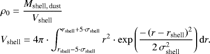
Therefore, the radial density profile of the shell can be directly defined by the input of a specific dust shell mass, Mshell, dust, which is the only variable to define.
3.6 Dust properties
The emission from the dust grains is determined by the properties of the individual dust grains. The dust parameters such as grain size, grain density, grain geometry (e.g. solid spheres, distribution of hollow spheres), chemical composition, and condensation temperature determine the absorption and scattering efficiency of the material, and are reflected in the form of the individual opacity tables. These are necessary input for the modelling code. Such opacity tables are based on laboratory measurements of the real and imaginary part of the complex refractive index, which are provided in various databases (e.g. the Jena database3), and were used to calculate the frequency dependent absorption opacity  and the scattering opacity
  based on the assumed grain model. With the dust properties and frequency-dependent opacity tables, the radiative transfer equations were solved for each absorption, scattering or emission event for each photon package, sent through the CSE.
Since R Scl is a carbon star, the expected main component of the circumstellar dust will be composed of amorphous carbon (amC) grains. We started with the assumption that the dust grains are spherical and solid, and of a single grain size. We adopted a grain size of 0.1 μm and a grain density of 1.8 g cm−3, typical for the dust around carbon AGB stars (Schöier et al. 2005). We assumed a dust condensation temperature of 1500 K and used the optical constants derived by Suh (2000), unless otherwise mentioned.
3.7 SED fitting
To find thebest-fitting dust model to our SED, we minimised the χ2 value
![Mathematical equation: \begin{equation*} \chi^{2} = \sum_{i=1}^{N} \left[ \frac{(F_{\mathrm{mod},\lambda} - F_{\mathrm{obs},\lambda})}{\sigma_{\lambda}} \right] \end{equation*}](/articles/aa/full_html/2018/06/aa32065-17/aa32065-17-eq7.png) (5)
(5)
for each model, where N is the number of individual data points, Fmod,λ is the modelled flux, Fobs,λ is the observed flux, and σλ is the uncertainty of the observed flux at a specific wavelength λ. In the following analysis, we always present the reduced χ2 value,  , which is the χ2 value per number of degrees of freedom (which is equal to the number of observations subtracted by the number of fitted parameters).
3.8 Model grid and refinement
The general modelling procedure we employed for our analysis is a two-step process. First, we calculated MCMax radiative transfer model grids with typical sizes of 50–150 models and varying step sizes, depending on the individual input parameters of the model grids. From these relatively coarse model grids, we selected the best-fitting model and the associated mass-loss parameters through SED fitting.
As a second step, we further constrained the shell mass by calculating a much finer grid of (scaled) models and derived associated errors on the best-fitting shell mass. For this strategy, we separated the spectral contribution of the shell to the rest of the SED (consisting of stellar and present-day wind contribution) and multiplied the shell spectrum by a scaling factor, ranging from 0.05 to 2 in 1000 steps. We thus created a fine model grid of 1000 scaled models close to the best-fitting radiative transfer model to extract a refined best-fitting shell mass. Additionally, we used this fine model grid to calculate the error on the extracted best-fitting shell mass by calculating the 1σ confidence interval on the lowest χ2 value, and extracting the associated scaled models and their respective shell masses. We note that for this method we only varied the shell mass and kept the (best fitting MCMax model) present-day wind mass-loss rate constant. Therefore we fit the scaled SED only to the observational data points between 20 μm and 350 μm, where the SED is influenced by the shell. Furthermore, to justify this approach, we assumed that the emission is optically thin.
4 Modelling results and discussion
Unless explicitly mentioned otherwise, the dust properties for our models were chosen as described in Sect. 3.6.
4.1 Best-fitting standard model for present-day wind and detached shell
We initially determined a best-fit present-day mass-loss rate and shell mass using the standard dust parameters described inSect. 3.6. We ran a grid of models containing the stellar black body as radiation source (using the best-fitting stellar parameters as described in Sect. 3.3), the dust density distribution of a present-day wind around the star (as described in Sect. 3.4), and the dust density distribution of a detached shell (with a radial density profile as defined in Sect. 3.5 and a radius of 19.7′′ with a width of 3.2′′, as measured directly in polarised, dust-scattered light by Maercker et al. (2014), i.e., not the average radius and width). The values of the present-day mass-loss rate in the grid vary between 5 × 10⁻¹² and 1 × 10⁻⁹ M⊙ yr−1, while the detached-shell mass ranges between 5 × 10⁻⁶ and 7 × 10⁻⁵ M⊙. The best-fit model is given by a present-day mass-loss rate of 2 × 10⁻¹⁰ M⊙ yr−1 and a detached-shell mass of (3.1 ± 0.5) × 10−5 M⊙ (Fig. 4), with a  of 3.7.
Comparing this best-fitting model with modelling results from Schöier et al. (2005), our best-fitting shell mass is consistent with their published (3.2 ± 2.0) × 10−5 M⊙, and constrains the shell mass with much higher accuracy (reducing the error on the shell mass by a factor of 4). Additionally, the distance used by Schöier et al. (2005) (290 pc) results in an angular size of their shell of ~28′′, while the observations of dust-scattered stellar light clearly indicate a shell of dust at roughly 19′′. Our results are hence consistent with observations. For the present-day wind, they reported a gas mass-loss rate of <3.8 × 10⁻⁷ M⊙ yr−1 and a dust-to-gas ratio of 1.7 × 10⁻³, resulting ina present-day dust mass-loss rate of <6.5 × 10⁻¹⁰ M⊙ yr−1. This is consistent with our best-fitting present-day dust mass-loss rate of 2 × 10⁻¹⁰ M⊙ yr−1 (which is not well constrained).
For the assumed dust parameters, the present-day mass-loss mainly affects the near-infrared part of the SED at wavelengths around 10 μm, while the shell has a greater impact at wavelengths longer than ~20 μm. This is a natural consequence of the temperature of the shell, given by the distance of the shell to the star. In the models, the shell has a temperature of ~77 K, corresponding to emission that peaks at ~37 μm. Dust in thepresent-day wind will be closer to the star and hence at warmer temperatures, and therefore will radiate at shorter wavelengths.
The best-fit model reproduces the entire SED at wavelengths ≤350 μm well. However, there is a significant discrepancy between observed and modelled dust emission at 870 μm, where the best-fitting model fails to reproduce a clear excess in the observation. We discuss this discrepancy in more detail in Sect. 4.3. As explained in Sect. 4.3, the nature of this emission is probably not due to thermal dust emission, and therefore we did not include data points at wavelengths >350 μm in the fitting of SED models. The Herschel/SPIRE point at 500 μm was excluded to avoid a possible transition region between regions dominated by thermal and non-thermal emission.
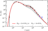 |
Fig. 4 Model grid for 0.1 μm solid, spherical amC dust grains in a present-day wind and detached shell. The best-fitting model isplotted as the red line; the other models, showing present-day mass-loss rates from 5 × 10⁻¹² to 1 × 10⁻⁹ M⊙ yr−1 and detached-shell masses from 5 × 10⁻⁶ to 7 × 10⁻⁵ M⊙, are shown with grey lines. |
4.2 Changing the dust grain properties
In the following, we explore the parameter space of different dust properties and study how they influence the estimate of the detached-shell dust mass. We explore the effect on the model SED of the assumed optical constants, grain composition, grain size, and geometrical grain model.
4.2.1 Optical constants
The basis of dust radiative transfer modelling lies in the description of the radiative dust grain properties, which are defined by optical constants (n and k) that are used to derive the frequency-dependent absorption and scattering opacities. However, since the optical constants are measured in laboratory experiments by different researchers under different conditions, the choice of optical constants can influence the modelling results – even for theoretically identical dust particles. We show this effect by plotting the best-fitting model for 0.1 μm sized solid amC grains in the present-day wind and detached shell using the results from Sect. 4.1 for different sets of opacities (Fig. 5), derived by Preibisch et al. (1993); Rouleau & Martin (1991); Suh (2000); Zubko et al. (1996); and Jager et al. (1998). The greatest change between the different opacities can be seen in the infrared region of the SED at λ > 20μm. The opacities might therefore influence the best-fitting shell mass.
We ran a grid of models varying the present-day mass-loss rate and shell mass for each of the optical constants shown in Fig. 5. The best-fitting models for the different optical constant were then compared to the one when using optical constants by Suh (2000). The best-fitting mass-loss parameters for all tested opacities are presented in Table 2. The  of the opacities by Suh (2000); Preibisch et al. (1993); and Zubko et al. (1996) are equally good, while the derived shell masses for these three opacities are slightly different.
The model grids for the Zubko et al. (1996) and Preibisch et al. (1993) opacities are presented in Fig. A.1. For the Zubko et al. (1996) opacities, a best-fitting present-day wind mass-loss rate of 1 × 10⁻¹⁰ M⊙ yr−1 and a best-fitting detached-shell mass of (2.1 ± 0.3) × 10−5 M⊙ are found. For the Preibisch et al. (1993) opacities, a best-fitting present-day wind mass-loss rate of 1 × 10⁻¹⁰ M⊙ yr−1 and a best-fitting detached-shell mass of (1.9 ± 0.3) × 10−5 M⊙ are found. In comparison to the best-fitting mass-loss parameters found with Suh (2000) opacities, the present-day mass-loss rate decreased by a factor of two, while the best-fitting shell mass decreased by a factor of about 1.5 for both opacities. The change in shell mass is above the 1σ level of the best-fitting model calculated with Suh (2000) opacities.
For the further investigation (unless otherwise mentioned), we always used the opacities by Suh (2000) and assumed the present-day wind to consist of 0.1 μm sized grains with a mass-loss rate of 2 × 10⁻¹⁰ M⊙ yr−1. The Suh (2000) opacities are the most recent measurements, and allow for a direct comparison to previous models by Schöier et al. (2005).
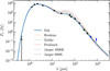 |
Fig. 5 Effectof the different opacities on the SED (detailed model setup described in Sect. 4.2.1). The best-fitting model is drawn with a solid line, while the other models, corresponding to different opacities, are plotted as dotted lines. |
Best-fitting mass-loss parameters for the tested opacities.
4.2.2 Grain composition
All previous models were calculated with the dusty wind consisting of pure amorphous carbon, which is a valid first assumption but in general not what is expected in circumstellar environments. Typical dust species that are found in CSEs of carbon-rich AGB star are magnesium sulfide (MgS) and silicon carbide (SiC). For R Scl, we adopted literature abundances of 4% for MgS (Hony & Bouwman 2004, detailed modelling of R Scl) and 10% for SiC (Sacuto et al. 2011, fitting procedure for R Scl), respectively. To test the influence of these two dust species on the modelled SED and derive the best-fitting shell mass, we computed models with the standard parameters (2 × 10⁻¹⁰ M⊙ yr−1 and 3 × 10⁻⁵ M⊙) for a set of models with 4% MgS and 10% SiC and a set of more extreme abundances (20% MgS; 20% SiC) in both the present-day wind and the shell. For these models, the grains are not in thermal contact. In the more extreme case, thermal contact decreases the shell temperature by approximately 10%, but does not change the estimated dust shell mass significantly.
The results are shown in Fig. 6. It is evident that the general influence on the shape of the SED is almost negligible for the realistic abundances. The effect is very weak even for the more extreme abundances. This is expected, since the introductionof these dust species will mainly lead to the introduction of material specific emission features at distinct wavelengths (~30 μm for MgS and ~11 μm for SiC). The MgS feature is slightly visible for the models with high MgS content (right panel of Fig. 6), while the SiC feature is not seen in the modelled SED at all.
In addition to the qualitative analysis of the shape of the SED, we also derived the best-fitting shell masses for all calculated mixtures of dust species. The results are presented in Table 3. As expected, adding a significantly large amount of dust grains with different optical properties will increase the total shell mass needed to reproduce the SED well. This effect is still within the errors of realistic abundances, but for unrealistically high abundances of MgS and SiC, the shell mass increases significantly up to a factor of 1.5 for the case where 20% MgS and SiC and only 60% amC are present. We conclude that the shell mass is not influenced significantly for realistic MgS and SiC abundances.
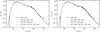 |
Fig. 6 Model grid for a set of different abundances of MgS and SiC. Left: set of abundances based on literature values. Right: set of high abundances. The present-day mass-loss is 2 × 10⁻¹⁰ M⊙ yr−1, and the detached-shell mass is 3 × 10⁻⁵ M⊙. |
Best-fitting mass-loss parameters for the tested mixtures of dust species (amC, MgS, SiC).
4.2.3 Grain sizes
The size of the dust grains will determine the temperature, and hence the black-body emission, of the grains. In particular, large grains at the same distance from the star as small grains will have a lower temperature, contributing more to the long-wavelength part of the shell. We probed the influence of larger dust grains, contributing to a cooler dust component in the SED, on the derived dust shell mass. For the sake of simplicity, we assumed a single grain size (0.1 μm) in the present-day wind and a two-component population of grains in the shell, with 0.1 μm grains and a population of larger grains. The radii of the large grains were 0.25, 0.5, 0.75, 1, 2, and 5 μm. For this analysis, we did not run a whole grid of MCMax models, but assumed optically thin emission to derive scaled models for the mix of large and small grains in the shell (as explained in Sect. 3.8). For each model we varied the mass in the small and large grains to determine the best-fit to the SED. Since we only changed the properties of the dust in the shell, we now only fit the SED to points between 20 μm < λ ≤ 350 μm. The results of this grid of models can be found in Table 4.
From the  values it is obvious that adding large grains to the shell deteriorates the model fit compared to the model with only small grains in the shell. For all large grain sizes except 0.75 μm, the majority of the mass is located in small grains, while only a very small fraction of mass is located in large grains. For 0.75 μm sized grains in the shell, the mass distribution is the opposite, which emphasises the high degeneracy of the models (as described in more detail below). The total mass of the shell increases slightly with increasingly larger grain size. Overall, the
  value decreases slightly with larger grain sizes (for the models including large grains).
Figures 7–9 show the best-fitting SED as well as the corresponding χ2 map for the smallest (0.25 μm), one intermediate (0.75 μm), and for the largest (5 μm) grain sizes we modelled. From the χ2 maps of 0.25 and 0.75 μm large grains, it is obvious that the mass ratio between 0.1 μm and larger grains is highly degenerate, and similarly good results can be achieved with a reverse mass ratio between small and large grains. The larger the large grains, the more the degeneracy dissolves, and for 5 μm sized large grains, the small grains dominate the shell mass, i.e. large grains do not significantly contribute to the total mass in the detached shell. Additionally, the long-wavelength part of the SED where the LABOCA excess emission is visible is not influenced by grains smaller than and equal to 5 μm.
Best-fitting mass-loss parameters for the addition of large grains to the shell.
 |
Fig. 7 Left: best-fitting model SED (purple solid line) consisting of the stellar and present-day wind contribution (grey dotted line), a detached-shell contribution of 0.1 μm grains (purple dashed line), and an additional shell contribution of 0.25 μm grains (magenta dot-dashed line). The wind parameters are 2 × 10⁻¹⁰ M⊙ yr−1 in 0.1 μm sized grains for the present-day wind, 3.00 × 10⁻⁵ M⊙ in the 0.1 μm grain shell, and 1.05 × 10⁻⁶ M⊙ in the 0.25 μm grain shell, derived for solid sphere amC grains. Right: χ-square map for the grid of different shell masses for small (0.1 μm) and large (0.25 μm) sized grains. The grey contour shows the 1σ level on the best-fitting χ-square value. |
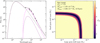 |
Fig. 8 Left: best-fitting model SED (purple solid line) consisting of the stellar and present-day wind contribution (grey dotted line), a detached-shell contribution of 0.1 μm grains (purple dashed line), and an additional shell contribution of 0.75 μm grains (magenta dot-dashed line). The wind parameters are 2 × 10⁻¹⁰ M⊙ yr−1 in 0.1 μm sized grains for the present-day wind, 1.97 × 10⁻⁶ M⊙ in the 0.1 μm grain shell, and 3.00 × 10⁻⁵ M⊙ in the 0.75 μm grain shell, derived for solid sphere amC grains. Right: χ-square map for the grid of different shell masses for small (0.1 μm) and large (0.75 μm) sized grains. The grey contour shows the 1σ level on the best-fitting χ-square value. |
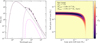 |
Fig. 9 Left: best-fitting model SED (purple solid line) consisting of the stellar and present-day wind contribution (grey dotted line), a detached-shell contribution of 0.1 μm grains (purple dashed line), and an additional shell contribution of 5 μm grains (magenta dot-dashed line). The wind parameters are 2 × 10⁻¹⁰ M⊙ yr−1 in 0.1 μm sized grains for the present-day wind, 3.00 × 10⁻⁵ M⊙ in the 0.1 μm grain shell, and 3.7 × 10⁻⁶ M⊙ in the 5 μm grain shell, derived for solid sphere amC grains. Right: χ-square map for the grid of different shell masses for small (0.1 μm) and large (5 μm) sized grains. The grey contour shows the 1σ level on the best-fitting χ-square value. |
4.2.4 Grain geometry: hollow spheres and fluffy grains
Our standard dust parameters assume spherical and solid dust grains. However, the dust coagulation process in reality likely favours more complex geometries than that (e.g. Mathis & Whiffen 1989). This is taken into account by alternative geometrical descriptions of astrophysical dust. Two widely used descriptions of geometry in dust radiative transfer modelling are the distribution of hollow spheres (DHS) and continuous distribution of ellipsoidals (CDE). The DHS describes spherical dust grains with a specific radius and a varying amount of vacuum included in the grain interior, leading to different masses for each grain of same size. In the CDE approach, the shape of the grains follows a distribution of ellipsoidals with different axis ratios, while the grains are solid. Min et al. (2003) concluded that the general absorption properties of CDE and DHS grain geometries are very similar and on average not really distinguishable from each other in an SED analysis. We therefore only tested the influence of the DHS geometry on the SED with respectto the changing shell mass. In this case, we changed the dust properties in both the present-day wind and inthe shell. The left panel of Fig. 10 shows the results of a model grid for DHS grains with a maximum vacuum volume fraction of 0.7 (Min et al. 2007). The best-fitting present-day mass-loss rate is 7.5 × 10⁻¹¹ M⊙ yr−1 and the best-fitting detached-shell mass is (1.3 ± 0.2) × 10−5 M⊙. As expected, less mass is needed to achieve the same emission from hollow grains that have the same surface area as the solid grains. Compared to the best-fitting model with solid grains, only 40% of the shell mass is needed for the best fit with DHS grains.
Another approach that most likely represents the most accurate description in terms of dynamic grain growth is the introduction of fluffy grains (e.g. Ossenkopf 1993, and references therein). Such fluffy grains are aggregates of individual small particles that stick together and form a larger, mostly irregular structure. A simple approach to mimic such particles is the method of ballistic agglomeration (BA; e.g. Shen et al. 2008). A library of sample aggregates can be found on the web for different aggregate properties and sizes4. The aggregate dust grain optical properties can be exactly computed by the discrete dipole approximation (DDA). Describing grains in this way is computationally very time-consuming, and the calculation of a single aggregate can take up to several days of computation time, even on advanced computing systems. For an overview on the computation of fluffy grains and their opacities, we refer to Min et al. (2016), who studied the characteristics of aggregate dust grains in the context of protoplanetary disks. They concluded that approximating opacities for aggregate grains by simpler approaches works relatively well in their modelling cases when using DHS-shaped grains in combination with effective medium theory and porosity. One of the main effects of using aggregate grains on the opacity is seen in the sub-millimeter wavelength range, where DHS as well as aggregate grains have a flatter slope than solid spheres. While a full study of the effects of fluffy aggregate dust grains in the CSE of AGB stars on the sub-millimeter SED is beyond the scope of this paper, we still present a simple radiative transfer model madefor an example fluffy aggregate grain (see Fig. 11 for more details) to show the effect at sub-millimeter wavelengths. The results of a model grid for this fluffy grain species are shown in the right panel of Fig. 10. We note that by introducing fluffy grains in the detached shell, the overall shell mass required to reproduce the observed SED decreases, since the effective surface area of fluffy grains is much larger than for spherical grains. The best-fitting model for fluffy grains is given by a present-day mass-loss rate of 1 × 10⁻¹⁰ M⊙ yr−1 and a detached-shell mass of (2.3 ± 0.4) × 10−5 M⊙, which is about three quarters of the shell mass obtained when using solid spherical grains.
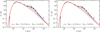 |
Fig. 10 Left: model grid for 0.1 μm sized amC grains described by a DHS model with a maximum volume fraction for vacuum of 0.70; opacities based on Suh (2000). Right: model grid for small, fluffy amC grains (as presented in Fig. 11) with a volume corresponding to the volume of 0.1 μm solid spheres. |
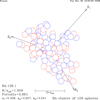 |
Fig. 11 Example fluffy grain model (http://www.astro.princeton.edu/~draine/agglom.html) used for calculating opacities with DDSCAT (Draine & Flatau 1994). This particular grain with an effective size of 0.1 μm is composedof 128 smaller particles. No particle migration is assumed. |
4.3 Sub-millimeter excess
While a variation of the dust properties may change the estimated dust mass in the shell, it does not lead to great changes in the shape of thebest-fitting SED. In particular, none of the models presented here can satisfactorily explain both the emission observed with LABOCA and the data at shorter wavelengths. This excess emission is consistent with emission from the detached shell of dustobserved around R Scl, as shown in Sect. 2.3. Independent observations of R Scl with LABOCA (Program ID: O-079.F-9300A) have a significantly lower signal-to-noise ratio. However, the measured continuum flux is consistent with the measurements given here, hence we judge that the excess emission is real and not due to a calibration error.
It is notstraightforward to find an explanation for the flux observed with LABOCA. Dehaes et al. (2007) detected excess emission at 1.2 mm in a small sub-sample of AGB stars, including R Scl (with a flux of 61.2 mJy at 1.2 mm). They offered a number of possible explanations for the excess flux: (1) contribution from molecular lines, (2) a change in emissivity of the dust grains at the relevant wavelengths, (3) the presence of cold dust, and (4) emission from the photosphere/chromosphere.
We calculated the effects of photometric bandpass correction and molecular line contamination in the LABOCA band and come to the conclusion that both are negligible with respect to the strength of the excess, in line with the conclusions by Dehaes et al. (2007) for regular AGB CSEs. In particular in the case of detached-shell sources, the contribution from molecular lines is likely to be very low because of the photodissociation of molecules in the shell by the interstellar radiation field. In principle, a population of very cold dust grains would add emission at long wavelengths. However, fitting the entire SED for R Scl, including the LABOCA observations, requires adding a black body with a peak at λ ≲ 500 μm. This corresponds to temperatures lower than 5 K (Fig. 12). Not only would this require a population of very large grains, but also for this population to be completely distinct from the population of small grains, since a continuous grain size distribution would lead to a smoother SED shape in the FIR and sub-millimeter, and hence no turn-off to fit both the LABOCA data and the shorter wavelength data. The excess emission is therefore likely not due to thermal emission from dust grains. Finally, the spatial information from the LABOCA and ALMA high-angular observations excludes a photospheric or chromospheric origin of the emission (see Sect. 2.3).
A change in the emission properties from the standard grains generally assumed to be present around AGB stars hence seems to be the most likely explanation for the observed sub-millimeter excess. In the case of R Scl (a carbon AGB star), one possible mechanism may be the presence of polycyclic aromatic hydrocarbons (PAHs; Dehaes et al. 2007). In addition to R Scl and the sources in Dehaes et al. (2007), the same excess is observed in the sub-millimeter in the detached-shell sources U Ant, DR Ser, and V644 Sco (Maercker et al., in prep.), possibly indicating that the grain properties causing the excess may be a general phenomenon in the dust from (carbon) AGB stars.
In observations of the ISM in the Magellanic clouds (Gordon et al. 2014), a similar problem arises where a sub-millimeter excess is detected with Herschel SPIRE that cannot be reproduced by standard dust models. Previous studies by Bot et al. (2010) and Israel et al. (2010) explain the sub-millimeter excess by the introduction of cold dust grains, while a similar excess at longer wavelengths (millimeter to centimeter) is explained by emission due to spinning dust grains. Subsequently, Gordon et al. (2014) tested two scenarios: a change in dust emissivity by introducing a “broken emissivity law” by changing the optical properties of the dust at the relevant wavelengths, and the introduction of a cold temperature dust population. This has a significant effect on the estimated total dust mass in these galaxies; a very cold dust component would potentially contain a hitherto undetected large reservoir of dust mass. However, the authors concluded that a broken emissivity law fits the observations best and that a colder dust component is less likely the origin of the sub-millimeter excess in the Magellanic clouds, in line with the results obtained here. The fact that a very similar excess is observed in the LMC and SMC raises the question of how significant the contribution from AGB stars to the total dust budget is also in low-metallicity galaxies.
We note that without a combination of the SPIRE and LABOCA data, the turn-off in the sub-millimeter would not have been detected. The conclusion without the data at the SPIRE wavelengths would rather have been a continuous grain size population growing to comparatively large grains – a scenario that seems to be excluded now. Observations in the FIR and sub-millimeter are hence essential to properly establish a turn-off in the emissivity in the sub-millimeter, while spatially resolved observations at longer wavelengths (sub-millimeter to millimeter) are needed to constrain the grain properties and determine the origin of the sub-millimeter excess in the detached shell around R Scl and other detached-shell sources.
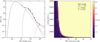 |
Fig. 12 Left: best-fitting model SED (solid line) consisting of the stellar and present-day wind contribution (dotted line), a detached-shell contribution (dashed line), and an additional black body (dot-dashed line). The wind parameters are the best-fitting parameters of 1 × 10⁻¹⁰ M⊙ yr−1 for the present-day wind and 3 × 10⁻⁵ M⊙for the shell mass, derived for 0.1 μm solid sphere amC grains. The best-fitting cool black-body temperature is 5 K. Right: χ-square map for the grid of cool black bodies used to find the best fit. The scaling factor a scales the flux of the black body. |
5 Discussion and conclusions
We modelled the dusty present-day wind and detached shell around R Scl and derived values for the present-day dust mass-loss rate and detached-shell dust mass. We investigated the effect of different dust properties (chemical composition, grain sizes, and geometry) and optical constants on the estimated best-fitting shell mass. We conclude the following:
The observed SED below 350 μm is reproduced equally well, regardless of the dust properties.
-
A change in the implemented optical constants only mildly affects the estimated shell mass.
-
An introduction of realistic amounts of MgS and SiC dust does not have any significant influence on the derived shell mass.
-
Including large grains up to 5 μm in the detached shell does not influence the determined total shell mass and does not improve the fit to the SED.
-
The estimated shell mass is most strongly affected by the geometry of the dust grains. Hollow spheres or fluffy grains require alower dust mass in order to fit the observed SED. Based on this study, the largest uncertainty in determining the return of dust from AGB stars hence lies in the geometrical description of the grains.
-
We observe a significant sub-millimeter excess that cannot be reproduced by any of the models. The origin of this excess is not clear and requires additional observations to determine the spectral index of the dust at sub-millimeter and centimeter wavelengths. A possible explanation is that the opacity of the dust in R Scl (and other carbon stars) has a more complex spectral profile than that considered by us, which could be caused by the presence of PAHs.
We provided a new estimate of the dust mass in the detached shell around R Scl and investigated the dependence of the determined mass on critical grain properties. Based on our models, the upper limit for the shell mass is 3 × 10⁻⁵ M⊙, assuming solid 0.1 μm sized grains. The estimated gas mass in the shell is 4.5 × 10⁻³ M⊙ (Maercker et al. 2016), resulting in a dust-to-gas ratio of 0.007. This value is relatively high compared to results for other carbon-rich AGB stars (Ramstedt et al. 2008). However, if we instead assume DHS grains, the total dust mass decreases by a factor of 2.4 – affecting our estimate of the total dust-masses produced by stars. In that sense, the structure of the dust grains is important when determining the total amount of dust produced from stars and present in galaxies, independent of stellar mass, and when comparing different sources of dust.
In addition to estimating the dust mass in the shell, we also find a significant excess emission in the sub-millimeter. We were unable to constrain the origin of this excess emission. In order to properly constrain the properties of grains around AGB stars, observations at long wavelengths (sub-millimeter to millimeter and possibly centimeter) are also needed.
Acknowledgements
We wish to thank Robin Lombaert for his valuable support and intensive help concerning radiative transfer modelling. M.B. acknowledges funding through the uni:docs fellowship of the University of Vienna. F.K. and M.B. acknowledgefunding by the Austrian Science Fund FWF under project number P23586. M. Maercker acknowledges support from the Swedish Research Council under grant number 2016-03402.
Appendix A Additional opacity models
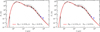 |
Fig. A.1 Model grids calculated with opacities by Zubko et al. (1996) (left) and Preibisch et al. (1993) (right) for 0.1 μm solid, spherical amC dust grains in a present-day wind and detached shell. The best-fitting model is represented with a solid red line, and the respective best-fitting model parameters are given in the legend. The grey lines represent the other models in the grid. |
References
- Bot, C., Ysard, N., Paradis, D., et al. 2010, A&A, 523, A20 [NASA ADS] [CrossRef] [EDP Sciences] [Google Scholar]
- Cox, N. L. J., Kerschbaum, F., van Marle, A.-J., et al. 2012, A&A, 537, A35 [NASA ADS] [CrossRef] [EDP Sciences] [Google Scholar]
- Dehaes, S., Groenewegen, M. A. T., Decin, L., et al. 2007, MNRAS, 377, 931 [NASA ADS] [CrossRef] [Google Scholar]
- Draine, B. T., & Flatau, P. J. 1994, J. Opt. Soc. Am. A, 11, 1491 [NASA ADS] [CrossRef] [Google Scholar]
- Forestini, M., & Charbonnel, C. 1997, A&AS, 123, 241 [NASA ADS] [CrossRef] [EDP Sciences] [Google Scholar]
- González Delgado, D., Olofsson, H., Schwarz, H. E., Eriksson, K., & Gustafsson, B. 2001, A&A, 372, 885 [NASA ADS] [CrossRef] [EDP Sciences] [Google Scholar]
- González Delgado, D., Olofsson, H., Schwarz, H. E., et al. 2003, A&A, 399, 1021 [NASA ADS] [CrossRef] [EDP Sciences] [Google Scholar]
- Gordon, K. D., Roman-Duval, J., Bot, C., et al. 2014, ApJ, 797, 85 [NASA ADS] [CrossRef] [Google Scholar]
- Griffin, M. J., Abergel, A., Abreu, A., et al. 2010, A&A, 518, L3 [Google Scholar]
- Groenewegen, M. A. T., Waelkens, C., Barlow, M. J., et al. 2011, A&A, 526, A162 [NASA ADS] [CrossRef] [EDP Sciences] [Google Scholar]
- Habing, H. J. 1996, A&ARv, 7, 97 [NASA ADS] [CrossRef] [Google Scholar]
- Herwig, F., & Austin, S. M. 2004, ApJ, 613, L73 [NASA ADS] [CrossRef] [Google Scholar]
- Hony, S., & Bouwman, J. 2004, A&A, 413, 981 [NASA ADS] [CrossRef] [EDP Sciences] [Google Scholar]
- Israel, F. P., Wall, W. F., Raban, D., et al. 2010, A&A, 519, A67 [NASA ADS] [CrossRef] [EDP Sciences] [Google Scholar]
- Jager, C., Mutschke, H., & Henning, T. 1998, A&A, 332, 291 [NASA ADS] [Google Scholar]
- Kerschbaum, F., & Hron, J. 1994, A&AS, 106, 397 [NASA ADS] [Google Scholar]
- Knapp, G. R., Pourbaix, D., Platais, I., & Jorissen, A. 2003, A&A, 403, 993 [NASA ADS] [CrossRef] [EDP Sciences] [Google Scholar]
- Kovács, A. 2008, in Millimeter and Submillimeter Detectors and Instrumentation for Astronomy IV, Proc. SPIE, 7020, 70201S [Google Scholar]
- Maercker, M., Mohamed, S., Vlemmings, W. H. T., et al. 2012, Nature, 490, 232 [NASA ADS] [CrossRef] [PubMed] [Google Scholar]
- Maercker, M., Ramstedt, S., Leal-Ferreira, M. L., Olofsson, G., & Floren, H. G. 2014, A&A, 570, A101 [NASA ADS] [CrossRef] [EDP Sciences] [Google Scholar]
- Maercker, M., Vlemmings, W. H. T., Brunner, M., et al. 2016, A&A, 586, A5 [NASA ADS] [CrossRef] [EDP Sciences] [Google Scholar]
- Maercker, M., Brunner, M., Mecina, M., & De Beck, E. 2018, A&A, 611, A102 [Google Scholar]
- Mancini, M., Schneider, R., Graziani, L., et al. 2015, MNRAS, 451, L70 [CrossRef] [Google Scholar]
- Mathis, J. S., & Whiffen, G. 1989, ApJ, 341, 808 [NASA ADS] [CrossRef] [Google Scholar]
- Mattsson, L., Höfner, S., Wahlin, R., & Herwig, F. 2007, in Why Galaxies Care About AGB Stars: Their Importance as Actors and Probes, eds. F. Kerschbaum, C. Charbonnel, & R. F. Wing, ASP Conf. Ser., 378, 239 [Google Scholar]
- Min, M., Hovenier, J. W., & de Koter A. 2003, A&A, 404, 35 [NASA ADS] [CrossRef] [EDP Sciences] [Google Scholar]
- Min, M., Waters, L. B. F. M., de Koter, A., et al. 2007, A&A, 462, 667 [NASA ADS] [CrossRef] [EDP Sciences] [Google Scholar]
- Min, M., Dullemond, C. P., Dominik, C., de Koter, A., & Hovenier, J. W. 2009, A&A, 497, 155 [NASA ADS] [CrossRef] [EDP Sciences] [Google Scholar]
- Min, M., Rab, C., Woitke, P., Dominik, C., & Ménard, F. 2016, A&A, 585, A13 [NASA ADS] [CrossRef] [EDP Sciences] [Google Scholar]
- Olofsson, H., Eriksson, K., & Gustafsson, B. 1988, A&A, 196, L1 [NASA ADS] [Google Scholar]
- Olofsson, H., Carlstrom, U., Eriksson, K., Gustafsson, B., & Willson, L. A. 1990, A&A, 230, L13 [NASA ADS] [Google Scholar]
- Olofsson, H., Bergman, P., Eriksson, K., & Gustafsson, B. 1996, A&A, 311, 587 [NASA ADS] [Google Scholar]
- Olofsson, H., Maercker, M., Eriksson, K., Gustafsson, B., & Schöier, F. 2010, A&A, 515, A27 [NASA ADS] [CrossRef] [EDP Sciences] [Google Scholar]
- Ossenkopf, V. 1993, A&A, 280, 617 [NASA ADS] [Google Scholar]
- Poglitsch, A., Waelkens, C., Geis, N., et al. 2010, A&A, 518, L2 [NASA ADS] [CrossRef] [EDP Sciences] [Google Scholar]
- Preibisch, T., Ossenkopf, V., Yorke, H. W., & Henning, T. 1993, A&A, 279, 577 [NASA ADS] [Google Scholar]
- Ramstedt, S., Schöier, F. L., Olofsson, H., & Lundgren, A. A. 2008, A&A, 487, 645 [NASA ADS] [CrossRef] [EDP Sciences] [Google Scholar]
- Rouleau, F., & Martin, P. G. 1991, ApJ, 377, 526 [NASA ADS] [CrossRef] [Google Scholar]
- Sacuto, S., Aringer, B., Hron, J., et al. 2011, A&A, 525, A42 [NASA ADS] [CrossRef] [EDP Sciences] [Google Scholar]
- Schneider, R., Valiante, R., Ventura, P., et al. 2014, MNRAS, 442, 1440 [NASA ADS] [CrossRef] [Google Scholar]
- Schöier, F. L., Lindqvist, M., & Olofsson, H. 2005, A&A, 436, 633 [NASA ADS] [CrossRef] [EDP Sciences] [Google Scholar]
- Shen, Y., Draine, B. T., & Johnson, E. T. 2008, ApJ, 689, 260 [NASA ADS] [CrossRef] [Google Scholar]
- Siringo, G., Kreysa, E., Kovács, A., et al. 2009, A&A, 497, 945 [NASA ADS] [CrossRef] [EDP Sciences] [Google Scholar]
- Steffen, M., & Schönberner, D. 2000, A&A, 357, 180 [NASA ADS] [Google Scholar]
- Suh, K.-W. 2000, MNRAS, 315, 740 [NASA ADS] [CrossRef] [Google Scholar]
- Wittkowski, M., Hofmann, K.-H., Höfner, S., et al. 2017, A&A, 601, A3 [NASA ADS] [CrossRef] [EDP Sciences] [Google Scholar]
- Zubko, V. G., Mennella, V., Colangeli, L., & Bussoletti, E. 1996, MNRAS, 282, 1321 [NASA ADS] [CrossRef] [Google Scholar]
This publication is based on data acquired with the Atacama Pathfinder Experiment (APEX). APEX is a collaboration between the Max-Planck-Institut für Radioastronomie, the European Southern Observatory, and the Onsala Space Observatory.
All Tables
Best-fitting mass-loss parameters for the tested mixtures of dust species (amC, MgS, SiC).
All Figures
|
Fig. 1 SED of R Scl. Black: points used in Schöier et al. (2005); green: Herschel/PACS; blue: Herschel/SPIRE; red: LABOCA; purple: ALMA. Plotted with the grey dashed line is the overall best-fit model of the star, present-day wind, and detached shell (see Sect. 4.1). |
| In the text | |
|
Fig. 2 Top: LABOCA observations towards R Scl. The colour scale is given in Jy beam−1. Middle: LABOCA map with the stellar SED (retrieved from the ALMA continuum observations convolved by the LABOCA beam) subtracted. Bottom: residual map after subtracting the stellar SED and a spherical detached shell with a radius of 18′′.5 and width of 2′′. The structures in the residual map are due to asymmetric emission from the shell, consistent with scattered-light observations. |
| In the text | |
|
Fig. 3 Model grid of black bodies with different luminosities and effective temperatures (grey lines). The best-fitting model is shown as a red line. All SED data points below 4 μm are used for χ-square fitting (black dots); data points with wavelengths longer than that are plotted in grey; the ALMA data points are shown in blue for reference. |
| In the text | |
|
Fig. 4 Model grid for 0.1 μm solid, spherical amC dust grains in a present-day wind and detached shell. The best-fitting model isplotted as the red line; the other models, showing present-day mass-loss rates from 5 × 10⁻¹² to 1 × 10⁻⁹ M⊙ yr−1 and detached-shell masses from 5 × 10⁻⁶ to 7 × 10⁻⁵ M⊙, are shown with grey lines. |
| In the text | |
|
Fig. 5 Effectof the different opacities on the SED (detailed model setup described in Sect. 4.2.1). The best-fitting model is drawn with a solid line, while the other models, corresponding to different opacities, are plotted as dotted lines. |
| In the text | |
|
Fig. 6 Model grid for a set of different abundances of MgS and SiC. Left: set of abundances based on literature values. Right: set of high abundances. The present-day mass-loss is 2 × 10⁻¹⁰ M⊙ yr−1, and the detached-shell mass is 3 × 10⁻⁵ M⊙. |
| In the text | |
|
Fig. 7 Left: best-fitting model SED (purple solid line) consisting of the stellar and present-day wind contribution (grey dotted line), a detached-shell contribution of 0.1 μm grains (purple dashed line), and an additional shell contribution of 0.25 μm grains (magenta dot-dashed line). The wind parameters are 2 × 10⁻¹⁰ M⊙ yr−1 in 0.1 μm sized grains for the present-day wind, 3.00 × 10⁻⁵ M⊙ in the 0.1 μm grain shell, and 1.05 × 10⁻⁶ M⊙ in the 0.25 μm grain shell, derived for solid sphere amC grains. Right: χ-square map for the grid of different shell masses for small (0.1 μm) and large (0.25 μm) sized grains. The grey contour shows the 1σ level on the best-fitting χ-square value. |
| In the text | |
|
Fig. 8 Left: best-fitting model SED (purple solid line) consisting of the stellar and present-day wind contribution (grey dotted line), a detached-shell contribution of 0.1 μm grains (purple dashed line), and an additional shell contribution of 0.75 μm grains (magenta dot-dashed line). The wind parameters are 2 × 10⁻¹⁰ M⊙ yr−1 in 0.1 μm sized grains for the present-day wind, 1.97 × 10⁻⁶ M⊙ in the 0.1 μm grain shell, and 3.00 × 10⁻⁵ M⊙ in the 0.75 μm grain shell, derived for solid sphere amC grains. Right: χ-square map for the grid of different shell masses for small (0.1 μm) and large (0.75 μm) sized grains. The grey contour shows the 1σ level on the best-fitting χ-square value. |
| In the text | |
|
Fig. 9 Left: best-fitting model SED (purple solid line) consisting of the stellar and present-day wind contribution (grey dotted line), a detached-shell contribution of 0.1 μm grains (purple dashed line), and an additional shell contribution of 5 μm grains (magenta dot-dashed line). The wind parameters are 2 × 10⁻¹⁰ M⊙ yr−1 in 0.1 μm sized grains for the present-day wind, 3.00 × 10⁻⁵ M⊙ in the 0.1 μm grain shell, and 3.7 × 10⁻⁶ M⊙ in the 5 μm grain shell, derived for solid sphere amC grains. Right: χ-square map for the grid of different shell masses for small (0.1 μm) and large (5 μm) sized grains. The grey contour shows the 1σ level on the best-fitting χ-square value. |
| In the text | |
|
Fig. 10 Left: model grid for 0.1 μm sized amC grains described by a DHS model with a maximum volume fraction for vacuum of 0.70; opacities based on Suh (2000). Right: model grid for small, fluffy amC grains (as presented in Fig. 11) with a volume corresponding to the volume of 0.1 μm solid spheres. |
| In the text | |
|
Fig. 11 Example fluffy grain model (http://www.astro.princeton.edu/~draine/agglom.html) used for calculating opacities with DDSCAT (Draine & Flatau 1994). This particular grain with an effective size of 0.1 μm is composedof 128 smaller particles. No particle migration is assumed. |
| In the text | |
|
Fig. 12 Left: best-fitting model SED (solid line) consisting of the stellar and present-day wind contribution (dotted line), a detached-shell contribution (dashed line), and an additional black body (dot-dashed line). The wind parameters are the best-fitting parameters of 1 × 10⁻¹⁰ M⊙ yr−1 for the present-day wind and 3 × 10⁻⁵ M⊙for the shell mass, derived for 0.1 μm solid sphere amC grains. The best-fitting cool black-body temperature is 5 K. Right: χ-square map for the grid of cool black bodies used to find the best fit. The scaling factor a scales the flux of the black body. |
| In the text | |
|
Fig. A.1 Model grids calculated with opacities by Zubko et al. (1996) (left) and Preibisch et al. (1993) (right) for 0.1 μm solid, spherical amC dust grains in a present-day wind and detached shell. The best-fitting model is represented with a solid red line, and the respective best-fitting model parameters are given in the legend. The grey lines represent the other models in the grid. |
| In the text | |
Current usage metrics show cumulative count of Article Views (full-text article views including HTML views, PDF and ePub downloads, according to the available data) and Abstracts Views on Vision4Press platform.
Data correspond to usage on the plateform after 2015. The current usage metrics is available 48-96 hours after online publication and is updated daily on week days.
Initial download of the metrics may take a while.