| Issue |
A&A
Volume 614, June 2018
|
|
|---|---|---|
| Article Number | A89 | |
| Number of page(s) | 4 | |
| Section | The Sun | |
| DOI | https://doi.org/10.1051/0004-6361/201731887 | |
| Published online | 20 June 2018 | |
Spatial variations of the Sr I 4607 Å scattering polarization peak
1
Istituto Ricerche Solari Locarno, IRSOL, associated to Università della Svizzera italiana,
Locarno, Switzerland
e-mail: This email address is being protected from spambots. You need JavaScript enabled to view it.
2
Kiepenheuer Institut für Sonnenforschung,
Freiburg, Germany
3
ETHZ,
Zurich, Switzerland
Received:
29
December
2017
Accepted:
13
February
2018
Abstract
Context. The scattering polarization signal observed in the photospheric Sr I 4607 Å line is expected to vary at granular spatial scales. This variation can be due to changes in the magnetic field intensity and orientation (Hanle effect), but also to spatial and temporal variations in the plasma properties. Measuring the spatial variation of such polarization signal would allow us to study the properties of the magnetic fields at subgranular scales, but observations are challenging since both high spatial resolution and high spectropolarimetric sensitivity are required.
Aims. We aim to provide observational evidence of the polarization peak spatial variations, and to analyze the correlation they might have with granulation.
Methods. Observations conjugating high spatial resolution and high spectropolarimetric precision were performed with the Zurich IMaging POLarimeter, ZIMPOL, at the GREGOR solar telescope, taking advantage of the adaptive optics system and the newly installed image derotator.
Results. Spatial variations of the scattering polarization in the Sr I 4607 Å line are clearly observed. The spatial scale of these variations is comparable with the granular size. Small correlations between the polarization signal amplitude and the continuum intensity indicate that the polarization is higher at the center of granules than in the intergranular lanes.
Key words: Sun: photosphere / Sun: granulation / polarization / scattering / instrumentation: high angular resolution / magnetic fields
© ESO 2018
1 Introduction
The Sr I 4607 Å line shows one of the strongest scattering polarization signals in the visible solar spectrum; this line was observed for the first time at Istituto Ricerche Solari Locarno, IRSOL, by Wiehr (1975). On the basis of 3D simulations, Trujillo Bueno & Shchukina (2007) predicted spatial variations in the amplitude of this signal, provided that the granulation were resolved. These fluctuations originate from local variations in the anisotropy of the radiation field, as well as from variations in the magnetic field between granule interiors and intergranular lanes. Several attempts to observe this behavior have been made, and a first indication of differential depolarization in granular interiors and intergranular lanes was found by Malherbe et al. (2007). Using the Zurich IMaging POLarimeter, ZIMPOL, (Ramelli et al. 2010) at the Gregory Coudé telescope at IRSOL (45 cm aperture), we were only able to measure sporadic spatial variations of the linear polarization peak of the Sr I 4607 Å line, at scales well above the granular one. Other observations are currently performed with the same aim by a group at the Max Planck Institute for Solar System Research; this group has obtained positive results (Zeuner & Feller, priv. comm.).
We report here the results of the observing campaign we performed in 2016 at the GREGOR solar telescope in Tenerife (Schmidt et al. 2012), using the ZIMPOL polarimeter (Ramelli et al. 2014). The seeing conditions during the campaign allowed us to achieve the required spatial resolution during only a few hours, when we chose to observe a quiet region near the East limb. We could reach a subarcsecond spatial resolution (we estimate about 0.6′′), which allowed us to detect the expected fluctuations in the linear polarization.
Hereafter we define as positive Stokes Q the linear polarization parallel to the closest solar limb. In addition to spatial variations in the amplitude of the Q∕I scattering polarization signal, we also detected weak U∕I signals, with amplitudes just above the instrumental noise level.
In the next sections we describe the observations and the reduction, and we investigate the possible presence of correlations between the spatial variations of the polarization signals and those of the continuum intensity, which we have used as an indicator of the location of granules and intergranular lanes.
2 Observations
Observations were performed on October 12, 2016, at the GREGOR telescope in Tenerife, using the ZIMPOL polarimeter (see Ramelli et al. 2014, for technical details), which is installed on the same spectrograph that is used for the GREGOR Infrared Spectrograph, GRIS, (Collados et al. 2012). The double ferroelectric crystal (FLC) modulator (Gisler et al. 2003) was installed at the entrance of the spectrograph. The 1 kHz modulation allowed us to simultaneously measure the full Stokes vector without significant influences from the seeing; the polarimetric precision is thus principally determined by the photon noise. For the observations we took advantage of the recently installed image derotator, which allowed us to perform long-exposure observations. The observations were performed close to the east limb, at μ = cos θ ≃ 0.3 (where θ is the heliocentric angle). The solar surface was thus observed under an angle of ≃70 deg.
Small pores were present in the field of view and could be used by the Shack Hartmann wavefront sensor of the adaptive optics system (Berkefeld et al. 2016). The spectrograph slit was placed away from the pores, in a magnetically quiet region, parallel to the closest limb. The seeing quality varied during the observation. The Fried parameter oscillated between r0 = 10 cm and r0 = 20 cm. The solar area covered by the spectrograph slit corresponded to 0.3′′ (width of the slit) times 47′′ (length portion of the slit covered by the CCD sensor). Along the spatial direction, a ZIMPOL image has 140 pixels, so that one pixel row covered 0.33′′. Taking into account stray light in the telescope, residual effects that could not be fully corrected by the adaptive optics, and the sampling theorem, we estimate to have achieved a spatial resolution of about 0.6′′.
The GREGOR polarimetric calibration unit, GPU, (Hofmann et al. 2012) was used. This device is located at the second focal point (F2) before any folding reflection that would produce significant instrumental polarization.
Four single acquisitions with 1 s exposure time each are needed to collect the required minimum information to calculate a Stokes image with reduced systematic instrumental noise (Gisler 2005). Each Stokes image thus required 6.7 s (total exposure time plus the time required for digitization and data transfer).
The complete observing procedure in a selected solar region consisted of the following steps:
-
Calculation of the ZIMPOL camera timing parameters needed to reduce systematic effects that might be introduced by large instrumental polarization. To this aim, the specific procedure described in Ramelli et al. (2014) was applied. Measurements were made in quiet-Sun regions.
-
The polarimetric calibration was performed using the GPU located at F2; data were collected and used to determine the demodulation matrix. In addition, a dark current image was stored.
-
A flatfield observation was taken by moving the telescope in an area away from the solar limb and avoiding active regions as much as possible.
-
The scientific observation of the selected region was performed.
In orderto follow the evolution of the demodulation matrix and of the intensity flatfield image with the rotation of the telescope, all these operations typically had to be repeated every 20 to 40 min. A total of five series of observations were performed at μ ≃ 0.3, but with the slitlocated at slightly different positions. The number of images stored in each series was 25, 250, 125, 125, and 125.
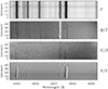 |
Fig. 1 Stokes images of a spectral interval around the Sr I 4607 Å line. The spatial direction spans 47′′ on the solar disk. The observed region was near the est limb at μ ≃ 0.3, and the slit was placed parallel to the nearest limb. The reference direction for positive Stokes Q is the tangent to the nearest solar limb. These images are the result of a 2-minute observation average. The granulation pattern can be recognized in the intensity image, in particular in the continuum. The Q∕I image showsthe scattering polarization peak in the core of the Sr I line. Spatial variations at granular scales of this peak can be observed. Weak U∕I signals, just above the noise level, can be observed in the core of the Sr I line. In V∕I the typical antisymmetric Zeeman patterns can be easily recognized. Note in particular some small sized V∕I structures (for instance at spatial position 27′′). |
3 Data reduction
The Stokes images acquired with the ZIMPOL camera were corrected through the calibration matrix, which was calculated from the data collected during the polarization calibration procedure. The intensity images were corrected for flatfield.
The root mean square (rms) obtained in an area located in the continuum in the fractional polarization images (obtained in 6.7 s) is equal to ≃0.0028, and it is mainly given by the statistical noise. This value is comparable to the amplitude of the signals we are interested in measuring. We therefore needed to average various images to improve the signal-to-noise ratio to preserve the spatial and spectral resolutions.
Figure 1 shows the images obtained by averaging 20 Stokes images that were sequentially registered. In the I image we can recognize intensity variations along the spatial direction due to the granulation. The Q∕I image shows the scattering polarization peak in the Sr I 4607 Å line. The polarization peak shows clear spatial variations; detection these was in fact the main goal of our observations. In the U∕I image it is possible to note weak signals in the Sr I line core. Finally, in the V∕I image, we can recognize the typical patterns of the longitudinal Zeeman effect. This image allows appreciating the high spatial resolution (≃ 0.6′′) of our observation.
Averaging 20 subsequent Stokes images, which corresponds to an integration over about two minutes, we were able to reach a polarimetric sensitivity of ≃7.5 × 10⁻⁴. A discussion of the suitability of this temporal average is provided in the next section. The spectral resolution of our observation is of ≃10 mÅ.
4 Data analysis and results
We here focus our attention on the second series of observations that consists of 250 images, because this series has more data. Our goal is to analyze the spatial variations in the linear polarization in the Sr I 4607 Å line, and to obtain some insights on the physical information that can be extracted from them. In a first attempt we try to correlate the amplitude of the Q∕I peak with the continuum intensity.
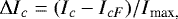
As previously pointed out, in order to obtain an adequate signal-to-noise ratio in the polarization images, we averaged 20 subsequent images of the time series, corresponding to an integration over about two minutes. To evaluate whether this temporal averaging introduced significant spatial degradation in our data, we visualized the temporal evolution of the intensity seen by the spectrograph slit (the portion seen by the CCD sensor). This is shown in the left panel of Fig. 2, where the continuum intensity is reported in gray scale as a function of the spatial position along the slit (abscissa) and of the time (ordinate). A single continuum intensity profile can be seen as an example in the right panel of the same figure (solid line). The overplotted dotted line is the Fourier-filtered profile that reproduces the large-scale fluctuations, but “cuts” small-scale fluctuations.
Figure 2 shows that the observed structures do not change drastically within several minutes (as might be expected considering the average lifetime of the granules), thus confirming that an average over 20 images is suitable for our investigation. Intensity and polarimetric data were now calculated from images obtained by averaging the time series of 250Stokes images with a smoothing window width of 20 images, shifted in increments of 20 images (to avoid data overlap). Discarding the last 10 images of the time series, we then obtain a sequence of 12 averaged images.
The amplitude (as well as the width and the position) of each Q∕I peak in theSr I was calculated using a Gauss fit. Some examples of single Q∕I peak profiles are provided in Fig. 3, showing measured profiles (solid lines) with different amplitudes, and the corresponding Gaussian fit (dashed line). An estimate of the errors for each fit was also calculated and stored by the fitting procedure. We verified that the averaged amplitude of the Q∕I peaks is compatible with the values reported by Stenflo et al. (1997).
The question arises whether these variations have a solar origin. A solar origin is supported by the following arguments. All the known instrumental sources of spurious signals (that might be introduced by an imprecise optical setup) were carefully investigated and excluded. Moreover, the observed variations are generally larger than the noise affecting each profile (note that the profiles in Fig. 3 are not smoothed). Finally, we verified that these variations disappeared when the spatial resolution was lower (e.g., with bad seeing conditions).
The continuum intensity indicates whether we observe a granulum or an intergranulum. We introduce the following parameter:
where Ic is the continuum intensity (e.g., see the solid line in the right panel of Fig. 2), IcF is obtained with Fourier smoothing of Ic (dotted line in the right panel of Fig. 2) that follows the large-scale fluctuation, and Imax is the maximum value in the continuum. The parameter ΔIc provides an approximate indication on whether we observe a granulum (positive sign) or an intergranular lane (negative sign).
The scatter plot in Fig. 4 shows how the Q∕I peak values correlate with the ΔIc parameter. The error in the Q∕I peak amplitudes is estimated by the Gauss fit procedure applied to the profile (± 0.0004). The error bar is reported in the lower left part of Fig. 4.
The points in the scatter plot spread over a region that is larger than the error interval. A linear regression (see solid line) suggests a trend of increasing linear polarization in the granules compared to the intergranules. The slope of the solid line is (4.44 ± 0.5) × 10−4. The Pearson correlation coefficient is 0.19. The trend is an increase in Q∕I peak amplitude toward the interior of the granulation cells. This result was also found by Malherbe et al. (2007).
The U∕I panel in Fig. 1 shows weak signals in the core of the Sr I line. Although their amplitudes are very small, they are expected to be of solar origin. These signals can be either due to the rotation of the scattering polarization plane produced by the Hanle effect caused by weak resolved magnetic fields or to anisotropy variations in the radiation field that are due to horizontal inhomogeneities in the photospheric plasma. If the Zeeman effect were to play a role, we would expect larger signatures in the neighboring Fe I line, which are not observed. The signal-to-noise ratio in U∕I does not allow significant correlation studies between U∕I and other quantities, such as Q∕I or the continuum intensity.
The precision and resolution we were able to achieve in the observations allowed us to perceive a small correlation between thescattering polarization amplitude and the continuum intensity. Observations at different solar positions to observe the atmosphere under different angles would improve the information we can acquire from this technique. With current observing facilities, even with ideal observing conditions, it is not expected to achieve results with a much better significance. The main limit is imposed by the noise given by the available photon statistics. Significant improvements are expected with the future 4-meter class telescopes such as the Daniel K. Inouye Solar Telescope, DKIST, andthe European Solar Telescope, EST.
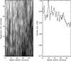 |
Fig. 2 Left panel: 2D image composed by the 250 continuum intensity profiles measured along the spatial direction (47′′) and sequentially plotted along the ordinate. The time required to store a Stokes image is 6.7 s. The 250 profiles thus report the evolution of the intensity seen by the spectrograph slit in 28 min. Right panel: one of the 250 continuum intensity profiles (solid line). The dotted line is a smoothed profile obtained by applying a Fourier filter to remove fluctuations at granular scale. |
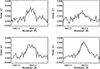 |
Fig. 3 Q∕I profiles in awavelength interval around the Sr I line. The profiles correspond to a single row of pixels in the spatial direction. The dashed lines are Gaussian fits of the profiles, and are used to calculate the polarization peak amplitude. |
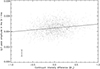 |
Fig. 4 Scatter plot of the Sr I Q∕I peak amplitude vs. the corrected continuum intensity (see text). The error bar associated with each Q∕I value is shown in the bottom left corner. The solid line is a linear regression indicating a trend with a Pearson correlation coefficient of 0.19. |
5 Conclusions
Our observations allowed the detection of spatial variations of the Q∕I scattering polarization signal of the Sr I 4607 Å line, measured at μ ≃ 0.3 (the direction of positive Stokes Q is parallel to the nearest solar limb). The spatial scale of the variations is comparable to the granular scale, thus their origin has to be searched for in physical effects that occur at this level. We also detected small spatial scale U∕I signatures, but with polarimetric amplitudes that are just above the noise level and cannot be easily analyzed.
These small-scale signatures might be produced by the Hanle effect (depolarization and the rotation of the scattering polarization plane due to oriented magnetic fields) by geometrical or dynamic anisotropy fluctuations of the radiation field.
We find a small correlation between the scattering polarization peak amplitudes of the Sr I 4607 Å line and the continuum intensity. This suggests that the polarization inside granulation cells is higher than in the lanes.
The significance of the results presented here is mainly limited by the available photon statistics. Significant improvements in this sense are expected from the next generation of solar telescopes such as the DKIST and the EST.
Acknowledgements
The 1.5 meter GREGOR solar telescope was built by a German consortium under the leadership of the Kiepenheuer-Institut für Sonnenphysik in Freiburg with the Leibniz-Institut für Astrophysik Potsdam, the Institut für Astrophysik Göttingen, and the Max-Planck-Institut für Sonnensystemforschung in Göttingen as partners, and with contributions by the Instituto de Astrofsica de Canarias and the Astronomical Institute of the Academy of Sciences of the Czech Republic. IRSOL is supported by the Swiss Confederation (SEFRI), Canton Ticino, the city of Locarno and the local municipalities. This research work was financed by SNF grants 200020_157103 and 200020_169418.
References
- Berkefeld, T., Schmidt, D., Soltau, D., Heidecke, F., & Fischer, A. 2016, in Adaptive Optics Systems V, Proc. SPIE, 9909, 990924 [CrossRef] [Google Scholar]
- Collados, M., López, R., Páez, E., et al. 2012, Astron. Nachr., 333, 872 [NASA ADS] [CrossRef] [Google Scholar]
- Gisler, D. 2005, Phd thesis, ETH-Zurich, Switzerland [Google Scholar]
- Gisler, D., Feller, A., & Gandorfer, A. M. 2003, in Polarimetry in Astronomy, ed. S. Fineschi, Proc. SPIE, 4843, 45 [NASA ADS] [CrossRef] [Google Scholar]
- Hofmann, A., Arlt, K., Balthasar, H., et al. 2012, Astron. Nachr., 333, 854 [NASA ADS] [CrossRef] [Google Scholar]
- Malherbe, J.-M., Moity, J., Arnaud, J., & Roudier, T. 2007, A&A, 462, 753 [NASA ADS] [CrossRef] [EDP Sciences] [Google Scholar]
- Ramelli, R., Balemi, S., Bianda, M., et al. 2010, in SPIE Conf. Ser., 7735 [Google Scholar]
- Ramelli, R., Gisler, D., Bianda, M., et al. 2014, in Ground-based and Airborne Instrumentation for Astronomy V, SPIE Conf. Ser., 9147, 91473G [Google Scholar]
- Schmidt, W., von der Lühe, O., Volkmer, R., et al. 2012, Astron. Nachr., 333, 796 [NASA ADS] [CrossRef] [Google Scholar]
- Stenflo, J. O., Bianda, M., Keller, C. U., & Solanki, S. K. 1997, A&A, 322, 985 [NASA ADS] [Google Scholar]
- Trujillo Bueno, J., & Shchukina, N. 2007, ApJ, 664, L135 [NASA ADS] [CrossRef] [Google Scholar]
- Wiehr, E. 1975, A&A, 38, 303 [NASA ADS] [Google Scholar]
All Figures
|
Fig. 1 Stokes images of a spectral interval around the Sr I 4607 Å line. The spatial direction spans 47′′ on the solar disk. The observed region was near the est limb at μ ≃ 0.3, and the slit was placed parallel to the nearest limb. The reference direction for positive Stokes Q is the tangent to the nearest solar limb. These images are the result of a 2-minute observation average. The granulation pattern can be recognized in the intensity image, in particular in the continuum. The Q∕I image showsthe scattering polarization peak in the core of the Sr I line. Spatial variations at granular scales of this peak can be observed. Weak U∕I signals, just above the noise level, can be observed in the core of the Sr I line. In V∕I the typical antisymmetric Zeeman patterns can be easily recognized. Note in particular some small sized V∕I structures (for instance at spatial position 27′′). |
| In the text | |
|
Fig. 2 Left panel: 2D image composed by the 250 continuum intensity profiles measured along the spatial direction (47′′) and sequentially plotted along the ordinate. The time required to store a Stokes image is 6.7 s. The 250 profiles thus report the evolution of the intensity seen by the spectrograph slit in 28 min. Right panel: one of the 250 continuum intensity profiles (solid line). The dotted line is a smoothed profile obtained by applying a Fourier filter to remove fluctuations at granular scale. |
| In the text | |
|
Fig. 3 Q∕I profiles in awavelength interval around the Sr I line. The profiles correspond to a single row of pixels in the spatial direction. The dashed lines are Gaussian fits of the profiles, and are used to calculate the polarization peak amplitude. |
| In the text | |
|
Fig. 4 Scatter plot of the Sr I Q∕I peak amplitude vs. the corrected continuum intensity (see text). The error bar associated with each Q∕I value is shown in the bottom left corner. The solid line is a linear regression indicating a trend with a Pearson correlation coefficient of 0.19. |
| In the text | |
Current usage metrics show cumulative count of Article Views (full-text article views including HTML views, PDF and ePub downloads, according to the available data) and Abstracts Views on Vision4Press platform.
Data correspond to usage on the plateform after 2015. The current usage metrics is available 48-96 hours after online publication and is updated daily on week days.
Initial download of the metrics may take a while.