| Issue |
A&A
Volume 614, June 2018
|
|
|---|---|---|
| Article Number | A50 | |
| Number of page(s) | 6 | |
| Section | Cosmology (including clusters of galaxies) | |
| DOI | https://doi.org/10.1051/0004-6361/201731160 | |
| Published online | 12 June 2018 | |
Lensing of fast radio bursts by binaries to probe compact dark matter
1
School of Astronomy and Space Science, Nanjing University,
Nanjing
210093,
PR China
e-mail: fayinwang@nju.edu.cn
2
Key Laboratory of Modern Astronomy and Astrophysics, Nanjing University, Ministry of Education,
Nanjing
210093,
PR China
Received:
12
May
2017
Accepted:
20
January
2018
The possibility that a fraction of dark matter is comprised of massive compact halo objects (MACHOs) remains unclear, especially in the 20–100 M⊙ window. MACHOs could make up binaries, whose mergers may be detected by LIGO as gravitational wave events. On the other hand, the cosmological origin of fast radio burst (FRBs) has been confirmed. We investigate the possibility of detecting FRBs gravitational lensed by MACHO binaries to constrain their properties. Since lensing events could generate more than one image, lensing by binaries could cause multiple-peak FRBs. The angular separation between these images is roughly 10−3 mas, which is too small to be resolved. The typical time interval between different images is roughly 1 millisecond (ms). The flux ratio between different images is from approximately 10 to 103. With the expected detection rate of 104 FRBs per year by the upcoming experiments, we could expect five multi-peak FRBs observed per year with a time interval larger than 1 ms and flux ratio less than 103 if the fraction of dark matter in MACHOs is f ~ 0.01. A null search of multiple-peak FRBs for time intervals larger than 1 ms and flux ratio less than 103 with 104 FRBs would constrain the fraction f of dark matter in MACHOs to f < 0.001.
Key words: gravitational lensing: strong / dark matter
© ESO 2018
1 Introduction
The nature of dark matter is an important question in cosmology. Among many candidates, the weakly interacting massive particle (WIMP) is a popular hypothesis but has not been proved. Alternatively, it has been proposed that massive compact halo objects (MACHOs) could make up the dark matter in our Universe (Carr & Hawking 1974; Carr 1975, 1976; Mészáros 1975; García-Bellido et al. 1996; Khlopov 2010; Frampton et al. 2010; Belotsky et al. 2014). Many experiments have put constraints on the fraction of dark matter that can reside in MACHOs with a given mass. Low-mass MACHOs (<20 M⊙) are ruled out by microlensing surveys since they would cause luminosity variability in stars (Alcock et al. 2001; Wyrzykowski et al. 2011; Tisserand et al. 2007). High-mass MACHOs (>100 M⊙) are excluded because they would disrupt wide binaries (Yoo et al. 2004; Quinn et al. 2009; Monroy-Rodríguez & Allen 2014). The remaining 20–100 M⊙ window is argued to be constrained by cosmic microwave background (CMB), because the process of gas accretion onto primordial black holes in the early Universe could modify the cosmic recombination history, which would affect the spectrum and anisotropies of CMB (Ricotti 2007; Ricotti et al. 2008). However, a significant uncertainty is associated with this constraint (Ali-Haïmoud & Kamionkowski 2017) leaving the possibility that part of the dark matter could still be made of MACHOs (Pooley et al. 2009; Mediavilla et al. 2009).
Recently, the advanced Laser Interferometer Gravitational-wave Observatory (LIGO) detectors recorded the first gravitational wave (GW) event GW150914 (Abbott et al. 2016a), and the second GW 151226 (Abbott et al. 2016b). Both events are produced by the mergers of black hole binaries, each with a mass of about 30 M⊙. However, in the traditional stellar evolution scenario, binaries of black holes with masses of about 30 M⊙ each are very difficult to form. Some models have been proposed for the progenitors of binary black hole systems (Hosokawa et al. 2016; Belczynski et al. 2016; Rodriguez et al. 2016a,b; Woosley 2016; Chatterjee et al. 2017; Mink & Mandel 2016; Hartwig et al. 2016; Inayoshi et al. 2016; Arvanitaki et al. 2017). More interestingly, it has also been proposed that GW events could possibly be the mergers of primordial black holes (PBHs; Bird et al. 2016; Sasaki et al. 2016), which could be treated as a part of MACHOs.
Several ideas have been proposed to test the possibility that the mergers of PBHs could be the progenitors of gravitational wave events. It was suggested that the detectable residual eccentricity when the two PBHs merge could help us test this possibility (Cholis et al. 2016). If GW events are caused by the mergers of PBHs, the GW events should have a low correlation with luminous galaxies. The measurements of the cross-correlation of the GW events with overlapping galaxy catalogs could help us test the model (Raccanelli et al. 2016). The possibility of detecting stochastic GW background from mergers of PBHs has been investigated (Mandic et al. 2016). Strong gravitational lensing of extragalactic fast radio bursts (FRBs) by PBHs is suggested to test the model (Muñoz et al. 2016).
FRBs are bright bursts of radio emission with a duration of a few milliseconds. The dispersion measures (DMs) of FRBs are much larger than the line of sight DM contribution expected from the electron distribution of our Galaxy. Recently, the precise localization of the repeating FRB 121102 has revealed that it resides in a dwarf galaxy at a redshift of z = 0.19 (Chatterjee et al. 2017; Tendulkar et al. 2016), confirming its cosmological origin. FRBs are proposed to measuring the cosmic proper distance Yu & Wang (2017). Many theoretical models for FRBs are proposed, such as collapses of supra-massive neutron stars (Falcke & Rezzolla 2014; Zhang 2014), charged black hole binary mergers (Zhang 2016), collisions between asteroids and a high magnetized pulsar (Dai et al. 2016), superconducting cosmic strings (Yu et al. 2014) and double neutron star mergers (Totani 2013; Wang et al. 2016).
In this paper, we present the gravitational lensing properties of fast radio bursts (FRBs) by PBH binaries and probe MACHOs. FRBs are ideal sources to detect lensing events since they are strong and short and occur at a rate about a few thousands per day for the whole sky (Lorimer et al. 2007; Thornton et al. 2013). It has been proposed that strong lensing of FRBs by isolated PBHs could be used to probe MACHOs (>20 M⊙) (Muñoz et al. 2016). Considering that the three GW events are produced by mergers of black hole binaries, we study the strong lensing of FRBs by PBH binaries. In this case, we could detect multiple-peak FRBs, unlike the repeating FRBs. Since FRBs are strong, short bursts, their multi-peak structure might be observable. In addition, upcoming or ongoing surveys like APERTIF (Verheijen et al. 2008), UTMOST (Caleb et al. 2016), HIRAX (Newburgh et al. 2016), and CHIME (Bandura et al. 2014) expect to detect a large number of FRBs, providing a chance to detect multiple-peak FRBs. We adopted the distribution of the separations of PBH binaries in Nakamura et al. (1997) and Sasaki et al. (2016), which assumes that PBHs’ velocities relative to the primordial gas have been redshifted to negligible speeds when the gravitational attractions become important. Without perturbation, two nearby black holes would merge directly. However, the tidal force from other PBHs could provide angular momentum for the two black holes to form a binary system.
This paper is organized as follows. In Sect. 2, we present the theories on strong lensing by binaries andgive our calculation on the optical depth for lensing by PBH binaries. In Sect. 3, we introduce our simulation of the lensing events of FRBs by PBH binaries. Discussions and conclusion are given in Sect. 4.
2 Optical depth for lensing by PBH binaries
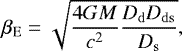
The theory of lensing by two-point-mass lenses is discussed in detail by Schneider & Weiss (1986). In the case of FRBs lensed by PBH binaries, we treat two PBHs as two point lenses. M = M1 + M2 is defined as the total mass of the lenses, where M1 and M2 are the masses of two separate lenses. Throughout the paper, we consider the case M1 = M2 = 30 M⊙ as an example. Then the Einstein radius is defined as
 (1)
(1)
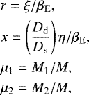
where Dd is the angular diameter distance from the lens to the observer, Ds is the angular diameter distance from the source to the observer, and Dds is the angular diameter distance between lens and source. We define the following dimensionless quantities
 (2)
(2)
where η is the position of the source in the source plane, and ξ is the position where light rays hit the lens plane.
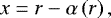
Given the position of the source, there are between three and five image positions. The positions of images in the lens plane are given bythe lens equation (Schneider & Weiss 1986),
 (3)
(3)
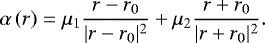
Lenses are located at the points βEr0 and − βEr0. r0 = (X, 0), where X ≥ 0 is the position of the lens on the lens plane.
With the positions of lenses, source and images, we can calculate the amplification factor I0 for every image, that is, the ratio of the flux density of one of the images caused by light deflection and the image when the lenses were absent
 (5)
(5)
The gravitational lensing time delay between two images ra, rb can be calculated from (Schneider & Weiss 1986)
![\begin{equation*}c\mathrm{\Delta} t=\beta_{\mathrm{E}}^{2}\frac{D_{\mathrm{s}}}{D_{\mathrm{d}}D_{\mathrm{ds}}}(1+z_{\mathrm{d}})[\mathrm{\Theta}({r_a},{x})-\mathrm{\Theta}({r_b},{x})], \end{equation*}](/articles/aa/full_html/2018/06/aa31160-17/aa31160-17-eq7.png) (7)
(7)
where Ψ(r) is the gravitational potential of the mass distribution and  , Dd is the angular diameter distance from the observer to the lens, Ds is the angular diameter distance from the observer to the source, and Dds is angular diameter distance from the lens to the source.
In order to find all of the image positions for any given source position, we follow the search routine for image positions proposed in Schneider & Weiss (1986). Firstly, we choose special starting point x0 which has image positions r0 solved using an analytical method. These starting points satisfy x01 = 0 or x02 = 0 where x0 = (x01, x02). Secondly, let x1 be a point near x0. The corresponding image positions of r1 are given by the differential lens equation, dx = Adr, that is,  . Thirdly, we insert
  into the lens Eq. (3) to find the corresponding source position
  . The condition is
  . If this condition is not satisfied, we take the next iterative step. For example, we use
  as starting points to do the next loop of calculation. Another thing to note is that any steps of the calculation should not cross a critical line, which is given by det A = 0. In order to find all image positions of a given source, we should choose suitable starting points in different areas separated by critical lines.
With a specific configuration of lenses and source, we require two conditions. Firstly, we should observe at least three images, that is, three peaks in the FRB light curve. The flux ratio I between every two images should be smaller thana critical flux ratio If. Secondly, there are at least three images which have the observed time delay between every two images larger than a critical time tf. Given the position of source and the distance of source and lenses, these conditions require the lens system to stay in some specific areas. We define these specific areas as the cross section σ. We use the Monte Carlo method to calculate the cross section.
The separation of two lenses could affect the cross section. We generate the PBH binaries and obtain the distribution of their separations using the mechanism proposed by Nakamura et al. (1997) and Sasaki et al. (2016). Then, given the distance of source and lenses, we calculate the average cross section by simply averaging the cross section of a large number of PBH binaries staying in this distance. Here, the average cross section σa (M, μ1, μ2, zs, zl) is a function of the total mass of the lenses M, mass ratios μ1 and μ2, redshift of source zs and lens system zl. We calculate the average cross section of lenses at different distances when the source is located at z = 0.5 as an example. The result is shown in Fig. 1.
Next wecalculate the lensing optical depth of a source, which indicates the probability that this source is lensed and the multi-peak structure is observable, at redshift zs from
 (8)
(8)
To obtain the estimated number of detected lensing events of FRBs by PBH binaries, we need to convolve the optical depth for a single FRB with the redshift distribution of FRBs. Similar to Muñoz et al. (2016) and Caleb et al. (2016), we discuss two redshift distributions of FRBs. The first one is a constant comoving number density, that is, ρ(z) = constant. Observations show that the host galaxy of FRB 121102 is a dwarf galaxy with low metallicity and prominent emission lines (Tendulkar et al. 2016), sharing similar properties with long gamma-ray bursts (GRBs). Meanwhile, long GRBs trace the star formation history (SFH; Wijers et al. 1998; Wanderman & Piran 2010; Wang et al. 2015). If FRB 121102 is typical of the wider FRB population, the rate of FRB would trace the SFH. So we also consider that FRB number density is proportional to the SFH. The SFH is (Hopkins & Beacom 2006)
 (9)
(9)
with a = 0.0170, b = 0.13, c = 3.3, and d = 5.3 and h = 0.7 (Cole et al. 2001; Wang 2013) is used. The comoving volume of a shell of width d z at redshift z is d V (z) = [4πχ2(z)∕H(z)]dz. Introducing the Gaussian cutoff to represent an instrumental signal-to-noise (S/N) threshold, we get the distribution of FRBs;
![\begin{equation*}N_{\mathrm{FRB}}(z)=\mathbb{N}_{\mathrm{FRB}}\frac{\rho(z)\chi(z)^{2}}{H(z)(1+z)}\mathrm{e}^{-d_{\mathrm{L}}^{2}/[2d_{\mathrm{L}}^{2}(z_{\mathrm{cut}})]}, \end{equation*}](/articles/aa/full_html/2018/06/aa31160-17/aa31160-17-eq16.png) (10)
(10)
where  is the normalizing factor and the term (1 + z) accounts for the effect of cosmologicaltime dilation. We choose Ωvac = 0.714, ΩM = 0.286, and H0 = 69.6 km s−1 Mpc−1 in our calculation.
Then we can calculate the integrated optical depth 
 (11)
(11)
Inter-channel dispersion will broaden the FRB pulse width. Meanwhile, its intrinsic pulse profile and scattering with the intergalactic medium will also contribute the total pulse width. Similar to Muñoz et al. (2016), we choose 1 and 0.1 ms as the critical times tf. For the critical flux ratio If, we adopt three different values, that is, 103, 100, and 10. The cutoff redshift is chosen as zcut = 0.5 (Muñoz et al. 2016), which fits the current FRB catalog well for both two distributions of FRBs. In Table 1, we show the integrated optical depth  for different fractions of dark matter f = 10−1, 10−2, 10−3 in PBHs for FRB number density proportional to SFH. In Table 2, we show
  for different f = 10−1, 10−2, 10−3 in PBHs for a constant FRB number density.
We choose the above values for tf and If because the duration time of FRBs is on the order of 1 ms1. Therefore, the choice of critical time tf = 1 ms is reasonable. We compare the repeating FRBs with the lensing FRBs since repeating FRBs also have multi-peak structures which might mix with the lensing FRBs. It turns out that the time interval between successive bursts for the repeating FRB 121102 is larger than several tens of seconds (Wang & Yu 2017). Therefore, the lensing FRBs can be discriminated from typicalrepeating FRBs. To date, multiple bursts have only been observed for the repeating FRB 121102. Fluxes are 670 mJy (Chatterjee et al. 2017) and 20 mJy (Spitler et al. 2016) for the brightest and dimmest burst, respectively, giving a flux ratio between them of about 33. Therefore, the choice of the critical flux ratio If is reasonable.
Since the integrated optical depth  is very small, the expected number of lensing FRBs by PBH binaries is
 (12)
(12)
Connor et al. (2016) estimated that the Canadian hydrogen intensity mapping experiment (CHIME) could detect about 104 FRBs per year. We could expect the detection of FRBs strongly lensed by PBH binaries. For example, the number of strongly lensed FRBs is about 36 for tf = 1 ms, If = 100 and f = 0.1 per year. Because most of the FRBs are below z = 1.5 in our calculation when choosing zcut = 0.5, the band of CHIME is not severely affected by redshift.
Integrated optical depth  for different parameters for a FRB number density proportional to SFH.
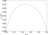 |
Fig. 1 Average cross section σa of lenses at different distances when the redshift of the source is z = 0.5 and the fraction of dark matter in PBHs is f = 0.1. The critical time tf = 0.1 ms and critical flux ratio If = 1000 are used. |
Integrated optical depth  for different parameters for a constant FRB comoving number density.
Results of the simulation of 2 × 10⁵ FRBs for different parameters.
3 Numerical simulations
We further simulate the gravitational lensing events of FRBs by PBH binaries to verify the analytical calculation in the above section. Assuming the distribution of PBH binaries is isotropic and uniform in space, we generate the PBH binaries following Sasaki et al. (2016). As mentioned in the previous section, we consider the distribution of FRBs following the SFH (Caleb et al. 2016). For the constant comoving number density, the difference of the simulation resulting from the SFH case is less than 30%.
We simulate 2 × 10⁵ FRBs for different fractions of dark matter f = 10−1, 10−2, 10−3 in PBHs, respectively. We choose Ωvac = 0.714, ΩM = 0.286, and H0 = 69.6 km s−1 Mpc−1 in our calculation. For each FRB, we consider the PBH binaries which could provide the strongest lensing effect. The lensing efficiency is indicated by lensing kernel
 (13)
(13)
which is proportional to DdsDd∕Ds (Sheldon 2002; Courbin & Minniti 2002). It describes the geometry of the lense-source system. A larger  indicates a stronger lensing effect. As an example, the lensing kernel of the lenses at different redshifts when the source is at redshift z = 1.3 is shown in Fig. 2. The distance of PBH binaries from the line of sight can also affect the lensing effect. Because the lensing events depend on other parameters, such as the orbital elements of the binaries, the strongest lensing event might not give the expected observable multi-peak FRBs. Meawhile, the magnification and time delay are also required. Therefore, we use several criteria to show the reliability of our results. We choose the PBH binaries by finding the smallest value of
  ,
,  or
or  , where θ is the angular distance of the PBH binary from the line of sight, and b is the linear distance of the PBH binary from the line of sight, that is, the impact parameter. We calculate the positions of images, time delay, and flux ratio of every second image. Then, we check whether they could conform with the conditions concerning time delay and flux ratio. We record all the lensing events with flux ratio I < 104 and time delay t > 0.5 × 10⁻⁴ s and give the results of the simulations in Table 3 for all three different ways of choosing PBH binaries. We find that the difference due to this latter choice is not obvious. Therefore, the choice of criteria cannot significantly affect the results. They all provide a lower limit of observable multi-peak FRBs. We further show the results for choosing PBH binaries by finding the smallest value of
  in Fig. 3. The number of lensing events is strongly influenced by the fraction of dark matter, f, critical time delay, tf, and critical flux ratio, If.
There are some differences between the analytical results in Sect. 2 and numerical simulations in Sect. 3. These differences are reasonable because we make some assumptions in the calculation in Sect. 2. For example, the average cross section used to calculate the optical depth is not very accurate. In Sect. 3, we use the Monte Carlo method to calculate the cross section since the allowed regions are not regular, as only a single lense is used.
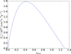 |
Fig. 2 Lensing kernel |

4 Discussion and conclusion
FRBs are promising tools to probe MACHOs. Firstly, FRBs are strong and short events, which means that they could serve as good candidates to probe the lensing events. As a result of lensing by black hole binaries, we should detect multi-peak FRBs. Since FRBs are strong and short, their multi-peak structure might be observable. Secondly, the rate of FRBs can be as high as a few thousand per day for the whole sky. Lastly, in the upcoming or ongoing surveys, the observation of a large number of FRBs is promising.
In this paper, we estimate the possibility of detecting lensing events of FRBs by PBH binaries. The typical time interval between different images is roughly 1 ms. The flux ratio between different images is from approximately 10 to 103. With an expected detection rate of FRBs by the upcoming experiment CHIME of 104 FRBs per year, we could expect five detections of multi-peak FRBs with time intervals larger than 1 ms and flux ratios less than 103 per year in the upcoming FRB surveys if the fraction of dark matter in MACHOs is f =0.01. If the lensing events are detected, we could analyze the structure of the peaks of FRBs to infer the separation and masses of two lenses to verify the primordial black hole scenario for gravitational-wave events. Alternatively, if no FRBs are lensed, the strongest constraints will be those put on the fraction of dark matter in the form of compact objects.
In our calculation, we use the formation mechanism of PBH binaries proposed in Nakamura et al. (1997). Tidal force from the nearby PBH provides the angular momentum of the PBH binaries. Bird et al. (2016) proposed that PBH binaries are formed due to the gravitational radiation when they pass by one another. We wish to point out that in our calculation, these two mechanisms do not have obvious differences. In the first mechanism, most of the PBH binaries will have an eccentricity very close to one. The movement of PBHs in the binary system could be very similar to movement when they are free. If we assume the same number density of PBHs, the results from two mechanisms would be very similar.
Cordes et al. (2017) claim that plasma lenses in FRB host galaxies can produce multiple bursts with different apparent strengths, arrival times, and dispersion measurements. There are several differences between our results and theirs. Firstly, the positions and “gain” (or amplification) of burst images are different for different frequencies in Cordes et al. (2017). However, in our discussion, the lensing effect caused by PBH binaries would be the same for any frequency. Secondly, the DMs of different images of bursts are different in their calculations. As for images caused by PBH lensing, the DMs of burst images contributed by the host galaxy are the same. Thirdly, their theory allows for the existence of larger time intervals between images, which could interpret the repeating FRB 121102 qualitatively. In our paper, we expect to distinguish between repeating FRBs and multiply imaged bursts caused by PBH binaries.
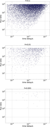 |
Fig. 3 Simulations of 2 × 10⁵ FRBs with different fractions of dark matter f = 10−1, 10−2, 10−3, respectively. All three panels show all the lensing events with flux ratio I < 104 and time delay t > 0.5 × 10⁻⁴ s. |
Acknowledgements
We thank the anonymous referee for constructive suggestions that have allowed us to improve our manuscript. This work is supported by the National Basic Research Program of China (973 Program, grant No. 2014CB845800) and the National Natural Science Foundation of China (grants 11422325 and 11373022), the Excellent Youth Foundation of Jiangsu Province (BK20140016).
References
- Abbott, B. P., Abbott, R., Abbott, T. D., et al. 2016a, Phys. Rev. Lett., 116, 061102 [Google Scholar]
- Abbott, B. P., Abbott, R., Abbott, T. D., et al. 2016b, Phys. Rev. Lett., 116, 241103 [Google Scholar]
- Alcock, C., Allsman, R. A., Alves, D. R., et al. 2001, ApJ, 550, 169 [NASA ADS] [CrossRef] [Google Scholar]
- Ali-Haïmoud, Y., & Kamionkowski, M. 2017, Phys. Rev. D, 95, 043534 [NASA ADS] [CrossRef] [Google Scholar]
- Arvanitaki, A., Baryakhtar, M., Dimopoulos, S., Dubovsky, S., & Lasenby, R. 2017, Phys. Rev. D, 95, 043001 [NASA ADS] [CrossRef] [Google Scholar]
- Bandura, K., Addison, G. E., Amiri, M., et al. 2014, Proc. SPIE, 9145, 914522 [CrossRef] [Google Scholar]
- Belczynski, K., Holz, D. E., Bulik, T., & O’haughnessy, R. 2016, Nature, 534, 512 [NASA ADS] [CrossRef] [Google Scholar]
- Belotsky, K. M., Dmitriev, A. E., Esipova, E. A., et al. 2014, Mod. Phys. Lett. A, 29, 1440005 [NASA ADS] [CrossRef] [Google Scholar]
- Bird, S., Cholis, I., Muñoz, J. B., et al. 2016, Phys. Rev. Lett., 116, 201301 [NASA ADS] [CrossRef] [Google Scholar]
- Caleb, M., Flynn, C., Bailes, M., et al. 2016, MNRAS, 458, 718 [NASA ADS] [CrossRef] [Google Scholar]
- Carr, B. J. 1975, ApJ, 201, 1 [Google Scholar]
- Carr, B. J. 1976, ApJ, 206, 8 [NASA ADS] [CrossRef] [Google Scholar]
- Carr, B. J., & Hawking, S. W. 1974, MNRAS, 168, 399 [NASA ADS] [CrossRef] [MathSciNet] [Google Scholar]
- Chatterjee, S., Rodriguez, C. L., & Rasio, F. A. 2017, ApJ, 834, 68 [NASA ADS] [CrossRef] [Google Scholar]
- Cholis, I., Kovetz, E. D., Ali-Haïmoud, Y., et al. 2016, Phys. Rev. D, 94, 084013 [NASA ADS] [CrossRef] [Google Scholar]
- Cole, S., Norberg, P., Baugh, C. M., et al. 2001, MNRAS, 326, 255 [NASA ADS] [CrossRef] [Google Scholar]
- Connor, L., Lin, H. H., & Masui, K. 2016, MNRAS, 460, 1054 [NASA ADS] [CrossRef] [Google Scholar]
- Cordes, J. M., Wasserman, I., Hessels, J. W. T., et al. 2017, ApJ, 842, 35 [NASA ADS] [CrossRef] [Google Scholar]
- Courbin, F., & Minniti, D. 2002, Gravitational Lensing: An Astrophysical Tool (Berlin: Springer Science & Business Media) [CrossRef] [Google Scholar]
- Dai, Z. G., Wang, J. S., Wu, X. F., & Huang, Y. F. 2016, ApJ, 829, 27 [NASA ADS] [CrossRef] [Google Scholar]
- Falcke, H., & Rezzolla, L. 2014, A&A, 562, A137 [NASA ADS] [CrossRef] [EDP Sciences] [Google Scholar]
- Frampton, P. H., Kawasaki, M., Takahashi, F., & Yanagida, T. T. 2010, JCAP, 04, 023 [NASA ADS] [CrossRef] [Google Scholar]
- García-Bellido, J., Linde, A., & Wands, D. 1996, Phys. Rev. D, 54, 6040 [NASA ADS] [CrossRef] [Google Scholar]
- Hartwig, T., Volonteri, M., Bromm, V., et al. 2016, MNRAS, 460, L74 [NASA ADS] [CrossRef] [Google Scholar]
- Hopkins, A. M., & Beacom, J. F. 2006, ApJ, 651, 142 [NASA ADS] [CrossRef] [MathSciNet] [Google Scholar]
- Hosokawa, T., Hirano, S., Kuiper, R., et al. 2016, ApJ, 824, 119 [NASA ADS] [CrossRef] [Google Scholar]
- Inayoshi, K., Kashiyama, K., Visbal, E., & Haiman, Z. 2016, MNRAS, 461, 2722 [NASA ADS] [CrossRef] [Google Scholar]
- Khlopov, M. Y. 2010, Res. Astron. Astrophys., 10, 495 [NASA ADS] [CrossRef] [Google Scholar]
- Lorimer, D. R., Bailes, M., McLaughlin, M. A., Narkevic, D. J., & Crawford, F. 2007, Science, 318, 777 [NASA ADS] [CrossRef] [PubMed] [Google Scholar]
- Mandic, V., Bird, S., & Cholis, I. 2016, Phys. Rev. Lett., 117, 201102 [NASA ADS] [CrossRef] [Google Scholar]
- Mediavilla, E., Muñoz, J. A., & Falco, E., et al. 2009, ApJ, 706, 1451 [NASA ADS] [CrossRef] [Google Scholar]
- Mészáros, P. 1975, A&A, 38, 5 [NASA ADS] [Google Scholar]
- Mink, S. E., & Mandel, I. 2016, MNRAS, 460, 3545 [NASA ADS] [CrossRef] [Google Scholar]
- Monroy-Rodríguez, M. A., & Allen, C. 2014, ApJ, 790, 159 [NASA ADS] [CrossRef] [Google Scholar]
- Muñoz, J. B., Kovetz, E. D., Dai, L., & Kamionkowski, M. 2016, Phys. Rev. Lett., 117, 091301 [NASA ADS] [CrossRef] [Google Scholar]
- Nakamura, T., Sasaki, M., Tanaka, T., & Thorne, K. S. 1997, ApJ, 487, 139 [NASA ADS] [CrossRef] [Google Scholar]
- Newburgh, L. B., Bandura, K., Bucher, M. A., et al. 2016, SPIE Conf. Ser., 9906, 99065X [Google Scholar]
- Pooley, D., Rappaport, S., Blackburne, J., et al. 2009, ApJ, 697, 1892 [NASA ADS] [CrossRef] [Google Scholar]
- Quinn, D. P., Wilkinson, M. I., Irwin, M. J., et al. 2009, MNRAS, 396, 11 [Google Scholar]
- Raccanelli, A., Kovetz, E. D., Bird, S., et al. 2016, Phys. Rev. D, 94, 023516 [NASA ADS] [CrossRef] [Google Scholar]
- Ricotti, M. 2007, ApJ, 662, 53 [NASA ADS] [CrossRef] [Google Scholar]
- Ricotti, M., Ostriker, J. P., & Mack, K. J. 2008, ApJ, 680, 829 [NASA ADS] [CrossRef] [Google Scholar]
- Rodriguez, C. L., Chatterjee, S., & Rasio, F. A. 2016a, Phys. Rev. D, 93, 084029 [NASA ADS] [CrossRef] [Google Scholar]
- Rodriguez, C. L., Haster, C. J., Chatterjee, S., et al. 2016b, ApJ, 824, L8 [NASA ADS] [CrossRef] [Google Scholar]
- Sasaki, M., Suyama, T., Tanaka, T., et al. 2016, Phys. Rev. Lett., 117, 061101 [NASA ADS] [CrossRef] [Google Scholar]
- Schneider, P., & Weiß, A. 1986, A&A, 164, 237 [NASA ADS] [Google Scholar]
- Schutz, K., & Liu, A. 2017, Phys. Rev. D, 95, 023002 [NASA ADS] [CrossRef] [Google Scholar]
- Sheldon, E. S. 2002, PhD Thesis, University of Michigan, USA [Google Scholar]
- Spitler, L. G., Scholz, P., Hessels, J. W. T., et al. 2016, Nature, 521, 202 [NASA ADS] [CrossRef] [Google Scholar]
- Tendulkar, S. P., Bassa, C. G., Chatterjee, S., et al. 2017, ApJ, 834, L7 [NASA ADS] [CrossRef] [Google Scholar]
- Thornton, D., Stappers, B., Bailes, M., et al. 2013, Science, 341, 53 [NASA ADS] [CrossRef] [PubMed] [Google Scholar]
- Totani, T. 2013, PASJ, 65, L12 [NASA ADS] [CrossRef] [Google Scholar]
- Tisserand, P., Guillou, L. L., Afonso, C., et al. 2007, A&A, 469, 387 [NASA ADS] [CrossRef] [EDP Sciences] [Google Scholar]
- Verheijen, M. A. W., Oosterloo, T. A., van Cappellen, W. A., et al. 2008, AIP Conf. Proc., 1035, 265 [Google Scholar]
- Wanderman, D., & Piran, T. 2010, MNRAS, 406, 1944 [NASA ADS] [Google Scholar]
- Wang, F. Y. 2013, A&A, 556, A90 [NASA ADS] [CrossRef] [EDP Sciences] [Google Scholar]
- Wang, F. Y., & Yu, H. 2017, JCAP, 03, 023 [NASA ADS] [CrossRef] [Google Scholar]
- Wang, F. Y., Dai, Z. G., & Liang, E. W. 2015, New Astron. Rev., 67, 1 [NASA ADS] [CrossRef] [Google Scholar]
- Wang, J. S., Yang, Y. P., Wu, X. F., Dai, Z. G., & Wang, F. Y. 2016, ApJ, 822, L7 [NASA ADS] [CrossRef] [Google Scholar]
- Wijers, R. A. M. J., Bloom, J. S., Bagla, J. S., et al. 1998, MNRAS, 294, L13 [NASA ADS] [CrossRef] [Google Scholar]
- Woosley, S. E. 2016, ApJ, 824, L10 [NASA ADS] [CrossRef] [Google Scholar]
- Wyrzykowski, L., Skowron, J., Kozlowski, S., et al. 2011, MNRAS, 416, 2949 [NASA ADS] [CrossRef] [EDP Sciences] [Google Scholar]
- Yoo, J., Chaname, J., & Gould, A. 2004, ApJ, 601, 311 [NASA ADS] [CrossRef] [Google Scholar]
- Yu, H., & Wang, F. Y. 2017, A&A, 660, A3 [NASA ADS] [CrossRef] [EDP Sciences] [Google Scholar]
- Yu, Y.-W., Cheng, K.-S., Shiu, G., & Tye, H. 2014, JCAP, 11, 040 [NASA ADS] [CrossRef] [Google Scholar]
- Zhang, B. 2014, ApJ, 780, L21 [NASA ADS] [CrossRef] [Google Scholar]
- Zhang, B. 2016, ApJ, 827, L31 [NASA ADS] [CrossRef] [Google Scholar]
All Tables
Integrated optical depth for different parameters for a FRB number density proportional to SFH.
Integrated optical depth for different parameters for a constant FRB comoving number density.
All Figures
|
Fig. 1 Average cross section σa of lenses at different distances when the redshift of the source is z = 0.5 and the fraction of dark matter in PBHs is f = 0.1. The critical time tf = 0.1 ms and critical flux ratio If = 1000 are used. |
| In the text | |
|
Fig. 2 Lensing kernel |
| In the text | |
|
Fig. 3 Simulations of 2 × 10⁵ FRBs with different fractions of dark matter f = 10−1, 10−2, 10−3, respectively. All three panels show all the lensing events with flux ratio I < 104 and time delay t > 0.5 × 10⁻⁴ s. |
| In the text | |
Current usage metrics show cumulative count of Article Views (full-text article views including HTML views, PDF and ePub downloads, according to the available data) and Abstracts Views on Vision4Press platform.
Data correspond to usage on the plateform after 2015. The current usage metrics is available 48-96 hours after online publication and is updated daily on week days.
Initial download of the metrics may take a while.