| Issue |
A&A
Volume 614, June 2018
|
|
|---|---|---|
| Article Number | A54 | |
| Number of page(s) | 9 | |
| Section | The Sun | |
| DOI | https://doi.org/10.1051/0004-6361/201630067 | |
| Published online | 12 June 2018 | |
LOFAR observations of the quiet solar corona
1
Leibniz-Institut für Astrophysik Potsdam,
An der Sternwarte 16,
14482
Postdam,
Germany
e-mail: This email address is being protected from spambots. You need JavaScript enabled to view it.
2
RAL Space, Science & Technology Facilities Council, Rutherford Appleton Laboratory,
Harwell Campus,
Oxford,
Oxfordshire
OX11 0QX,
UK
3
Space Radio-Diagnostics Research Centre, University of Warmia and Mazury,
Olsztyn,
Poland
4
ASTRON, Netherlands Institute for Radio Astronomy,
Postbus 2,
7990,
AA Dwingeloo,
The Netherlands
5
School of Physics, Trinity College Dublin,
Dublin 2,
Ireland
6
Solar-Terrestrial Center of Excellence - SIDC, Royal Observatory of Belgium,
Av. Circulaire 3,
180
Brussels,
Belgium
7
Commission for Astronomy, Austrian Academy of Sciences,
Schmiedlstrasse 6,
8042
Graz,
Austria
Received:
15
November
2016
Accepted:
20
February
2018
Abstract
Context. The quiet solar corona emits meter-wave thermal bremsstrahlung. Coronal radio emission can only propagate above that radius, Rω, where the local plasma frequency equals the observing frequency. The radio interferometer LOw Frequency ARray (LOFAR) observes in its low band (10–90 MHz) solar radio emission originating from the middle and upper corona.
Aims. We present the first solar aperture synthesis imaging observations in the low band of LOFAR in 12 frequencies each separated by 5 MHz. From each of these radio maps we infer Rω, and a scale height temperature, T. These results can be combined into coronal density and temperature profiles.
Methods. We derived radial intensity profiles from the radio images. We focus on polar directions with simpler, radial magnetic field structure. Intensity profiles were modeled by ray-tracing simulations, following wave paths through the refractive solar corona, and including free-free emission and absorption. We fitted model profiles to observations with Rω and T as fitting parameters.
Results. In the low corona, Rω < 1.5 solar radii, we find high scale height temperatures up to 2.2 × 10⁶ K, much more than the brightness temperatures usually found there. But if all Rω values are combined into a density profile, this profile can be fitted by a hydrostatic model with the same temperature, thereby confirming this with two independent methods. The density profile deviates from the hydrostatic model above 1.5 solar radii, indicating the transition into the solar wind.
Conclusions. These results demonstrate what information can be gleaned from solar low-frequency radio images. The scale height temperatures we find are not only higher than brightness temperatures, but also than temperatures derived from coronograph or extreme ultraviolet (EUV) data. Future observations will provide continuous frequency coverage. This continuous coverage eliminates the need for local hydrostatic density models in the data analysis and enables the analysis of more complex coronal structures such as those with closed magnetic fields.
Key words: Sun: corona / Sun: radio radiation / waves / solar wind
© ESO 2018
1 Introduction
Radio observations of the Sun at frequencies below 100 MHz probe the middle and upper corona, since radio waves cannot propagate through regions where the wave frequency is lower than the local plasma frequency,  , with electron number density, Ne, elementary charge, e, electron mass, me, and vacuum permittivity, ϵ0. For 100 MHz, this corresponds to a maximum density of Ne = 1.2 × 10¹⁴ m−3, that is generally exceeded in the lower corona. Interferometric imaging observations at low frequencies are well suited for gaining insights into upper coronal structures. This technique has been used over many decades.
Wild (1970) observed the Sun with the Culgoora radio telescope at 80 MHz and determined flare positions, and also studied the quiet solar radio emission and found brightness temperatures mostly below 106 K. Culgoora data were also used by Dulk et al. (1977) for coronal hole studies. These authors combined the data with microwave and extreme ultraviolet (EUV) observations to constrain analytical transition region and coronal models. Kundu et al. (1983) observed the Sun with the Clark Lake telescope between 100 and 39 MHz, and found generally good agreement between radio maps and white-light coronograph images (Kundu et al. 1987). Wang et al. (1987) used this instrument to observe coronal holes and found brightness temperatures of not more than 7 × 10⁵ K at the solar disk center at 73.8 MHz. Ramesh et al. (2010) studied coronal streamers and tried to determine magnetic fields in these streamers with the Gauribidanur Radioheliograph (Ramesh et al. 1998). The Nançay Radioheliograph (NRH; Kerdraon & Delouis 1997) covers higher frequencies between 150 and 450 MHz, and has been used, for example, by Lantos (1999) to study medium- and large-scale features in the quiet solar corona, such as coronal holes.
The interpretation of radio images of the solar corona requires modeling of refractive effects, since the refractive index of a plasma approaches zero for plasma wave frequencies near the local plasma frequency, ωp. Alissandrakis (1994) calculated brightness temperature maps for simple coronal hole models based on ray-tracing calculations that consider refraction and opacity effects. The comparison of the model results with NRH data leads to the conclusion that knowledge of coronal structures is important for the interpretation of radio maps. A recent review by Shibasaki et al. (2011), covering wavelength ranges from millimeter to meter waves, also highlighted the importance of improved modeling of refraction and scattering effects in the solar corona.
Mercier & Chambe (2015) collected NRH data over one solar cycle and derived coronal density and temperature models in equatorial and polar directions. These authors found brightness temperatures around 6 × 10⁵ K at the lowest frequency of 150 MHz, but much higher scale height temperatures, around 1.6 × 10⁶ K in the equatorial and up to 2.2 × 10⁶ K in the polar direction.
The LOw Frequency ARray (LOFAR; van Haarlem et al. 2013) is a novel radio interferometer that observes the sky in two frequency bands of 10–90 MHz (low band) and 110–250 MHz (high band). The LOFAR telescope consists of a central core of 24 antenna stations within a 3 km × 2 km area near Exloo, the Netherlands, 14 remote stations spread over the Netherlands, and international stations in France, Germany, Ireland, Poland, Sweden, and the UK. The LOFAR baselines extend from tens of meters in the core up to 1550 km across Europe. With this setup, LOFAR combines a high angular resolution below 1″ with a large collecting area and thus high sensitivity.
As a versatile radio telescope, it has uses in many fields of radio astronomy. Science from LOFAR is organized around key science projects (KSPs). One of the KSPs is Solar Physics and Space Weather with LOFAR (Mann et al. 2011), which studies all aspects of the active Sun and its effects on interplanetary space, including the space environment of the Earth, which are commonly referred to as space weather.
The frequency range of LOFAR covers the middle (high band) and upper (low band) corona. However, scattering of radio waves on coronal turbulence prevents the arc-second resolution provided by international baselines. Mercier et al. (2015) reported minimum source sizes of 31″ at 327 MHz and 35″ at 236 MHz. So, the angular resolution of solar imaging with LOFAR is restricted to several tens of arc-seconds at best. For LOFAR frequencies, this corresponds to maximum baseline lengths of a few 10 km. Such baselines are provided by the LOFAR core and the nearest remote stations.
Previous work on solar observations with LOFAR has focused on the active Sun, for example, studies of type III radio bursts (Morosan et al. 2014). Here, we present quiet-Sun observations in the low band on multiple frequencies between 25 and 79 MHz. A ray-tracing method is presented that is used to reproduce observed intensity profiles with coronal density and scale height temperature as model parameters. As the different frequencies probe different layers of the solar corona, these results can be used to construct coronal density and temperature profiles, at lower frequencies, i.e., larger heights, than most of the earlier works presented above.
2 LOFAR low-band images of the quiet Sun
The appearance of the radio Sun can change within seconds, especially during solar radio bursts. Therefore, solar imaging with LOFAR is normally snapshot imaging with a short integration time of 1 s, or even 0.25 s, to capture the dynamics of solar radio bursts. But for quiet-Sun studies, Earth rotation aperture synthesis can be used to improve uv coverage, i.e., taking advantage of the rotation of the Earth to increase the variety of different baseline lengths and orientations of the interferometric array.
2.1 External calibration with Tau A
The structure of the radio Sun is a priori unknown and can vary substantially with time. The thermal background emission from the 106 K hot corona can be estimated easily, but the intensity of solar radio bursts can exceed this by up to four orders of magnitude (Mann 2010). Nonthermal radio emission from active regions, including radio bursts, can appear as compact or extended sources with unknown intensities somewhere on the solar disk or even off the limb. Measuring their position relative to the Sun is important for the interpretation of the physical processes in the solar corona, since this measurement enables an alignment with observations in other wavelength ranges such as optical, EUV, or X-rays.
This precludes the use of a pure self-calibration approach, which is based on an initial sky model with some prescribed solar intensity and center of brightness. Therefore, an external calibration source is needed both for amplitude and phase calibration. This needs to be a strong source to prevent the active Sun from interfering with it easily. During the commissioning phase of LOFAR, Tau A was found to be a suitable calibrator, which can be used from late spring until the end of August. During the solar observations, another LOFAR beam was pointed toward Tau A, recording calibration data on the same frequencies as for the Sun.
However, one caveat needs to be taken into consideration for these observations on 8 August: Tau A is located about 50° west of the Sun at this time of the year, so it sinks toward the horizon during the observing period of 8 h, centered around local noon. Hence its radio signal has to traverse a longer path through the atmosphere, including the ionosphere. The intensity of the Tau A signal decreases in the second half of the observing period. Since Tau A is also used for amplitude calibration, a spurious intensity increase would be transferred to the Sun.
Therefore, we use only the first 3 h of observing time from 08:02 UT to 11:02 UT. Figure 1 shows the uv coverage for both the usual snapshot solar imaging, and for the 3 h used here for aperture synthesis imaging of the quiet Sun. The uv coverage is improved substantially.
The Tau A data are calibrated with LOFAR’s standard BlackBoard Selfcal (BBS) system (van Haarlem et al. 2013). The solution wasrestricted to longer baselines above 150 wavelengths, since Tau A is a relative compact object with a strong signal on those baselines, while the Sun is a more extended object with most intensity in shorter baselines. This approach reduces the risk of solar interference in the Tau A data used for calibration, and still provides phase and amplitude corrections for all LOFAR stations.
2.2 Low-frequency solar images
After calibration of Tau A, the solutions are transferred to the solar data. Imaging was performed using the Solar Imaging Pipeline (Breitling et al. 2015), taking the movement of the Sun with respect to the background sky into consideration. To estimate thequality of the LOFAR images, it is useful to compare these images with NRH data, although these are obtained at higher frequencies.
Figure 2 shows images of the Sun from the NRH at their lowest observing frequency of 150.9 MHz, and an EUV image taken by the Solar Dynamics Observatory (SDO) in the Fe IX line at 171Å. Both images were taken in the morning hours of 8 August 2013. The SDO picture has been taken at 9:15 UT, i.e., during the LOFAR integration time. This image shows active regions along the solar equator with some more activity in the southern hemisphere. The Nançay image is from 11:30 UT; earlier images had strong artifacts. This image shows the quiet coronawith slightly higher radio intensity south and east of the equator. There was no burst activity during the LOFAR observing time.
Figure 3 shows the LOFAR solar images for all observed frequencies. Imaging was restricted to maximum baseline lengths of 2500 wavelengths, λ, since longer baselines provide little useful information from coronal scattering, but could add noise to the images. The corresponding array beams are indicated by small ellipses in the upper right corners of each image. Their shapes are frequency dependent because a given baseline in the LOFAR array, with given length (in km), can correspond to less than 2500 λ for lower, and more than 2500 λ for higher frequencies. As the uv coverage is relatively sparse (see Fig. 1), such a removal of a baseline from one frequency tothe next can visibly alter the beam shape.
The quiet-Sun image at 79 MHz is in good agreement with the Nançay image, although the frequency is lower by almost a factor two. Both show the same structure with slightly enhanced emission toward the southeast of the disk center. The images change very little for the next lower frequencies, although the center of brightness moves a bit to the solar center. Below 50 MHz, it becomes evident that the solar diameter increases with decreasing frequency. The image quality starts to deteriorate below 34 MHz. It is still useful at 30 MHz, but very poor for 25 MHz. The lowest frequency of 19 MHz is not shown in Fig. 3 because too much radio frequency interference (RFI) prevented us from obtaining any useful images.
There can be many reasons for the lower image quality at lower frequencies. One reason is an increasing RFI background, another is that ionospheric influences are not fully corrected when solutions are transferred from the 50° separated Tau A, which is observed through a different part of the ionosphere. This becomes more severe as the observing frequency approaches the ionospheric cutoff.
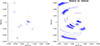 |
Fig. 1 uv coverage of the solar observations for snapshot imaging (left) and an observing time of 3 h (right). |
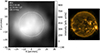 |
Fig. 2 Nançay Radioheliograph image at 150.9 MHz (left), and EUV image from the Solar Dynamics Observatory (SDO) in the Fe IXline at 171 Å (right). |
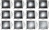 |
Fig. 3 Images of the Sun from LOFAR from 8 August 2013, 08:02–11:02 UT, for several low-band frequencies ranging from 25 to 79 MHz. |
2.3 Polar and equatorial intensity profiles
It is evident that the images in Fig. 3 do not show solar disks with relatively constant intensity and a well-defined limb, but maxima near the image centers and gradual intensity decrease with increasing angular distance, α, from the centers. Intensity profiles can be derived from the images as a function of α for each position angle. Averaging over all position angles reduces the image noise and provides smoother profiles, but polar and equatorial regions should be distinguished. The SDO image in Fig. 2 shows an activity belt around the solar equator, and a more radial magnetic field configuration around the poles. Closed magnetic field lines near the equator could lead to a slower decrease of plasma density with height than at higher latitudes.
Figure 4 shows the position-angle averaged intensity profiles within 30° from the polar (north–south) and equatorial (east–west) directions, as derived from the LOFAR image for 74 MHz. It can be clearly seen that the intensity indeed falls off more rapidly in the polar direction, which corresponds to an elongated appearance of the radio Sun inthe equatorial direction. This asymmetry is not too pronounced, which is typical for the solar maximum, but the corona is not radially symmetric.
These results are in agreement with the analysis of Mercier & Chambe (2015), who studied NRH images of the quiet Sun at frequencies between 150 and 450 MHz, and also found that the radio Sun generally is more extended in the east-west than in the north-south direction.
The intensity values in Fig. 4 are converted from Jy beam−1 to brightness temperatures, using the beam sizes indicated by small ellipses in Fig. 3 and the Rayleigh–Jeans law. The maximum brightness temperature near the disk center is close to 106 K. This is significantly higher than the coronal brightness temperatures around 7 × 10⁵ K usually found by other observers (Mercier & Chambe 2015; Lantos 1999; Wang et al. 1987; Dulk et al. 1977). However, the amplitude calibration of the LOFAR data is based on solution transfer from the relatively far away Tau A, as discussedabove. Different ionospheric conditions for the solar and calibrator beams could account for this difference.
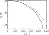 |
Fig. 4 Brightness temperature profiles derived from the 74 MHz image for polar (solid line) and equatorial (dashed line) regions. |
3 Radio emission from the quiet Solar corona
The radio images of the Sun in Fig. 3 appear bigger for lower frequencies. This is a well-known and expected behavior. Ina plasma, radio waves cannot propagate with a frequency that is less than the local plasma frequency, ωp. The plasma frequency only depends on the electron density, Ne, and on no other plasma parameters. In the approximately hydrostatic solar corona, the density increases toward the Sun. Therefore, a radio wave with frequency ω can only propagate in the corona, and reach an observer on Earth, above that coronal height where the electron density, Ne, equals ω2 me ϵ0∕e2. In other words, the plasma frequency defines a surface in the corona above which radio waves can escape. This radius is denoted as Rω.
Since the solar corona is highly structured, this surface is generally not a sphere. The density in, for example, a coronal hole is lower than in the rest of the corona, such that a given plasma frequency is found closer to the Sun. However, the density above active regions is higher, such that the same plasma frequency is found higher up in the corona. If closed coronal loops with higher density are present, the surface can be topologically more complex.
Radio emission from this surface is strongly influenced by refraction and optical thickness variation in the corona (Smerd 1950), which leads to the observed gradually decreasing intensity profiles in Fig. 4. In the remainder of this paper, we investigate how such intensity profiles are formed, and demonstrate how information on the coronal structure can be derived from these profiles. We only discuss the density profiles in the polar regions, since they show a simpler, radially outward magnetic-field geometry for larger α > 340″, as indicated by the EUV image in Fig. 2. Since coronal radio wave ray paths are refracted away from the solar disk center (see Fig. 5 in the next subsection), they traverse only these radial magnetic fields for α > 340″.
A polar, i.e., north–south, profile could be influenced by the equatorial activity belt for small α < 340″. However, the polar and equatorial intensity profiles in Fig. 4 hardly differ there. Both show the same slow intensity decrease from the maximum at the disk center, which continues up to α = 900″, where both profiles start deviating. This is far away from the equatorial activity belt for the polar profile. Therefore, closed magnetic field structures near the equator should have no significant influence on the following analysis of polar intensity profiles.
3.1 Radio wave refraction in the corona
In the solar corona, the electron cyclotron frequency is usually much smaller than the plasma frequency. Therefore, the refractive index of a radio wave can be described by that in a nonmagnetic plasma, 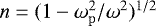 . It approaches zero for ω → ωp, so that radio waves can experience total reflection in the corona. This has important consequences for the appearance of the radio Sun as it is observed from Earth.
Figure 5 shows the geometry of radio wave refraction within the solar corona. The observer is located at the far right and looks into a direction that differs from the solar center by an angle α. This idealized picture is based on the assumption of a spherically symmetric solar corona.
We note that the line of sight can only reach Rω, i.e., the coronal height where ω = ωp, for observations of the centerof the solar disk. For α > 0, the ray pathis deflected at a larger coronal height. Such trajectories of meter waves through the corona were already discussed by Newkirk (1961) and reviewed by McLean & Melrose (1985).
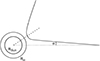 |
Fig. 5 Geometry of radio wave refraction in the solar corona. |
3.2 Appearance of the quiet radio Sun to the observer
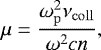
The thermal emission from the quiet radio Sun is free-free radiation with emissivity ϵ. The intensity i(α) seen in direction α corresponds to its line integral along the ray path for the optically thin limit. But the solar corona cannot be considered as optically thin, the absorption of radio waves in the plasma also has to be considered. According to McLean & Melrose (1985), it can be calculated as
 (1)
(1)
with collisional frequency  for Ne in m −3, Te in K, and observing frequency f = ω∕(2π) in Hz. The absorption length scale can be as short as 0.1 R⊙ for the coronal densities and temperatures discussed in this paper.
Emissivity, ϵ, and absorption, μ, are coupled through Kirchhoff’s Law,
 (2)
(2)
When a line integral along a ray path as that in Fig. 5 is calculated, the change of the refractive index along the path also needs to be taken into consideration. The intensity then evolves according to the radiative transfer equation (e.g., McLean & Melrose 1985)
 (3)
(3)
Such a ray-tracing simulation requires a coronal-density model for calculating not only the emission and absorption, but also the refractive index, which determines the ray path by means of Snell’s law, and enters Eq. (3) directly. As a simple approximation, we use a hydrostatic density model, which describes the coronal density, or the electron density, as
 (4)
(4)
with a parameter
 (5)
(5)
which contains the pressure scale height as the first factor, R⊙ is the solar radius, g⊙ = 274 m s−2 is the gravitational acceleration at the coronal base, and 0.6 proton masses is the average particle mass in the corona (Priest 1982). The temperature, T, is a scale height temperature determined by both electron and ion temperatures.
Nω = ω2meϵ0∕e2 is the density, where the plasma frequency equals the observing frequency, ω. In other words, Nω = Ne(Rω). Then the density around Rω can be written as
 (6)
(6)
Such a description has the advantage that a global density model for the whole corona is not required. Only the relative density decrease above Rω, with a scale height temperature, T, is needed.
Therefore a ray-tracing simulation for given observing frequency, ω, and angle α, depends on two model parameters, Rω and a coronal scale height temperature, T. This should be the temperature near Rω, since both emission and absorption are strongest at the lowest point of the ray path through the corona (see Fig. 5), which is near Rω and where the density is highest.
Integrating Eq. (3) along the ray path is now a two-step process. At first, the ray path needs to be determined, starting at the position of the observer 1 AU away from the Sun, and proceeding into direction α. The density model, Eq. (6), provides the refractive index, which leads to the ray path by Snell’s Law, all the way toward the Sun, through the corona, and back into interplanetary space. The ray path is calculated for a solar distance up to 1 AU.
The second step is integrating Eq. (3) back from interplanetary space beyond the Sun, through the corona, toward the observer. The initial condition is i = 0, i.e., it is assumed that no emission is coming from beyond that point. Since the emissivity scales with  , and the solar wind density at 1 AU is at least by a factor of 10−8 lower than that in the lower corona, the arbitrary choice of a starting point of 1 AU behind the Sun is not critical.
Figure 6 shows the results of such simulations for two different values of Rω. The other simulation parameters, i.e., a coronal scale height temperature T = 1.4 × 10⁶ K and an observing frequency f = 54 MHz, are identical. The electron temperature, Te, which enters Eq. (3), is set to be equal to the scale height temperature, T.
This is just the simplest approach to such a model. In general, T and Te can differ, for example, Mercier & Chambe (2015) deduced a much lower Te =6.2 × 10⁵ K. In the optically thick limit, i.e., small α near the disk center, Te determines the brightness temperature. In the optically thin limit, i.e., large α traversing the outer corona, the intensity, Eq. (3), is just a line integral over the emissivity ϵ, Eq. (2), which contains a factor  . In this case, the slope of an intensity curve in a semi-logarithmic plot such as Fig. 6 is independent of Te. For Rω = 1.5 R⊙ and α = 1500″, the optical depth τ = 0.2. For α =2000″, it has decreased to τ = 0.05. Thus the choice of Te is not critical for the larger α in Fig. 6, where the intensity profiles show a strong Rω dependence.
It follows from Fig. 6 that the radial extent of the radio Sun increases with higher Rω. This is not surprising, since a higher Rω just means that the sphere around the Sun, within which radio waves with frequency ω cannot propagate, is larger.
A radius of 1.5 R⊙ appears under an angle α = 1350″ to an observer on Earth. But the intensity values fall already for much smaller α below their peak value at the solar disk center. The same behaviors as those in Fig. 4 are found in observed intensity profiles. The reason for this lies in the ray path, as depicted in Fig. 5. For increasing α, the turning point of the ray path tends to be at a larger coronal height, where the plasma density and therefore the emissivity is lower.
The plotof this closest distance, Rmin, as a function of α in Fig. 7 confirms this conjecture. For higher α, the ray path probes only higher parts of the corona. For α = 1350″, Rmin has increased to 1.7 R⊙ from the original 1.5 R⊙ for α =0. For a coronal temperatureof 1.4 × 10⁶ K this corresponds to 0.8 pressure scale heights at altitudes around 1.6 R⊙. Since the emissivity of quiet-Sun radio emission scales with  , and the corona is not optically thick for these radio waves, this explains why both observed (Fig. 4) and model (Fig. 6) intensity profiles decrease for relatively small α.
The ray-tracing simulations depend not only on Rω, but also onthe coronal temperature. Intensity profiles for three different T are plotted in Fig. 8. Generally, the higher the scale height temperature, the further out the radio Sun extends. The slope of the intensity profile becomes temperature dependent for higher α >1200″, it decreases with increasing T. But, unlike the variation of Rω in Fig. 6, there is little influence of T on the intensity profile for lower α.
The reason for this also lies in the α dependence of the ray-path geometry. For higher α, the ray pathtraverses only higher parts of the corona (see Fig. 7). It follows from Eq. (6) that further away from Rω, the pressure scale height, and thus T, has an increasing impact on the plasma density there, and thus on both the free-free radio wave emission/absorption and the actual ray path.
The discussion of Figs. 6 and 8 leads to the conclusion that the ray-tracing simulation parameters Rω and T influence the resulting intensity profiles across the radio Sun in distinct ways. Therefore, it is possible to fit both of these to an observed intensity profile. Since the ray-tracing profiles coincide for smaller α <500″, it is the larger α that determine the fitting parameters. This has the consequence that the slightly enhanced emission south and, especially for the higher frequencies, east of the disk center found in Fig. 3 does not influence the results.
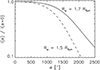 |
Fig. 6 Intensity profiles from two ray-tracing simulations with Rω = 1.7 R⊙ (solid line) and Rω = 1.5 R⊙ (dashed line), both for a coronal scale height temperature of T = 1.4 × 10⁶ K and an observing frequency f = 54 MHz. |
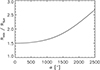 |
Fig. 7 Height of the closest point of the ray path to the Sun, as a function of viewing angle α, for Rω = 1.5 R⊙, a scale height temperature T = 1.4× 10⁶ K, and observing frequency f = 54 MHz. |
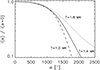 |
Fig. 8 Intensity profiles from three ray-tracing simulations with Rω = 1.5 R⊙ and differentscale height temperatures: T = 1.4 × 10⁶ K (solid line), T = 1.0 × 10⁶ K (dashed line), and T = 1.8 × 10⁶ K (dotted line), all for an observing frequency f = 54 MHz. |
3.3 Coronal density model based on LOFAR images
Before an observed intensity profile can be fitted with ray-tracing simulations with variable values of Rω and T, the finite angular resolution of radio observations has to be considered. To take this into account, the model intensity profiles are convolved with a Gaussian beam profile. For the observations presented in this work, a FWHM beam of 150″ is typical. However, this has little effect on the simulated profiles.
Figure 9 shows the result of such a fit to the observed 54 MHz polar intensity profile. As stated above, the polar regions of the Sun show a simple, radial magnetic field geometry that matches well the ray-tracing simulations with their local hydrostatic density model in the radial direction. The simulation parameters that provide the best fit are Rω = 1.36 R⊙, and a scale height temperature of T= 1.85 × 10⁶ K. This is a surprisingly high value, much more than the usual T = 1.0−1.4 × 10⁶ K in coronal density models such as those of Mann et al. (1999) or Newkirk (1961).
But thishigh temperature does provide the best fit; the model intensity profile is in close agreement with the observed profile for α <1600″. A variation of T mainly leads to different slopes of the simulated profile for larger α > 1000″ (see Fig. 8). So a lower temperature value would lead to a steeper intensity profile, not in agreement with the observed profile. For larger α > 1600″, the slope of the observed intensity profile starts to be steeper than the model profile, as if a lower temperature value was relevant there.
The scale height temperature value T has its strongest impact on the outer, high α part of simulated intensity profiles. This enables a quick test of the method of line-of-sight integration over emissivities and absorption, which is based on Eqs. (1)–(3). If the emission and absorption terms are replaced by a simple line integral over  , i.e., all effects of finite optical depth are ignored, then it is found that this manipulation has little effect on the slope of the outer part of the profile. The reason for this behavior is that for higher α, the ray path only traverses higher, and therefore more dilute regions, of the corona, where the optical depth is low. But still, the same high coronaltemperature is needed to fit the observation. This test indicates that the high temperature is a robust result, and not an artifact based on a flaw of the ray-tracing simulations using Eqs. (1)–(3).
In order to study the dependence of the fit quality on the model parameters Rω and T, and to estimate error margins for these, wedefine residuals χ2 as a measure for the difference between model and observed intensity profiles in a semi-logarithmic plot, that is,
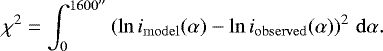 (7)
(7)
Minimizing χ2 corresponds to a least-square fit to the observed profile. The upper boundary of the integral was chosen as α = 1600″, where both profiles start deviating from each other.
Figure 10 shows the residuals χ as functions of Rω and T. Low values of χ2 form a line in Rω − T space, with a minimum at Rω = 1.36 R⊙ and T = 1.85 × 10⁶K, which provide the best fit and minimize χ2. The width of the area with lowest χ2 provides estimates for error margins of ± 0.01 R⊙ for Rω and ± 5 × 10⁴ K for T. Significantly lower temperatures, for example,T = 1.4 × 10⁶ K, increase the residuals χ2 by more than one order of magnitude.
The same fitting procedure is now repeated for all other observed frequencies. Figure 11 shows the frequencies, f, as a function of the fitted values for Rω. Since Rω is where the local plasma frequency equals the observation frequency, this plot corresponds to a density profile, Ne (r). The solid line represents a hydrostatic coronal density model based on a constant coronal temperature of T =2.2 × 10⁶ K and a density N0 = 1.6 × 10¹⁴ m−3 at the coronal base. The dotted line delineates a density profile that scales as Ne (r) ∝ 1∕r2, which is discussed below.
Figure 12 shows the corresponding coronal temperatures. It is obvious that the T =1.9 × 10⁶ K found for f = 54 MHz is not even the highest value. In the low corona, i.e., for the highest frequencies, T reaches up to 2.2 × 10⁶ K. We note that these temperature values were obtained for each observed frequency independently.
The temperature T = 2.2 × 10⁶ K that was used in the hydrostatic model fit of the density values in the low corona (see Fig. 11) provides the best fit to the data. A lower temperature leads to a density decrease with height that is too fast. This result is independent of the fitting procedure for individual intensity profiles as in Fig. 9. So the high scale height temperature in the low corona is a consistent result that has been obtained from two independent methods.
The coronal temperature profile in Fig. 12 also provides an explanation for the deviation of the fit in Fig. 9 for higher viewing angles α > 1600″. With increasing α, the ray path traverses higher layers of the corona, where the temperature is indeed lower, as already indicated in the discussion of the fit in Fig. 9. The poor fit for higher α is therefore an artifact of the model assumption of a constant scale height temperature. For smaller α, this is not critical, since the minimum distance of the ray path to the Sun depends less on α (see Fig. 7).
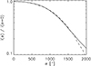 |
Fig. 9 Model (solid line) and observed (dashed line) intensity profiles for an observing frequency f = 54 MHz. The simulation parameters are Rω = 1.36 R⊙ and T = 1.85 × 10⁶K. |
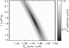 |
Fig. 10 Residuals χ2 between model and observed intensity profiles, as functions of fitting parameters Rω and T. |
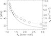 |
Fig. 11 Observed frequencies, f, as a functionof fitted Rω, together with a hydrostatic density model (solid line) and 1∕r2 density model (dotted line). |
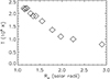 |
Fig. 12 Fitted scale height temperature values, as a function of the Rω, fitted to each observed frequency. |
4 Discussion
It has been shown that LOFAR images of the quiet solar corona allow for the derivation of coronal density and temperature values. This is performed individually for each observed frequency by fitting a model intensity profile across the radio Sun, based on a ray-tracing simulation, to the observed profile. The density is obtained in the form of the radius Rω, where the local plasma frequency equals the observed frequency, ω. In this paper, we only studied intensity profiles in the polar direction, with their simpler, radial magnetic field geometry.
The results show surprisingly high scale height temperatures of 2.2 × 10⁶ K in the low corona. This temperature describes the density decrease with altitude, that is directly observed in coronal white-light scattering. Density models based on such observations lead to much lower temperatures of T = 1.4 × 10⁶ K, such as those of Newkirk (1961). Other coronal models, such as that of Mann et al. (1999), who fits a Parker-type solar coronal and wind model to observations ranging from the corona up to 1 AU, also indicate temperatures closer to T = 106 K.
But if the Rω and temperatures from all observed frequencies are combined, they lead to a coherent picture. The temperature profile (see Fig. 12) shows a continuous decrease from the 2.2 × 10⁶ K in the low corona to less than 106 K in the outer corona. The Rω values can be combined into a density profile, which can be fitted by a hydrostatic model for small heights below 1.4 R⊙. But the hydrostatic model has to be based on the same high temperature of T = 2.2 × 10⁶ K. It should be noted that the scale height temperature in such a single-fluid model is a combination of electron and ion temperatures.
This agreement is an indication that the temperature results are correct, since the fits to the intensity profiles were carried out for each frequency, i.e., coronal height, independently. The density model that results from all values for Rω combined together, thus is consistent with such a high temperature. The reason for this is unclear, since the SDO images indicate no signs of activity in the polar regions.
The hydrostatic model is based on a density at the coronal base of N0 = 1.6 × 10¹⁴ m−3. This is very low for the quiet Sun, it corresponds to just one-fifth of the value in the model of Newkirk (1961). It would be more typical for acoronal hole, although a coronal hole is not visible in the SDO images.
The high temperatures of up to T = 2.2 × 10⁶ K have been found at low radial distances of less than 1.5 R⊙. This altitude range has been studied by Mercier & Chambe (2015), at higher frequencies with the NRH. They have also found relatively high scale height temperatures in the north–south direction in their Fig. 6, varying between 1.65× 10⁶ K and 2.24× 10⁶ K. So there is some consistency with these observations.
Extreme UV observations are another source for coronal temperature data, i.e., coronal electron temperatures, Te. However, it is a long-standing issue that the observed Te on the orderof 106 K are higher than brightness temperatures at the solar disk center of about 7 × 10⁵ K (Dulk et al. 1977). Reconciling these temperatures requires further model assumptions (Chiuderi Drago et al. 1999). The scale height temperatures, T, discussed here is not Te, but results as an average of both electron and ion temperatures. Even a Te = 106 K would require an average ion temperatureof about Ti = 3.4 × 10⁶ K for a scale height temperature of 2.2 × 10⁶ K. Minor ions, such asO5+, are observed to have very high temperatures up to 108 K (Antonucci et al. 2012), but these values are found higher up in the corona above 2 R⊙ and not for the bulk of protons. Below 2 R⊙, O5+ temperatures drop to 8 × 10⁶ K at 1.4 R⊙, so minor ions with their relative abundances well below 10−3 (Grevesse & Sauval 1998) should not have a significant influence on lower coronal scale heights. The issue of high scale height temperatures in the low corona in the radio data has to be left open for future research.
For larger coronal heights, around 1.5 R⊙, the Rω become larger than predicted by the hydrostatic model. In other words, the density falls off slower than hydrostatically. The temperature is already lower in this region, which should lead to an even faster density decrease than predicted by the T = 2.2 × 10⁶ K hydrostatic model.
This is the expected behavior for the transition from the subsonic plasma flow in the corona into the supersonic solar wind, where the density falls off as r−2 once a constant solar wind speed has been reached. A significant deviation from a hydrostatic profile is to be expected once the sonic Mach number, M, does not satisfy the condition M ≪ 1 anymore. The dotted line in Fig. 11 shows such an Ne(r) ∝ 1∕r2 profile. This profile fits the data well in the upper corona, even as low as 1.5 R⊙.
This indicates a transition into the supersonic solar wind that is located rather low in the corona, but still in agreement with some solar wind models (Axford et al. 1999). Furthermore, similar nonhydrostatic density profiles have also been found in the analysis of type III radio bursts (Cairns et al. 2009).
The ray tracing simulations, based on Eqs. (1) and (3) used to calculate model intensity profiles, which are then fitted to the observed profiles as in Fig. 9, stem from an important assumption. The profiles are calculated as if the coronal density decreases hydrostatically above Rω. But in the transition to the solar wind, the corona is not hydrostatic anymore. However, this hydrostatic assumption is not used to calculate a density model of the whole corona. Instead, it only describes the density decrease just above Rω. At larger heights, the free-free radiation emissivity decreases with the square of the density, such that there is only a minor contribution to the line-of-sight integrals the model intensity profiles are based on.
To the first order, the density decrease above Rω can be described by the hydrostatic model, Eq. (6), even if the corona is not hydrostatic. The derivative of Eq. (6) in r at the position r = Rω can be written as
 (8)
(8)
Replacing the left-hand side of Eq. (8) by the logarithmic coronal density gradient, which has been derived from the data, then allows for calculating H0, and through Eq. (5) the scale height temperature T. For a nonhydrostatic corona, this is not the actual temperature, but just a parameter describing the density decrease with height. If the coronal density, for example, falls off slower than hydrostatically, this T would be higher than the temperature there.
For the temperature values shown in Fig. 12, this has the consequence that those from coronal heights above 1.5 R⊙ should be treated with caution. But in the low corona, where the high T = 2.2 × 10⁶ K have been found, a hydrostatic density model seems to be applicable. So the hydrostatic model assumption in the ray-tracing simulations seems unlikely to be responsible for the high temperatures found there.
5 Summary and outlook
The analysis of these first quiet-Sun Earth-rotation interferometric imaging observations with LOFAR show their potential for investigating the coronal structure. Density models can be derived and the transition from the hydrostatic lower solar corona into the supersonic solar wind can be studied.
But the interpretation of coronal radio images is not straightforward. The effects of the refractive medium of the solar corona on radio wave propagation, including free–free wave emission and absorption, need to be taken into account. Considering these effects, it is possible to calculate intensity profiles across the Sun with ray-tracing simulations.
For the first results presented here, we focused on the simple, radial magnetic-field geometry above the poles of the quiet Sun. More complex structures such as closed loops were not studied.
The Sun was only observed on a few selected frequencies, with 5 MHz gaps between them, for these early LOFAR data. Future observations provide a continuous frequency coverage in LOFAR’s low band of 10–90 MHz, with a frequency resolution that corresponds to the LOFAR 195 kHz sub-band width.
With continuous frequency coverage, it will be possible to derive iteratively a single coronal density model that can be used for all ray-tracing simulations for different frequencies. This eliminates the need for a local hydrostatic density model in the data analysis, and thereby the need to fit model intensity profiles not only to Rω, but also to a scale height temperature value. An example would be studies of equatorial density profiles that could traverse closed magnetic field lines connecting active regions such as those in the SDO image (Fig. 2). For such structures, the model simplification of local hydrostatic equilibrium is at least questionable. This is why we did not perform the analysis in the present paper.
Scale height temperatures still can be derived from the barometric scale height of the density profile as long as the corona can be considered in hydrostatic equilibrium. This will provide a test of whether the high temperatures of more than 2 × 10⁶ K will still be found.
Such animproved method will lead to a better analysis of data for the upper corona, where the transition into the supersonic solar wind occurs and where a local hydrostatic model is a rough approximation. Furthermore, it will enable studies of more complex coronal structures, where a local hydrostatic density model is not applicable at all. Thus not only the quiet Sun and coronal holes, but also closed loops and streamer-like structures will be investigated.
Acknowledgements
C. Vocks, G. Mann, and F. Breitling acknowledge the financial support by the German Federal Ministry of Education and Research (BMBF) within the framework of the project D-LOFAR (05A11BAA) of the Verbundforschung. This paper is based on data obtained with the International LOFAR Telescope (ILT). LOFAR (van Haarlem et al. 2013) is the Low Frequency Array designed and constructed by ASTRON. It has facilities in several countries, which are owned by various parties (each with their own funding sources) and which are collectively operated by the ILT foundation under a joint scientific policy. The authorswish to thank the referee for constructive comments that have helped to improve the manuscript significantly.
References
- Alissandrakis, C. E. 1994, Adv. Space Res., 14 [Google Scholar]
- Antonucci, E., Abbo, L., & Telloni, D. 2012, Space Sci. Rev., 172, 5 [NASA ADS] [CrossRef] [Google Scholar]
- Axford, W. I., McKenzie, J. F., Sukhorukova, G. V., et al. 1999, Space Sci. Rev., 87, 25 [NASA ADS] [CrossRef] [Google Scholar]
- Breitling, F., Mann, G., Vocks, C., Steinmetz, M., & Strassmeier, K. G. 2015, Astron. Comput., 13, 99 [NASA ADS] [CrossRef] [Google Scholar]
- Cairns, I. H., Lobzin, V. V., Warmuth, A., et al. 2009, ApJ, 706, L265 [NASA ADS] [CrossRef] [Google Scholar]
- Chiuderi Drago, F., Landi, E., Fludra, A., & Kerdraon, A. 1999, A&A, 348, 261 [Google Scholar]
- Dulk, G. A., Sheridan, K. V., Smerd, S. F., & Withbroe, G. L. 1977, Sol. Phys., 52, 349 [NASA ADS] [CrossRef] [Google Scholar]
- Grevesse, N., & Sauval, A. J. 1998, Space Sci. Rev., 85, 161 [NASA ADS] [CrossRef] [Google Scholar]
- Kerdraon, A., & Delouis, J.-M. 1997, in Coronal Physics from Radio and Space Observations, ed. G. Trottet, Lect. Notes Phys. (Berlin: Springer Verlag), 483, 192 [NASA ADS] [CrossRef] [Google Scholar]
- Kundu, M. R., Gergely, T. E., Turner, P. J., & Howard, R. A. 1983, ApJ, 269, L67 [NASA ADS] [CrossRef] [Google Scholar]
- Kundu, M. R., Gergely, T. E., Schmahl, E. J., Szabo, A., & Loiacono, R. 1987, Sol. Phys., 108, 113 [NASA ADS] [CrossRef] [Google Scholar]
- Lantos, P. 1999, in Proc. of the Nobeyama Symposium, eds. T. S. Bastian, N. Gopalswamy, & K. Shibasaki, 479, 11 [NASA ADS] [Google Scholar]
- Mann, G. 2010, in Instruments and Methods, Landolt-Börnstein (Berlin Heidelberg: Springer-Verlag), 216 [Google Scholar]
- Mann, G., Jansen, F., MacDowall, R. J., Kaiser, M. L., & Stone, R. G. 1999, A&A, 348, 614 [NASA ADS] [Google Scholar]
- Mann, G., Vocks, C., & Breitling, F. 2011, Solar Observations with LOFAR, 7th International Workshop on Planetary, Solar and Heliospheric Radio Emissions (PRE VII) (Graz, Austria), eds. H. O. Rucker, W. S. Kurth, P. Louarn, & G. Fischer, 507 [Google Scholar]
- McLean, D. J., & Melrose, D. B. 1985, Propagation of Radio Waves Through the Solar Corona, ed. [Google Scholar]
- Mercier, C., & Chambe, G. 2015, A&A, 583, A101 [NASA ADS] [CrossRef] [EDP Sciences] [Google Scholar]
- Mercier, C., Subramanian, P., Chambe, G., & Janardhan, P. 2015, A&A, 576, A136 [NASA ADS] [CrossRef] [EDP Sciences] [Google Scholar]
- Morosan, D. E., Gallagher, P. T., Zucca, P., et al. 2014, A&A, 568, A67 [NASA ADS] [CrossRef] [EDP Sciences] [Google Scholar]
- Newkirk, Jr., G. 1961, ApJ, 133, 983 [NASA ADS] [CrossRef] [Google Scholar]
- Priest, E. R. 1982, in Solar Magneto-Hydrodynamics (Dordrecht, Holland, Boston, Hingham: D. Reidel Pub. Co.), 82 [Google Scholar]
- Ramesh, R., Subramanian, K. R., Sundararajan, M. S., & Sastry, C. V. 1998, Sol. Phys., 181, 439 [Google Scholar]
- Ramesh, R., Kathiravan, C., & Sastry, C. V. 2010, ApJ, 711, 1029 [NASA ADS] [CrossRef] [Google Scholar]
- Shibasaki, K., Alissandrakis, C. E., & Pohjolainen, S. 2011, Sol. Phys., 273, 309 [Google Scholar]
- Smerd, S. F. 1950, Aust. J. Sci. Res. A Phys. Sci., 3, 34 [NASA ADS] [Google Scholar]
- van Haarlem, M. P., Wise, M. W., Gunst, A. W., et al. 2013, A&A, 556, A2 [NASA ADS] [CrossRef] [EDP Sciences] [Google Scholar]
- Wang, Z., Schmahl, E. J., & Kundu, M. R. 1987, Sol. Phys., 111, 419 [NASA ADS] [CrossRef] [Google Scholar]
- Wild, J. P. 1970, Proc. Astron. Soc. Aust., 1, 365 [NASA ADS] [CrossRef] [Google Scholar]
All Figures
|
Fig. 1 uv coverage of the solar observations for snapshot imaging (left) and an observing time of 3 h (right). |
| In the text | |
|
Fig. 2 Nançay Radioheliograph image at 150.9 MHz (left), and EUV image from the Solar Dynamics Observatory (SDO) in the Fe IXline at 171 Å (right). |
| In the text | |
|
Fig. 3 Images of the Sun from LOFAR from 8 August 2013, 08:02–11:02 UT, for several low-band frequencies ranging from 25 to 79 MHz. |
| In the text | |
|
Fig. 4 Brightness temperature profiles derived from the 74 MHz image for polar (solid line) and equatorial (dashed line) regions. |
| In the text | |
|
Fig. 5 Geometry of radio wave refraction in the solar corona. |
| In the text | |
|
Fig. 6 Intensity profiles from two ray-tracing simulations with Rω = 1.7 R⊙ (solid line) and Rω = 1.5 R⊙ (dashed line), both for a coronal scale height temperature of T = 1.4 × 10⁶ K and an observing frequency f = 54 MHz. |
| In the text | |
|
Fig. 7 Height of the closest point of the ray path to the Sun, as a function of viewing angle α, for Rω = 1.5 R⊙, a scale height temperature T = 1.4× 10⁶ K, and observing frequency f = 54 MHz. |
| In the text | |
|
Fig. 8 Intensity profiles from three ray-tracing simulations with Rω = 1.5 R⊙ and differentscale height temperatures: T = 1.4 × 10⁶ K (solid line), T = 1.0 × 10⁶ K (dashed line), and T = 1.8 × 10⁶ K (dotted line), all for an observing frequency f = 54 MHz. |
| In the text | |
|
Fig. 9 Model (solid line) and observed (dashed line) intensity profiles for an observing frequency f = 54 MHz. The simulation parameters are Rω = 1.36 R⊙ and T = 1.85 × 10⁶K. |
| In the text | |
|
Fig. 10 Residuals χ2 between model and observed intensity profiles, as functions of fitting parameters Rω and T. |
| In the text | |
|
Fig. 11 Observed frequencies, f, as a functionof fitted Rω, together with a hydrostatic density model (solid line) and 1∕r2 density model (dotted line). |
| In the text | |
|
Fig. 12 Fitted scale height temperature values, as a function of the Rω, fitted to each observed frequency. |
| In the text | |
Current usage metrics show cumulative count of Article Views (full-text article views including HTML views, PDF and ePub downloads, according to the available data) and Abstracts Views on Vision4Press platform.
Data correspond to usage on the plateform after 2015. The current usage metrics is available 48-96 hours after online publication and is updated daily on week days.
Initial download of the metrics may take a while.