| Issue |
A&A
Volume 613, May 2018
|
|
|---|---|---|
| Article Number | L1 | |
| Number of page(s) | 5 | |
| Section | Letters to the Editor | |
| DOI | https://doi.org/10.1051/0004-6361/201832664 | |
| Published online | 18 May 2018 | |
Letter to the Editor
The evolution of the X-ray afterglow emission of GW 170817/ GRB 170817A in XMM-Newton observations
1
INAF – Osservatorio Astronomico di Brera,
Via E. Bianchi 46,
23807
Merate (LC), Italy
e-mail: paolo.davanzo@brera.inaf.it
2
Dipartimento di Fisica “G. Occhialini”, Università degli Studi di Milano-Bicocca,
Piazza della Scienza 3,
20126
Milano, Italy
3
INFN – Sezione di Milano-Bicocca,
Piazza della Scienza 3,
20126
Milano, Italy
4
Gran Sasso Science Institute,
Viale F. Crispi 7,
L’Aquila, Italy
5
Laboratoire Univers et Particules de Montpellier, Université Montpellier, CNRS/IN2P3,
Montpellier, France
6
INFN, Laboratori Nazionali del Gran Sasso,
67100
L’Aquila, Italy
7
APC, Université Paris Diderot, CNRS/IN2P3, CEA/Irfu, Obs de Paris,
Sorbonne Paris Cité, Paris, France
8
Space Science Data Center, ASI, Via del Politecnico, s.n.c.,
00133
Roma, Italy
9
INAF, Osservatorio Astronomico di Trieste,
Via G.B. Tiepolo 11,
34143
Trieste, Italy
10
INAF, Istituto di Astrofisica Spaziale e Fisica Cosmica di Milano,
via E. Bassini 15,
20133
Milano, Italy
11
GEPI, Observatoire de Paris, PSL Research University, CNRS, Place Jules Janssen,
92190
Meudon, France
Received:
18
January
2018
Accepted:
17
April
2018
We report our observation of the short gamma-ray burst (GRB) GRB 170817A, associated to the binary neutron star merger gravitational wave (GW) event GW 170817, performed in the X-ray band with XMM-Newton 135 d after the event (on 29 December, 2017). We find evidence for a flattening of the X-ray light curve with respect to the previously observed brightening. This is also supported by a nearly simultaneous optical Hubble Space Telescope observation and successive X-ray Chandra and low-frequency radio observations recently reported in the literature. Since the optical-to-X-ray spectral slope did not change with respect to previous observations, we exclude that the change in the temporal evolution of the light curve is due to the passage of the cooling frequency: its origin must be geometric or dynamical. We interpret all the existing afterglow data with two models: i) a structured jet and ii) a jet-less isotropic fireball with some stratification in its radial velocity structure. Both models fit the data and predict that the radio flux must decrease simultaneously with the optical and X-ray emission, making it difficult to distinguish between them at the present stage. Polarimetric measurements and the rate of short GRB-GW associations in future LIGO/Virgo runs will be key to disentangle these two geometrically different scenarios.
Key words: gravitational waves / gamma rays: general
© ESO 2018
1 Introduction
A gravitational wave (GW) event originated by the merger of a binary neutron star (BNS) system was detected for the first time by aLIGO/Virgo (GW 170817; Abbott et al. 2017a), and was found to be associated to the weak short gamma-ray burst (GRB) GRB 170817A detected by the Fermi and INTEGRAL satellites (Goldstein et al. 2017; Savchenko et al. 2017), marking the dawn of multi-messenger astronomy (Abbott et al. 2017b). The proximity of the event ~41 Mpc; Hjorth et al. 2017, Cantiello et al. 2018) and the relative accuracy of the localisation (~30 deg2, thanks to the joint LIGO and Virgo operation) led to a rapid (Δt < 11 h) identification of a relatively bright optical electromagnetic counterpart (EM), named AT2017gfo, in the galaxy NGC 4993 (Arcavi et al. 2017; Coulter et al. 2017; Lipunov et al. 2017; Melandri et al. 2017; Tanvir et al. 2017; Soares-Santos et al. 2017; Valenti et al. 2017). The analysis and modelling of the spectral characteristics of this source, together with their evolution with time, resulted in a good match with the expectations for a “kilonova” (i.e. the emission due to radioactive decay of heavy nuclei produced through rapid neutron capture; Li & Paczyński 1998), providing the first compelling observational evidence for the existence of such elusive transient sources (Cowperthwaite et al. 2017; Drout et al. 2017; Evans et al. 2017; Kasliwal et al. 2017; Nicholl et al. 2017; Pian et al. 2017; Smartt et al. 2017; Villar et al. 2017). While the bright kilonova associated to GW 170817 has been widely studied and its main properties relatively well determined, the observations of the short GRB 170817A are more challenging for the current theoretical frameworks. Indeed, the properties of this short GRB appear puzzling in the context of observations collected over the past decades (Berger 2014; D’Avanzo 2015; Ghirlanda et al. 2015). The prompt γ-ray luminosity was significantly fainter (by a factor ~2500) than typical short bursts (see, e.g. D’Avanzo et al. 2014). A faint afterglow was detected in the X-ray and radio bands only at relatively late times (starting from ~9 and 16 d after the GW/GRB trigger, respectively; Alexander et al. 2017; Haggard et al. 2017; Hallinan et al. 2017; Margutti et al. 2017; Troja et al. 2017a), while earlier observations provided only upper limits in these bands (Evans et al. 2017; Hallinan et al. 2017).
Similarly to long bursts, short GRBs are thought to be produced by a relativistic jet with a typical half-opening angle θjet ~ 5–15 deg (Fong et al. 2016). However, whether or not BNS mergers can always efficiently produce a relativistic jet is still debated (Paschalidis et al. 2015; Ruiz et al. 2016; Kawamura et al. 2016). Given the small probability that our line of sight was within the jet half-opening angle, 1 − cos(θjet), it is unlikelythat the first short GRB associated to a GW event had a jet pointing towards the Earth. The extremely low γ-ray luminosity of GRB 170817A has been interpreted as being due to (i) the debeamed radiation of a jet observed off-beam (i.e. viewing angle θview > θjet), provided that the jet bulk Lorentz factor is significantly smaller than usually assumed (see, e.g. Pian et al. 2017). Alternatively, the jet could be (ii) structured, with a fast and energetic inner core surrounded by a slower, less energetic layer/sheath/cocoon (first proposed for long GRBs – Lipunov et al. 2001; Rossi et al. 2002; Salafia et al. 2015 – and only recently extended to short GRBs – Kathirgamaraju et al. 2018; Lazzati et al. 2017a; Gottlieb et al. 2017; Lazzati et al. 2017b; Lyman et al. 2018; Margutti et al. 2018; Troja et al. 2018a). In this scenario the faint, off-beam emission is due to the slower component, which originates from the interaction of the jet with the merger dynamical ejecta or the post-merger winds. Recently, Mooley et al. (2018) suggested the possibility that (iii) the jet was not successful in excavating its way through the ambient medium and that GRB 170817A was due to its vestige, a quasi-isotropic cocoon with a velocity profile. Last but not least, (iv) a jet-less interpretation of GRB 17017A could still be viable: an isotropic fireball, expanding ahead of the kilonova ejecta, which could account for both the low luminosity of the γ-ray event and the properties of the EM component in the radio and X-ray bands (Salafia et al. 2017). In this case, all BNS mergers should have this kind of faint, hard X-ray counterpart. All of the above scenarios have relatively clear predictions for the temporal and spectral evolution of the electromagnetic emission from X-rays to the radioband. A comprehensive discussion of the possible physical scenarios leading to the observed broad-band emission of GW 170817/GRB 170817A can be found in Nakar & Piran (2018). Recent radio and X-ray observations(Mooley et al. 2018; Margutti et al. 2018; Ruan et al. 2018; Troja et al. 2018a), carried out until ~ 110−115 d after the event, indicate that the source flux is steadily rising and that the spectral energy distribution (SED) over these bands is consistent with a single power-law component. These results disfavour interpretation (i) reported above (an off-beam homogeneous jet).
In this Letter we present deep, late-time X-ray observations of GW 170817/GRB 170817A carried out ~135 days after the event with the XMM-Newton satellite, showing evidence for a a change in the temporal slope, indicating a flattening in the afterglow emission (Sect. 2). In Sect. 3 we interpret and discuss all the available afterglow data of GW 170817 / GRB 170817A under the structured jet and jet-less scenarios mentioned above and summarise our conclusions in Sect. 4.
2 Observations and data analysis
XMM-Newton started observing GW 170817 on 29 December 2017 at 19:00:11 UT, 134.5 d after the GW event. XMM-Newton observed for 41.3 ks (42.8 ks) with the pn (MOS) detector, all equipped with the thin filter. Two large background flares occurred during the observation, reducing the usable time to 26.0 and 29.6 ks for the pn and MOS detectors, respectively. The centre of NGC 4993 lies at only 10″ from GW 170817 (see Fig. 1) and particular care must be taken. We extracted products using a region of 4″ radius centred on the optical position of GW 170817/GRB 170817A (Coulter et al. 2017). The background has been extracted from two 4″ regions, at the same distance from the host galaxy centre, one opposite to GW 170817 and the other to the north-east (thus avoiding the source detected by Chandra, named “S2” in Margutti et al. (2018), in the south-west region). We gathered (source plus background) 60, 15 and 15 counts from the pn, MOS1 and MOS2 detectors, respectively, with the source making 70− 80% of the total. Response matrices were generated with the package SAS v16.1 using the latest calibration products.
Spectra were rebinned to five counts per spectral bin and C-statistics was adopted for the fits. We fit the three spectra with an absorbed power law model with the column density fixed to a Galactic value of 7.84 × 1020 cm−2 (Kalberla et al. 2005). A 90% confidence level (c.l.) upper limit on the intrinsic absorption is <1.1 × 1021 cm−2. The best fit provides a photon index  (90% c.l.) and a 0.3–10 keV unabsorbed flux
 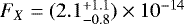 erg cm−2 s−1. This fit and its uncertainty region are shown in Fig. 2 by the dot–dashed line and the grey shaded region, respectively. The XMM-Newton de-absorbed data are also shown in Fig. 2 (blue points).
Motivated by the almost simultaneous XMM-Newton and HST observations (~137 d after the event; Margutti et al. 2018), we dereddened1 the optical AB magnitude magF606W = 26.90 ± 0.25 reported by these authors and we fitted together optical and X-ray data. Thanks to the large leverage in terms of energy range, we tightly constrain the overall power law photon index to Γ = 1.60 ± 0.05. This fit is shown by the dashed red line and its uncertainty by the yellow shaded region in Fig. 2. Adopting this index in the range 0.3–10 keV, the unabsorbed flux is 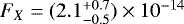 erg cm−2 s−1, which translates to a luminosity LX = 4 × 1039 erg s−1 (at 41 Mpc). The XMM-Newton flux and photon index are fully consistent with the values found about one month before and after our observation by Chandra (namely, a 0.3–10 keV unabsorbed flux FX = (2.5 ± 0.3) × 10−14 erg cm−2 s−1 and FX = (2.6 ± 0.3) × 10−14 erg cm−2 s−1 measured at ~ 109 and 159 days after the GW trigger, respectively; Margutti et al. 2018; Troja et al. 2018a,b) and indicate that the GW 170817 flux stopped increasing.
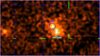 |
Fig. 1 X-ray image obtained by co-adding the XMM-Newton pn and MOS data presented in this paper. The X-ray emission of GW 170817/GRB 170817A (upper circle, 4″ radius) is clearly visible close to the nucleus of its host galaxy NGC 4993 (lower circle). |
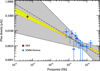 |
Fig. 2 Optical to X-ray spectrum of GRB 170817A. XMM-Newton data points (blue, this work) and HST contemporaneous detection (red circle) are shown. The grey shaded region shows the 90% uncertainty on the fit of the XMM-Newton data alone (dot-dashed line). The fit obtained combining the de-reddened HST flux (from Margutti et al. 2018) and our XMM-Newton data results in a photon index of 1.6 (dotted red line) with an error of ± 0.05 (90% c.l. – yellow shaded region). |
3 Interpretation and discussion
Figure 3 shows the afterglow data published in the literature to date, together with our XMM-Newton point obtained at ~ 135 d (light blue circle). All radio and X-ray detections of GRB 170817A reported so far covering the time range between ~9 and ~115 d after the event indicated a steady increase of the source flux (F(t) ∝ t0.7−0.8), with negligible spectral evolution over a broadband spectrum (Fν ∝ ν−0.6; Mooley et al. 2018; Margutti et al. 2018; Ruan et al. 2018; Troja et al. 2018a). By comparing the nearly simultaneous XMM-Newton and HST observations (see Sect. 2) we find that the SED at the epoch of our XMM-Newton observation is still consistent with a single power–law component between the X-ray and the optical, with Fν ∝ν−0.6 (Fig. 2). Given the lack of spectral evolution, we found it reasonable to assume that the light curve is evolving in the same way at all wavelengths and carried out a combined fit of the available radio (3 GHz), optical2 and X-ray (0.3–10 keV) data obtained between ~9 and ~159 d after the event (Hallinan et al. 2017; Mooley et al. 2018; Lyman et al. 2018; Margutti et al. 2018; Troja et al. 2018a,b). Using an F-test we compared the joined fit obtained with a single and a broken power-law model. We find that a temporal break is required at 1.94σ (95% c.l.). While with a single power-law (F(t) ∝ tα) model we obtain an index α ~ 0.8, in agreement with other findings (Mooley et al. 2018; Margutti et al. 2018; Troja et al. 2018a), at the same time we note that both the XMM-Newton (this work) and Chandra3 (Troja et al. 2018b) data points obtained at successive epochs over two months fall below the extrapolation of the best fit (by 1.5 and 2.7 sigma, respectively). Such an increasing divergence, together with the mild indication of a temporal break provided by the F-test, is indicative of a change in the slope, with a flattening, of the X-ray light curve with respectto the brightening trend observed in the X-ray and radio bands at earlier epochs. This change in the light curve temporal evolution is observed also in the optical band by the HST observations carried out at ~ 110 and ~ 137 d with HST (Lyman et al. 2018; Margutti et al. 2018; see also Fig. 3). Furthermore, the evidence for a possible plateau in the light curve has recently been found in low-frequency radio data obtained between 66 and 152 days after the event (Resmi et al. 2018), although the relatively poor temporal sampling prevents us from firmly excluding a rising trend. Overall, the multi-wavelength behaviour of the afterglow provides an indication that the light curve is changing slope (see also Dobie et al. 2018), even if it is too early to constrain the temporal evolution after the break, since at this epoch we are still sampling its turning point.
The X-ray spectrum expected if the cooling frequency has transitioned below the X-ray band (between the earlier Chandra observation and our XMM-Newton epoch) has a photon index of 2.1 and predicts an optical flux that is inconsistent with that observed by HST at almost the same epoch. We can therefore exclude this explanation of the observed optical and X-ray light curve peak. We rather interpret it as being due to a dynamical or geometric effect. We interpret the optical and X-ray light curve within two possible scenarios: (i) a structured jet, in which case the decline of the optical and X-ray fluxes indicates that the emission from the jet core has entered our line of sight (i.e. the core has decelerated down to a Lorentz factor  ); or (ii) an isotropic (Salafia et al. 2017) and stratified fireball with a velocity profile, like that described in Mooley et al. (2018), in which case the light curve peak indicates that the velocity profile has a rather sharp cut-off at βmin = vmin∕c ~ 0.88.
3.1 The structured jet model
If a jet is launched after the merger, it must excavate its way out of the inner region, which can be baryon-polluted due to the post-merger winds and the dynamical ejecta. The propagation through such ambient material is likely to play a major role in shaping the jet angular distribution of energy and terminal Lorentz factor at breakout (see e.g. the simulations by Lazzati et al. 2017b). The resulting jet structure features an inner, narrow, faster core with a relatively uniform distribution of kinetic energy per unit solid angle, surrounded by a slower, extended structure whose kinetic energy per unit solid angle decreases relatively quickly with the distance from the jet axis. This latter structure can be identified as the vestige of the jet cocoon (constituted by the jet and ambient material that has been shocked during the excavation). Guided by this picture, we employ a simple structured jet model, in which both the isotropic equivalent kinetic energy EK,iso and the bulk Lorentz factor Γ are approximately constant within a narrow core of half-opening angle θcore and decrease as power-laws outside of it:
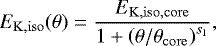 (1)
and
(1)
and
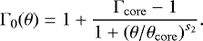 (2)
(2)
We model the dynamics of the jet with the simplifying assumption that each solid angle element evolves independently (i.e. we neglect side expansion, which should have a limited effect on the light curve, see e.g. Granot & Kumar 2003; Lazzati et al. 2017b; Lamb & Kobayashi 2017). For each solid angle element, we model the emission following Sari et al. (1998), with the proper transformations to the off-axis observer frame. The ambient medium is assumed to have a constant number density n. The parameters of the structured jet model shown in Fig. 3 (dashed lines) are reported in Table 1 (where ϵe and ϵB are the shock energy carried by the electrons and by the magnetic field, respectively, and p is the electron energy distribution index). With the given parameters, the total kinetic energy in the jet is Ejet ≈ 1.1 × 1049 erg (for one jet), which is just what is expected for a standard short GRB jet (Hotokezaka et al. 2016). Different structured jet scenarios have been proposed to model the afterglow light curves of GRB 170817A by Lazzati et al. (2017b), Lyman et al. (2018), Margutti et al. (2018) and Troja et al. (2018a). As in our case described above, the models presented in Lyman et al. (2018), Margutti et al. (2018) and Troja et al. (2018a) can account for the change in the slope observed in the X-ray and optical light curve at t ~ 110−130 d, predicting a relatively long plateau at these epochs. We note, however, that all the proposed models are very similar and that the diversity in the predictions can be ascribed to a combination of differences in the jet structure (including the opening angle of the relativistic core) and the density of the environment, and to the different choice of the microphysical parameters, that can be better constrained with future multi-band observations.
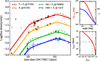 |
Fig. 3 Left-hand panel: GRB 170817A afterglow light curves in radio at 3 GHz and 6 GHz (red and orange stars, respectively, VLA observations – data from Hallinan et al. 2017; Mooley et al. 2018), in the optical (green stars, HST/ACS observations in the F606W filter – data from Lyman et al. 2018 and Margutti et al. 2018) and in the X-rays (blue stars: Chandra observations, data from Margutti et al. 2018; Troja et al. 2018b; light blue circle: our XMM-Newton observation). Thick coloured solid lines represent our isotropic fireball model (corresponding to either the jet-less scenario outlined in Salafia et al. 2017, or the choked jet scenario proposed by Mooley et al. 2018). The brown dashed lines represent our structured jet model. The parameters of both models are reported in Table 1. Upper right-hand panel: the jet structure assumed in our model. The red line represents the isotropic equivalent kinetic energy, while the blue line shows the Lorentz factor. Lower right-hand panel: the red line shows the peak time of the isotropic outflow light curve as a function of the minimum velocity βmin in the velocity profile. The dashed lines mark the value we employed in the modelling. |
3.2 The isotropic outflow model
Salafia et al. (2018) proposed a scenario where a reconnection–powered isotropic fireball is launched at the beginning of the neutron-star merger phase. The simple model sketched there assumed a uniform energy profile in the fireball; however, the described process may also produce a fireball with an energy profile like that described in Mooley et al. (2018). In what follows, we adopt a similar model to that in Mooley et al. (2018) to describe the light curve in our jet-less scenario, with the difference that we take into account the proper equal-arrival-time surfaces in the computation of the observed flux. In this scenario, an isotropic (or quasi-isotropic) outflow is launched, with a distribution of energy in momentum space given by:
 (3)
between the minimum and maximum Lorentz factors Γmin, Γmax or equivalently the minimum and maximum velocities βmin, βmax. The interaction with the ISM results in a shock whose dynamics reflect the fact that slower (but more energetic) ejecta progressively cross the reverse shock, reducing the deceleration. The evolution of the forward shock radius (Hotokezaka et al. 2016) is given by
(3)
between the minimum and maximum Lorentz factors Γmin, Γmax or equivalently the minimum and maximum velocities βmin, βmax. The interaction with the ISM results in a shock whose dynamics reflect the fact that slower (but more energetic) ejecta progressively cross the reverse shock, reducing the deceleration. The evolution of the forward shock radius (Hotokezaka et al. 2016) is given by
 (4)
where mp is the proton mass. As soon as all the outflow material has gone across the reverse shock, that is, after the minimum ejecta velocity βmin has been reached, the dynamics turn into simple adiabatic expansion, with Γ β ∝ R−3∕2 (Nava et al. 2013). We model the synchrotron emission from the shock-heated electrons following Sari et al. (1998), just as in the structured jet model. The parameters are essentially the same as in Mooley et al. (2018), except for the slightly lower value of the electron energy power law slope p = 2.14, which provides a better agreement to the broadband spectrum (see e.g. Margutti et al. 2018 therein Fig. 6), and for the introduction of the minimum ejecta velocity βmin in order to account for the peak in the light curve. The parameters of the isotropic outflow model shown in Fig. 3 (solid lines) are reported in Table 1. The value βmin = 0.875 we employed in the modelling implies a total kinetic energy Etot ≈ 1.6 × 1050 erg (assuming spherical geometry).
(4)
where mp is the proton mass. As soon as all the outflow material has gone across the reverse shock, that is, after the minimum ejecta velocity βmin has been reached, the dynamics turn into simple adiabatic expansion, with Γ β ∝ R−3∕2 (Nava et al. 2013). We model the synchrotron emission from the shock-heated electrons following Sari et al. (1998), just as in the structured jet model. The parameters are essentially the same as in Mooley et al. (2018), except for the slightly lower value of the electron energy power law slope p = 2.14, which provides a better agreement to the broadband spectrum (see e.g. Margutti et al. 2018 therein Fig. 6), and for the introduction of the minimum ejecta velocity βmin in order to account for the peak in the light curve. The parameters of the isotropic outflow model shown in Fig. 3 (solid lines) are reported in Table 1. The value βmin = 0.875 we employed in the modelling implies a total kinetic energy Etot ≈ 1.6 × 1050 erg (assuming spherical geometry).
4 Conclusions
The XMM-Newton late-time observations of the afterglow of GRB 170817A associated to the BNS merger event GW 170817 presented inthis work show evidence that the X-ray flux had flattened during the last two months of data collection (Dec 2017–Jan 2018). This is supported by the latest HST observations at the same epoch (Margutti et al. 2018), by later Chandra X-ray observations (Troja et al. 2018b) and by late-time GMRT low-frequency radio observations (Resmi et al. 2018). The combined spectrum obtained with nearly simultaneous XMM-Newton and HST data show no spectral evolution with respect to previous observations, suggesting a geometric or dynamical origin for the decrease in flux observed in the afterglow light curve. We modelled the observed X-ray, optical, and radio afterglow emission as (i) the deceleration peak of the core of a structured jet (as described in Sect 3.1) pointing away from our line of sight or (ii) the deceleration of an isotropic fireball with a radial velocity structure. We found that both models successfully reproduce the available data, which is not surprising since in both cases we are still observing the emission from the slower ejecta. The similarity ofthe light curves of the two models as shown in Fig. 3 may require some independent measurements to disentangle between these two possible scenarios. A possible diagnostic test able to discriminate between isotropic and jetted geometries is based on linear polarisation measurements, given that, to observe polarisation, some degreeof asymmetry is needed (Rossi et al. 2004; Covino & Gotz et al. 2016 and references therein). A general prediction for late-time afterglows is that they can show linear polarisation even up to a fairly high level (~10%) depending on the assumed geometry (see Rossi et al. 2004 for more details). With the presently available technologies, for the AT2017gfo at late times, such a measurement is very demanding and could only be feasible (in the most optimistic case, i.e. for polarisation levels of 5− 10%) at radio wavelengths4. On the contrary, no polarisation is essentially expected for an isotropic emission. However, while detection of linear polarisation would be a clear indication of a jetted geometry, a null result may not be conclusive. At radio frequencies, linear polarisation can be detected at frequencies higher than the self-absorption frequency but it can also be suppressed by Faraday rotation depending on the specific micro-physical parameters (Toma et al. 2008), making the interpretation of null polarisation difficult and possibly inconclusive5 without meaningful observations at higher frequencies. Besides this, such a different geometry is expected to significantly affect the rate of burst, similar to GRB 170817A observed in association with GW events detected during the forthcoming LIGO/Virgo observing runs (Ghirlanda et al., in prep.).
Acknowledgements
We thank Norbert Schartel and the XMM-Newton staff for approving, scheduling and carrying out these observations. We thank A. Possenti for useful discussion. We acknowledge support from ASI grant I/004/11/3. MGB acknowledges support of the OCEVU Labex (ANR-11-LABX-0060) and the A*MIDEX project (ANR-11-IDEX-0001-02) funded by the “Investissements d’Avenir” French government program managed by the ANR.
References
- Abbott, B. P., Abbott, R., Abbott, T. D., et al. 2017a, Phys. Rev. Lett., 119, 161101 [NASA ADS] [CrossRef] [PubMed] [Google Scholar]
- Abbott, B. P., Abbott, R., Abbott, T. D., et al. 2017b, ApJ, 848, L12 [Google Scholar]
- Alexander, K. D., Berger, E., Fong, W., et al. 2017, ApJ, 848, L21 [NASA ADS] [CrossRef] [Google Scholar]
- Arcavi, I., Hosseinzadeh, G., Howell, D. A., et al. 2017, Nature, 551, 64 [NASA ADS] [CrossRef] [Google Scholar]
- Berger, E. 2014, ARA&A, 52, 43 [Google Scholar]
- Cantiello, M., Jensen, J. B., Blakeslee, J. P., et al. 2018, ApJ, 854, L31 [NASA ADS] [CrossRef] [Google Scholar]
- Coulter, D. A., Foley, R. J., Kilpatrick, C. D., et al. 2017, Science, 358, 1556 [NASA ADS] [CrossRef] [Google Scholar]
- Covino, S., & Gotz, D. 2016, Astron. Astrophys. Trans., 29, 205 [Google Scholar]
- Cowperthwaite, P. S., Berger, E., Villar, V. A., et al. 2017, ApJ, 848, L17 [NASA ADS] [CrossRef] [Google Scholar]
- D’Avanzo, P., 2015, JHEAp, 7, 73 [Google Scholar]
- D’Avanzo, P., Salvaterra, R., Bernardini, M. G., et al. 2014, MNRAS, 442, 2342 [NASA ADS] [CrossRef] [Google Scholar]
- Dobie, D., Salvaterra, R., Bernardini, M. G., et al. 2018, ArXiv e-prints [arXiv: 1803.06853] [Google Scholar]
- Drout, M. R., Piro, A. L., Shappee, B. J., et al. 2017, Science, 358, 1570 [NASA ADS] [CrossRef] [Google Scholar]
- Evans, P. A., Cenko, S. B., Kennea, J. A., et al. 2017, Science, 358, 1565 [NASA ADS] [CrossRef] [Google Scholar]
- Fong, W., Margutti, R., Chornock, R., et al. 2016, ApJ, 833, 151 [NASA ADS] [CrossRef] [Google Scholar]
- Geng, J., Dai, Z.-G., Huang, Y.-F., et al. 2018, ApJ, 856, L33 [NASA ADS] [CrossRef] [Google Scholar]
- Ghirlanda, G., Bernardini, M. G., Calderone, G., & D’Avanzo, P. 2015, JHEAp, 7, 81 [Google Scholar]
- Gill, R., & Granot, J. 2018, MNRAS, submitted [arXiv:1803.05892] [Google Scholar]
- Granot, J., & Kumar, P. 2003, ApJ, 591, 1086 [NASA ADS] [CrossRef] [Google Scholar]
- Granot, J., Panaitescu, A., Kumar, P., & Woosley, S. E. 2001, ApJ, 570, L61 [Google Scholar]
- Goldstein, A., Veres, P., von Kienlin, A., et al. 2017, ApJ, 848, L14 [NASA ADS] [CrossRef] [Google Scholar]
- Gottlieb, O., Nakar, E., Piran, T., & Hotokezaka, K. 2017, ArXiv e-prints [arXiv: 1710.05896] [Google Scholar]
- Haggard, D., Nynka, M., Ruan, J. J., et al. 2017, ApJ, 848, L25 [NASA ADS] [CrossRef] [Google Scholar]
- Haggard, D., Nynka, M., Ruan, J. J., et al. 2018, GRB Coordinates Network, 22371 [Google Scholar]
- Hallinan, G., Corsi, A., Mooley, K. P., et al. 2017, Science, 358, 1579 [NASA ADS] [CrossRef] [Google Scholar]
- Hjorth, J., Levan, A. J., Tanvir, N. R., et al. 2017, ApJ, 848, L31 [NASA ADS] [CrossRef] [Google Scholar]
- Hotokezaka, K., Nissanke, S., Hallinan, G., et al. 2016, ApJ, 831, 190 [NASA ADS] [CrossRef] [Google Scholar]
- Kalberla, P. M., Burton, P. M. W., Hartmannet, W. B., et al. 2005, A&A, 440, 775 [NASA ADS] [CrossRef] [EDP Sciences] [Google Scholar]
- Kasliwal, M. M., Nakar, E., Singer, L. P., et al. 2017, Science, 358, 1559 [NASA ADS] [CrossRef] [Google Scholar]
- Kathirgamaraju, A., Barniol Duran, R., & Giannios, D. 2018, MNRAS, 473, L121 [NASA ADS] [CrossRef] [Google Scholar]
- Kawamura, T., Giacomazzo, B., Kastaun, W., et al. 2016, Phys. Rev. D, 94, 4012 [NASA ADS] [CrossRef] [Google Scholar]
- Lamb, G. P., & Kobayashi, S., 2017, MNRAS, 472, 4953 [NASA ADS] [CrossRef] [Google Scholar]
- Lazzati, D., Deich, A., Morsony, B. J., & Workman, J. C. 2017a, MNRAS, 471, 1652 [NASA ADS] [CrossRef] [Google Scholar]
- Lazzati, D., Perna, R., Morsony, B. J., et al. 2017b, ArXiv e-prints [arXiv: 1712.03237] [Google Scholar]
- Li, L.-X., & Paczyński, B. 1998, ApJ 507, 59 [Google Scholar]
- Lipunov, V. M., Postnov, K. A., & Prokhorov, M. E. 2001, Astron. Rep., 45, 236 [NASA ADS] [CrossRef] [Google Scholar]
- Lipunov, V. M., Gorbovskoy, E., Kornilov, V. G., et al. 2017, ApJ, 850, 1 [Google Scholar]
- Lyman, J. D., Lamb, G. P., Levan, A. J., et al. 2017, ArXiv e-prints [arXiv: 1801.02669] [Google Scholar]
- Margutti, R., Berger, E., Fong, W., et al. 2017, ApJ, 848, L20 [NASA ADS] [CrossRef] [Google Scholar]
- Margutti, R., Alexander, K. D., Xie, X., et al. 2018, ApJ, 856, L18 [NASA ADS] [CrossRef] [Google Scholar]
- Melandri, A., Campana, S., Covino, S., et al. 2017, GRB Coordinates Network, 21532 [Google Scholar]
- Mooley, K., Nakar, E., Hotokezaka, K., et al. 2018, Nature, 554, 207 [NASA ADS] [CrossRef] [PubMed] [Google Scholar]
- Nakar, E., & Piran, T. 2018, ArXiv e-prints [arXiv:1801.09712] [Google Scholar]
- Nava, L., Sironi, L., Ghisellini, G., et al. 2013, MNRAS, 433, 2107 [NASA ADS] [CrossRef] [Google Scholar]
- Nicholl, M., Berger, E., Kasen, D., et al. 2017, ApJ, 848, L18 [NASA ADS] [CrossRef] [Google Scholar]
- Paschalidis, V., Ruiz, M., & Shapiro, S. L. 2015, ApJ, 806, 14 [NASA ADS] [CrossRef] [Google Scholar]
- Pian, E., D’Avanzo, P., Benetti, S., et al. 2017, Nature, 551, 67 [NASA ADS] [CrossRef] [Google Scholar]
- Resmi, L., Schulze, S., Ishwara Chandra, C. H., et al. 2018, ApJ, submitted [arXiv: 1803.02768] [Google Scholar]
- Rossi, E., Lazzati, D., & Rees, M. J. 2002, MNRAS, 332, 945 [NASA ADS] [CrossRef] [Google Scholar]
- Rossi, E., Lazzati, D., Salmonson, J. D., & Ghisellini, G., 2004, MNRAS, 354, 86 [NASA ADS] [CrossRef] [Google Scholar]
- Ruan, J. J., Nynka, M., Haggard, D., et al. 2018, ApJ, 853, L4 [NASA ADS] [CrossRef] [Google Scholar]
- Ruiz, M., Lang, R. N., Paschalidis, V., & Shapiro, S. L. 2016, ApJ, 824, 6 [NASA ADS] [CrossRef] [Google Scholar]
- Salafia, O. S., Ghisellini, G., Pescalli, A., Ghirlanda, G., & Nappo, F. 2015, MNRAS, 450, 3549 [NASA ADS] [CrossRef] [Google Scholar]
- Salafia, O. S., Ghisellini, G., Ghirlanda, G., & Colpi, M. 2017, A&A, submitted [arXiv:1711.03112] [Google Scholar]
- Salafia, O. S., Ghisellini, G., & Ghirlanda, G., 2018, MNRAS, 474, L7 [NASA ADS] [CrossRef] [Google Scholar]
- Sari, R., Piran, T., and Narayan, R., 1998, ApJ, 497, L17 [NASA ADS] [CrossRef] [Google Scholar]
- Savchenko, V., Bazzano, A., Bozzo, E., et al. 2017, ApJ, 848, L15 [NASA ADS] [CrossRef] [Google Scholar]
- Schlafly, E. F., & Finkbeiner, D. P., 2011, ApJ, 737, 103 [NASA ADS] [CrossRef] [Google Scholar]
- Smartt, S. J., Chen, T.-W., Jerkstrand, A., et al. 2017, Nature, 551, 75 [NASA ADS] [CrossRef] [Google Scholar]
- Soares-Santos,M., Holz, D. E., Annis, J., et al. 2017, ApJ, 848, L16 [NASA ADS] [CrossRef] [Google Scholar]
- Tanvir, N. R., Levan, A. J., González-Fernández, C., et al. 2017, ApJ, 848, 27 [Google Scholar]
- Toma, K., Ioka, K., Nakamura, T., Ioka, K., & Nakamura, T. 2008, ApJ, 673, L123 [NASA ADS] [CrossRef] [Google Scholar]
- Troja, E., Piro, L., van Eerten, H., et al. 2017a, Nature, 551, 71 [NASA ADS] [CrossRef] [Google Scholar]
- Troja, E., Piro, L., Ryan, G., et al. 2017b, GRB Coordinates Network, 22201 [Google Scholar]
- Troja, E., Piro, L., Ryan, G., et al. 2018a, MNRAS, in press [Google Scholar]
- Troja, E., Piro, L., van Eerten, H., et al. 2018b, GRB Coordinates Network, 22374 [Google Scholar]
- Valenti, S., David, J. S., Yang, S., et al. 2017, ApJ, 848, 24 [Google Scholar]
- Villar, V. A., Guillochon, J., Berger, E., et al. 2017, ApJ, 851, 21 [CrossRef] [Google Scholar]
We corrected for Galactic extinction assuming E(B − V) = 0.105 mag (Schlafly & Finkbeiner 2011).
Concerning the optical band, we included in our fit only the HST data (F606W filter) obtained at ~110 and ~137 d after the GW trigger, that is, those obtained when the thermal component due to the kilonova emission is no longer contributing (Lyman et al. 2018; Margutti et al. 2018).
A different result, with a X-ray light curve consistent with a t0.7 rise, is found by Haggard et al. (2018), based on the same Chandra observations used by Troja et al. (2018b), although these authors reported their results in a slightly different energy band.
Further discussion and predictions about radio polarimetry of GW 170817 have recently been reported by Geng et al. (2018) and Gill et al. (2018).
All Tables
All Figures
|
Fig. 1 X-ray image obtained by co-adding the XMM-Newton pn and MOS data presented in this paper. The X-ray emission of GW 170817/GRB 170817A (upper circle, 4″ radius) is clearly visible close to the nucleus of its host galaxy NGC 4993 (lower circle). |
| In the text | |
|
Fig. 2 Optical to X-ray spectrum of GRB 170817A. XMM-Newton data points (blue, this work) and HST contemporaneous detection (red circle) are shown. The grey shaded region shows the 90% uncertainty on the fit of the XMM-Newton data alone (dot-dashed line). The fit obtained combining the de-reddened HST flux (from Margutti et al. 2018) and our XMM-Newton data results in a photon index of 1.6 (dotted red line) with an error of ± 0.05 (90% c.l. – yellow shaded region). |
| In the text | |
|
Fig. 3 Left-hand panel: GRB 170817A afterglow light curves in radio at 3 GHz and 6 GHz (red and orange stars, respectively, VLA observations – data from Hallinan et al. 2017; Mooley et al. 2018), in the optical (green stars, HST/ACS observations in the F606W filter – data from Lyman et al. 2018 and Margutti et al. 2018) and in the X-rays (blue stars: Chandra observations, data from Margutti et al. 2018; Troja et al. 2018b; light blue circle: our XMM-Newton observation). Thick coloured solid lines represent our isotropic fireball model (corresponding to either the jet-less scenario outlined in Salafia et al. 2017, or the choked jet scenario proposed by Mooley et al. 2018). The brown dashed lines represent our structured jet model. The parameters of both models are reported in Table 1. Upper right-hand panel: the jet structure assumed in our model. The red line represents the isotropic equivalent kinetic energy, while the blue line shows the Lorentz factor. Lower right-hand panel: the red line shows the peak time of the isotropic outflow light curve as a function of the minimum velocity βmin in the velocity profile. The dashed lines mark the value we employed in the modelling. |
| In the text | |
Current usage metrics show cumulative count of Article Views (full-text article views including HTML views, PDF and ePub downloads, according to the available data) and Abstracts Views on Vision4Press platform.
Data correspond to usage on the plateform after 2015. The current usage metrics is available 48-96 hours after online publication and is updated daily on week days.
Initial download of the metrics may take a while.