| Issue |
A&A
Volume 613, May 2018
|
|
|---|---|---|
| Article Number | L3 | |
| Number of page(s) | 4 | |
| Section | Letters to the Editor | |
| DOI | https://doi.org/10.1051/0004-6361/201832656 | |
| Published online | 23 May 2018 | |
Letter to the Editor
Excitation of vertical coronal loop oscillations by impulsively driven flows
Centre for Fusion, Space and Astrophysics, Department of Physics, University of Warwick,
Coventry
CV4 7AL, UK
e-mail: This email address is being protected from spambots. You need JavaScript enabled to view it.
Received:
17
January
2018
Accepted:
23
April
2018
Abstract
Context. Flows of plasma along a coronal loop caused by the pressure difference between loop footpoints are common in the solar corona.
Aims. We aim to investigate the possibility of excitation of loop oscillations by an impulsively driven flow triggered by an enhanced pressure in one of the loop footpoints.
Methods. We carry out 2.5D magnetohydrodynamic (MHD) simulations of a coronal loop with an impulsively driven flow and investigate the properties and evolution of the resulting oscillatory motion of the loop.
Results. The action of the centrifugal force associated with plasma moving at high speeds along the curved axis of the loop is found to excite the fundamental harmonic of a vertically polarised kink mode. We analyse the dependence of the resulting oscillations on the speed and kinetic energy of the flow.
Conclusions. We find that flows with realistic speeds of less than 100 km s−1 are sufficient to excite oscillations with observable amplitudes. We therefore propose plasma flows as a possible excitation mechanism for observed transverse loop oscillations.
Key words: magnetohydrodynamics / Sun: corona / Sun: oscillations / Sun: magnetic fields
© ESO 2018
1 Introduction
Plasma flows are ubiquitous in the solar corona. Unidirectional flows along the coronal loop from one footpoint to the other caused by the pressure difference between the footpoints are known as siphon flows and multiple analytical solutions for these exist for non-hydrostatic coronal loops (Cargill & Priest 1980; Mariska & Boris 1983; Orlando et al. 1994). Siphon flows were observed in imaging data by TRACE (Doyle et al. 2006) and STEREO (Tian et al. 2009) as well as using Doppler shifts in spectral data by SOHO/SUMER and Hinode/EIS (Teriaca et al. 2004; Tian et al. 2008). They are also often seen in simulations of coronal loop dynamics and evolution, often in the response to the asymmetric footpoint heating of the coronal loop (McClymont & Craig 1987; Mariska 1988). The interplay between flows and coronal loop oscillations is twofold. The presence of a steady flow in a uniform flux tube modifies the oscillation profile and increases the period of the fundamental harmonic (Terradas et al. 2011). Conversely, flows in a coronal loop can lead to excitation of a variety of magnetoacoustic modes as shown in Ofman et al. (2012), who studied excitation of slow and fast mode oscillations in a coronal loop with high-speed inflow driven either continuously or periodically. The main effect of the flow was to excite damped slow mangetoacoustic modes propagating along the loop. They also observed excitation of an oscillation mainly in the plane of the loop in the direction parallel to the solar surface with the displacements of both loop legs in phase, with properties similar to the second harmonic of a vertical kink mode. It is suggested here that the oscillations are excited by the momentum of the initial pulse and the centrifugal force.
In this work we investigate an effect of an impulsive flow triggered by the pressure difference between the footpoints and show that the excitation is primarily caused by the centrifugal force due to plasma moving along curved magnetic field lines. We also investigate the dependence of the oscillation amplitude on the kinetic energy of the fast-flowing material and deduce conditions under whichthe flow-excited oscillations are observable.
2 Numerical model
We solve a full set of nonlinear magnetohydrodynamic (MHD) equations using Lare2d (Arber et al. 2001) assuming perfectly ionised, fully conductive plasma, using the ideal equation of state and including the effect of gravity and shock viscosity. Thermal conduction and radiative transport terms are not included in the energy equation. The equations were solved on a square, uniform 1024 × 1024 grid with the extent − 100 Mm ≤ x ≤ 100 Mm in the horizontal direction and 0 Mm ≤ y ≤ 200 Mm in the vertical direction. A grid convergence study was carried out in order to check the convergence of the numerical results. We set up the problem so as to represent a long coronal loop embedded in a magnetic arcade with a pressure imbalance between the footpoints (Fig. 1). The gravity was assumed to be uniform and along negative y-direction. Both the coronal loop and the ambient plasma are gravitationally stratified.
The equilibrium magnetic field is given by a current-free magnetic arcade model described in Priest (1982) and determined by the vector potential  such that the magnetic field components are given by:
![Mathematical equation: \begin{equation*} (B_x, B_y, B_z) = B_0[\cos(x/H_{\mathrm{B}}),-\sin(x/H_{\mathrm{B}}),0]\mathrm{e}^{-y/H_{\mathrm{B}}}, \end{equation*}](/articles/aa/full_html/2018/05/aa32656-18/aa32656-18-eq2.png) (1)
where HB is the magnetic scale height given by HB = W∕π with W = 200 Mm being the horizontal extent of the arcade and B0 = 70 G the base magnetic field at y = 0. This results in a magnetic field of ~20 G at coronal height; a value representative of real coronal conditions.
(1)
where HB is the magnetic scale height given by HB = W∕π with W = 200 Mm being the horizontal extent of the arcade and B0 = 70 G the base magnetic field at y = 0. This results in a magnetic field of ~20 G at coronal height; a value representative of real coronal conditions.
The background temperature is assumed to be constant in the x-direction and increasing in the y-direction according to a smoothed step function temperature profile representative of a realistic atmosphere consisting of a cool chromosphere, transition region layer and hot corona (Cargill et al. 1997):
 (2)
with photospheric temperature Tph = 6 × 10³ K, coronal temperature Tcor = 106 K, yt= 4 Mm and Δ y = 1 Mm. The pressure scale height Λ(y) on the temperature profile:
(2)
with photospheric temperature Tph = 6 × 10³ K, coronal temperature Tcor = 106 K, yt= 4 Mm and Δ y = 1 Mm. The pressure scale height Λ(y) on the temperature profile:
 (3)
where g⊙ = 274 m s−2 is the average solar surfacegravity and m is the mean particle mass. The density profile for the non-isothermal stratified atmosphere is then determined by numerically solving for ahydrostatic pressure balance:
(3)
where g⊙ = 274 m s−2 is the average solar surfacegravity and m is the mean particle mass. The density profile for the non-isothermal stratified atmosphere is then determined by numerically solving for ahydrostatic pressure balance:
 (4)
(4)
The loop axis follows the magnetic field line defined by:
![Mathematical equation: \begin{equation*} y_{\mathrm{L}}(x) = \frac{1}{2}H_{\mathrm{B}} \bigg[ \ln \bigg( \frac{\cos(x/H_{\mathrm{B}})}{\cos(h/H_{\mathrm{B}})}\bigg) + \ln \bigg( \frac{\cos(x/H_{\mathrm{B}})}{\cos((h - a)/H_{\mathrm{B}})}\bigg) \bigg] \, , \end{equation*}](/articles/aa/full_html/2018/05/aa32656-18/aa32656-18-eq6.png) (5)
where h = 90 Mm and a = 3 Mm is the loop scale width. The density of the loop in the direction perpendicular to the loop axis is given by the symmetric Epstein profile (Nakariakov & Roberts 1995):
(5)
where h = 90 Mm and a = 3 Mm is the loop scale width. The density of the loop in the direction perpendicular to the loop axis is given by the symmetric Epstein profile (Nakariakov & Roberts 1995):
 (6)
where ρe and ρi are externaland internal densities, respectively; this was determined assuming a constant density contrast χ = ρi∕ρe = 10 along the whole loop. The density stratification was calculated using base density ρ0 = ρe(y = 0) = 5 × 10⁻⁸ kg m−3, resulting in a density in the upper half of the loop of the order of 10−11 kg m−3, which is in line with estimates of coronal values.
(6)
where ρe and ρi are externaland internal densities, respectively; this was determined assuming a constant density contrast χ = ρi∕ρe = 10 along the whole loop. The density stratification was calculated using base density ρ0 = ρe(y = 0) = 5 × 10⁻⁸ kg m−3, resulting in a density in the upper half of the loop of the order of 10−11 kg m−3, which is in line with estimates of coronal values.
The pressure difference between the loop footpoints is created by increasing the pressure of left footpoint according to
 (7)
where σx = 5 Mm, σy = 1 Mm, xfp is the x-coordinate of the left footpoint, Peq(x, y) is the background equilibrium pressure and Π is the contrast between the peak and equilibrium values at the footpoint. This pressure enhancement corresponds to an increase in temperature by the same factor, assuming the density remains at the equilibrium values.
(7)
where σx = 5 Mm, σy = 1 Mm, xfp is the x-coordinate of the left footpoint, Peq(x, y) is the background equilibrium pressure and Π is the contrast between the peak and equilibrium values at the footpoint. This pressure enhancement corresponds to an increase in temperature by the same factor, assuming the density remains at the equilibrium values.
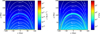 |
Fig. 1 Left: initial density configuration of the coronal loop. Right: initial pressure configuration showing enhanced pressure in the left foot point. The white lines show the B-field direction. |
3 Vertical loop oscillations
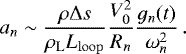
We run simulations for five different values of amplitude of the pressure enhancement corresponding to the values of the pressure contrast Π = 30, 40, 50, 70 and 100. In all cases, the pressure imbalance between the footpoints triggers a flow of material from the left footpoint to the right, as clearly seen in a time-distance plot of the density along the loop against time (Fig. 2). As the material approaches the right footpoint, it rebounds in the opposite direction. This process repeats with the material traversing the apex multiple times with decreasing speeds. The mechanism for this rebound is associated with the pressure build-up in the plasma close to the footpoints and with the action of the magnetic tension force resulting from bending of magnetic field lines and has been investigated in detail in Mackay & Galsgaard (2001) and Kohutova & Verwichte (2017a).
During the initial phase of the flow, the fast moving material travels past the loop apex at the maximum speed. The centrifugal force on the fast flowing plasma initially displaces the loop axis outwards. The restoring action of the Lorentz force pulls it back down resulting in an onset of a fundamental harmonic of a fast kink mode, as seen in the plot of the loop axis displacement determined as a function of distance along the loop. As seen from the time-distance plots of the location of the loop apex as a function of time shown in Fig. 3, there is a delay of ~ 300 s between the launch of the flow and the onset of the oscillation. This suggests that the excitation happens when the fast moving material first passes the apex of the loop. This is as expected taking into account the magnetic field geometry in our setup; the centrifugal force is inversely proportional to the radius of the curvature, which is greatest at the loop apex.
These oscillations are not predominantly caused by the overdensity at the loop apex as studied in Kohutova & Verwichte (2017b), despite the fact that a considerable mass of plasma is passing through the loop apex, as this would result in a downward displacement of the loop axis. Figure 4 shows that the loop axis is displaced outwards, suggesting that this effect is negligible compared to the effect of the centrifugal force. In order to analyse the loop oscillations, at each timestep wetake a cut along the centre of the domain perpendicular to the loop axis to create density time-distance plots. The loop apex displacement time series is obtained by fitting a Gaussian to the density profile at each timestep. We determine the loop oscillation parameters by fitting a sine function of the form ξ(t) = ξ0 sin(ωt + ϕ) to the loop displacement time series. The average oscillation period is ~340 s; although a slight modulation of the oscillation period is present for all pressure amplitudes, caused by the changes of the longitudinal density profile of the loop resulting from the motion of the flowing material along the loop axis (as studied in Kohutova & Verwichte 2017b). The amplitude of the oscillation varies from 0.7 to 2.2 Mm and increases with increasing pressure contrast at the footpoint, leading to faster flow velocity. The average speeds at which the flow passes the loop apex vary from 63 to 96 km s−1, while the sound speed at the loop apex is ~170 km s−1. We determine the kinetic energy density of the flow plasma using the average flow speed and the average density of the fast moving plasma at the apex. The dependence of the oscillation amplitude on the flow kinetic energy is approximately linear for small valuesof kinetic energy density and diverges from the linear regime for larger values (Fig. 5).
An estimate of the amplitude of the oscillation excited by the flow can be obtained by writing down an equation for a flow-driven kink oscillation:
![Mathematical equation: \begin{equation*} \Bigg[\frac{\partial^2}{\partial t^2} - C^2_{\mathrm{k}}\frac{\partial^2}{\partial s^2} \Bigg] \xi = \frac{\rho \mathrm{\Delta} s}{\rho_{\mathrm{L}} L_{\mathrm{loop}}} \frac{V_0^2}{R(s)} G(s,t) \, ,\end{equation*}](/articles/aa/full_html/2018/05/aa32656-18/aa32656-18-eq9.png) (8)
where Ck is the kink speed and the right-hand side represents the driving centrifugal force. Here V 0 is the average flow velocity, R(s) is the radius of the curvature of the loop as a function of distance along the loop, the ρΔ s∕ρLLloop term represents the mass of the plasma contained in the flow normalised by the total loop mass and G(s, t) is the shape of the flow pulse (to account for the fact that the flow due to the footpoint pressure difference is localised, as opposed to a uniform flow along the whole loop) represented by a dimensionless and normalised function of time and distance along the loop. The loop displacement ξ can be written as a superposition of normal modes ξ = Σan sin(kns). Similarly, G(s, t)∕R(s) = Σgn(t)∕Rn sin(kns). Equation (8) therefore becomes
(8)
where Ck is the kink speed and the right-hand side represents the driving centrifugal force. Here V 0 is the average flow velocity, R(s) is the radius of the curvature of the loop as a function of distance along the loop, the ρΔ s∕ρLLloop term represents the mass of the plasma contained in the flow normalised by the total loop mass and G(s, t) is the shape of the flow pulse (to account for the fact that the flow due to the footpoint pressure difference is localised, as opposed to a uniform flow along the whole loop) represented by a dimensionless and normalised function of time and distance along the loop. The loop displacement ξ can be written as a superposition of normal modes ξ = Σan sin(kns). Similarly, G(s, t)∕R(s) = Σgn(t)∕Rn sin(kns). Equation (8) therefore becomes
![Mathematical equation: \begin{equation*} \Bigg[\frac{d^2}{d t^2} - \omega^2_n \Bigg] a_n = \frac{\rho \mathrm{\Delta} s}{\rho_{\mathrm{L}} L_{\mathrm{loop}}} \frac{V_0^2}{R_n} g_n(t)\, , \vspace*{-3pt}\end{equation*}](/articles/aa/full_html/2018/05/aa32656-18/aa32656-18-eq10.png) (9)
where ωn is the mode frequency. This leads to the estimate of the mode amplitude given by
(9)
where ωn is the mode frequency. This leads to the estimate of the mode amplitude given by
 (10)
(10)
Assuming V 0 = 80 km s−1, g1 = 1 for a sine-like pulse, R1 = 90 Mm, ω1 =0.018 rad s−1 corresponding to oscillation periods of ~340 s. Δ s∕Lloop = 0.5 and ρ∕ρL ~ 10 results in the amplitude of the fundamental harmonic a1 ~ 1 Mm, which is in agreement with the simulation amplitudes.
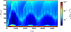 |
Fig. 2 Time-distance plot of the density along the loop averaged over 3 Mm in the direction perpendicular to the loop axis for Π = 50 during the first 5600 s. |
 |
Fig. 3 Time-distance plots at the loop apex for different values of footpoint pressure contrast. White solid lines show the centre of the loop profile determined by Gaussian fitting. Black dotted lines show best-fit sine function. |
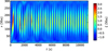 |
Fig. 4 Loop axis displacement from its original position as a function of time and position along the loop for Π = 50. |
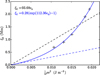 |
Fig. 5 Dependence of loop oscillation amplitude on kinetic energy density of the moving plasma at the loop apex. Solid blue line shows exponential fit to the data and dashed blue line shows linear expansion for small values of ϵk. Black dashed line shows linear fit to the data. |
4 Discussion and conclusions
The flows of plasma with speeds below 100 km s−1 are common in dynamic coronal loops (Teriaca et al. 2004; Doyle et al. 2006). We found that an impulsively driven flow with realistic speed is capable of exciting vertically polarised transverse loop oscillations with observable amplitudes ranging from a few hundred kilometers to 2 Mm, depending on the flow speed and the length of the loop. In addition to rapidly damped large-amplitude transverse loop oscillations excited by blast wave or a nearby flare and damping within few oscillation periods (e.g. Aschwanden et al. 1999; Nakariakov et al. 1999; White & Verwichte 2012), there are multiple observations of small-amplitude persistent transverse loop oscillations seen by SDO/AIA in quiet regions with no apparent excitation mechanism (Wang et al. 2012; Nisticò et al. 2013). These are typically explained by footpoint motions driven from the photosphere. In addition to the excitation of oscillations linked to thermal instability and coronal rain formation (Verwichte & Kohutova 2017; Kohutova & Verwichte 2017b), siphon flows (whether sustained or intermittent) therefore act as another possible excitation mechanism that can explain these small-amplitude sustained oscillations.
Pressure enhancement at one footpoint equivalent to enhancement in temperature can occur as a result of asymmetric footpoint-concentrated heating. Our problem could also, therefore, be set-up by enabling thermal conduction and heating one footpoint. Neglecting thermal conduction does not have a significant effect on the large-scale evolution of the loop and excitation of the oscillations, as verified by a test run for the Π = 50 case with the thermal conduction enabled. This is not surprising as the thermal conduction timescale τκ ~ L2nekB∕κ0T5∕2 is of the order of ~1000 s for coronal values used here and L = 10 Mm, which is long compared to the timescale on which the flow with average speed 100 km s−1 travels over the same distance τflow ~ 100 s. However, considering likely differences in the response of the loop plasma to the pressure enhancement once both thermal conduction and radiative losses are taken into account, the most accurate way to simulate flow velocities resulting from pressure imbalance would use a fully self-consistent approach including thermal conduction together with radiative losses and asymmetric footpoint heating. Furthermore, the nature of trigger mechanisms responsible for impulsive flows can be constrained with the help of observations focusing on the loop footpoints.
We note that we observed excitation of fundamental harmonic with the maximum displacement of the loop axis at the loop apex, in contrast to oscillations with maximum displacement in the loop legs reminiscent of second-order harmonic seen in Ofman et al. (2012). We attribute this difference to differences in the magnetic field configuration used in the two studies, with the radius of curvature of magnetic field lines being greater in coronal loop legs using our model.
It has also been proposed that the centrifugal force can result in excitation of transverse loop oscillations by fast moving coronal rain condensations formed in the loop as a result of thermal instability (Verwichte et al. 2017). However, the coronal rain blobs typically move with sub-ballistic speeds caused by pressure of the underlying plasma (Oliver et al. 2014; Kohutova & Verwichte 2017a) with only a small fraction having faster than free-fall speeds (Antolin & Verwichte 2011; Kohutova & Verwichte 2016). The fast speeds are typically explained by the blobs being accelerated by a background flow of the plasma (Müller et al. 2005; Fang et al. 2015). In this scenario, it is the combined effect of the fast moving cool blobs and the flow that can act as an oscillation excitation mechanism.
Acknowledgements
P.K. acknowledges the support of the UK STFC Ph.D. studentship. E.V. acknowledges financial support from the UK STFC on the Warwick STFC Consolidated Grant ST/L000733/I.
References
- Antolin, P., & Verwichte, E. 2011, ApJ, 736, 121 [NASA ADS] [CrossRef] [Google Scholar]
- Arber, T., Longbottom, A., Gerrard, C., & Milne, A. 2001, J. Comput. Phys., 171, 151 [NASA ADS] [CrossRef] [Google Scholar]
- Aschwanden, M. J., Fletcher, L., Schrijver, C. J., & Alexander, D. 1999, ApJ, 520, 880 [NASA ADS] [CrossRef] [Google Scholar]
- Cargill, P. J., & Priest, E. R. 1980, Sol. Phys., 65, 251 [NASA ADS] [CrossRef] [Google Scholar]
- Cargill, P. J., Spicer, D. S., & Zalesak, S. T. 1997, ApJ, 488, 854 [NASA ADS] [CrossRef] [Google Scholar]
- Doyle, J. G., Taroyan, Y., Ishak, B., Madjarska, M. S., & Bradshaw, S. J. 2006, A&A, 452, 1075 [NASA ADS] [CrossRef] [EDP Sciences] [Google Scholar]
- Fang, X., Xia, C., Keppens, R., & Van Doorsselaere T. 2015, ApJ, 807, 142 [NASA ADS] [CrossRef] [Google Scholar]
- Kohutova, P., & Verwichte, E. 2016, ApJ, 827, 39 [NASA ADS] [CrossRef] [Google Scholar]
- Kohutova, P., & Verwichte, E. 2017a, A&A, 602, A23 [NASA ADS] [CrossRef] [EDP Sciences] [Google Scholar]
- Kohutova, P., & Verwichte, E. 2017b, A&A, 606, A120 [NASA ADS] [CrossRef] [EDP Sciences] [Google Scholar]
- Mackay, D. H., & Galsgaard, K. 2001, Sol. Phys., 198, 289 [NASA ADS] [CrossRef] [Google Scholar]
- Mariska, J. T. 1988, ApJ, 334, 489 [NASA ADS] [CrossRef] [Google Scholar]
- Mariska, J. T., & Boris, J. P. 1983, ApJ, 267, 409 [NASA ADS] [CrossRef] [Google Scholar]
- McClymont, A. N., & Craig, I. J. D. 1987, ApJ, 312, 402 [NASA ADS] [CrossRef] [Google Scholar]
- Müller, D. A. N., De Groof, A., Hansteen, V. H., & Peter, H. 2005, A&A, 436, 1067 [NASA ADS] [CrossRef] [EDP Sciences] [Google Scholar]
- Nakariakov, V. M., Ofman, L., DeLuca, E. E., Roberts, B., & Davila, J. M. 1999, Science, 285, 862 [NASA ADS] [CrossRef] [PubMed] [Google Scholar]
- Nakariakov, V. M., & Roberts, B. 1995, Sol. Phys., 159, 399 [NASA ADS] [CrossRef] [Google Scholar]
- Nisticò, G., Nakariakov, V. M., & Verwichte, E. 2013, A&A, 552, A57 [NASA ADS] [CrossRef] [EDP Sciences] [Google Scholar]
- Ofman, L., Wang, T. J., & Davila, J. M. 2012, ApJ, 754, 111 [NASA ADS] [CrossRef] [Google Scholar]
- Oliver, R., Soler, R., Terradas, J., Zaqarashvili, T. V., & Khodachenko, M. L. 2014, ApJ, 784, 21 [NASA ADS] [CrossRef] [Google Scholar]
- Orlando, S., Serio, S., & Peres, G. 1994, Space Sci. Rev., 70, 203 [CrossRef] [Google Scholar]
- Priest, E. R. 1982, Solar Magnetohydrodynamics (Springer) [CrossRef] [Google Scholar]
- Teriaca, L., Banerjee, D., Falchi, A., Doyle, J. G., & Madjarska, M. S. 2004, A&A, 427, 1065 [NASA ADS] [CrossRef] [EDP Sciences] [Google Scholar]
- Terradas, J., Arregui, I., Verth, G., & Goossens, M. 2011, ApJ, 729, L22 [NASA ADS] [CrossRef] [Google Scholar]
- Tian, H., Curdt, W., Marsch, E., & He, J. 2008, ApJ, 681, L121 [Google Scholar]
- Tian, H., Marsch, E., Curdt, W., & He, J. 2009, ApJ, 704, 883 [NASA ADS] [CrossRef] [Google Scholar]
- Verwichte, E., & Kohutova, P. 2017, A&A, 601, L2 [NASA ADS] [CrossRef] [EDP Sciences] [Google Scholar]
- Verwichte, E., Kohutova, P., Antolin, P., Rowlands, G., & Neukirch, T. 2017, Proc. Int. Astron. Union, in press [Google Scholar]
- Wang, T., Ofman, L., Davila, J. M., & Su, Y. 2012, ApJ, 751, L27 [Google Scholar]
- White, R. S., & Verwichte, E. 2012, A&A, 537, A49 [NASA ADS] [CrossRef] [EDP Sciences] [Google Scholar]
All Figures
|
Fig. 1 Left: initial density configuration of the coronal loop. Right: initial pressure configuration showing enhanced pressure in the left foot point. The white lines show the B-field direction. |
| In the text | |
|
Fig. 2 Time-distance plot of the density along the loop averaged over 3 Mm in the direction perpendicular to the loop axis for Π = 50 during the first 5600 s. |
| In the text | |
|
Fig. 3 Time-distance plots at the loop apex for different values of footpoint pressure contrast. White solid lines show the centre of the loop profile determined by Gaussian fitting. Black dotted lines show best-fit sine function. |
| In the text | |
|
Fig. 4 Loop axis displacement from its original position as a function of time and position along the loop for Π = 50. |
| In the text | |
|
Fig. 5 Dependence of loop oscillation amplitude on kinetic energy density of the moving plasma at the loop apex. Solid blue line shows exponential fit to the data and dashed blue line shows linear expansion for small values of ϵk. Black dashed line shows linear fit to the data. |
| In the text | |
Current usage metrics show cumulative count of Article Views (full-text article views including HTML views, PDF and ePub downloads, according to the available data) and Abstracts Views on Vision4Press platform.
Data correspond to usage on the plateform after 2015. The current usage metrics is available 48-96 hours after online publication and is updated daily on week days.
Initial download of the metrics may take a while.