| Issue |
A&A
Volume 612, April 2018
|
|
|---|---|---|
| Article Number | A118 | |
| Number of page(s) | 12 | |
| Section | Interstellar and circumstellar matter | |
| DOI | https://doi.org/10.1051/0004-6361/201732073 | |
| Published online | 10 May 2018 | |
New insights into the outflows from R Aquarii
1
Tartu Observatory,
Observatooriumi 1,
Tõravere
61602, Estonia
e-mail: This email address is being protected from spambots. You need JavaScript enabled to view it.
2
Institute of Physics, University of Tartu,
Ravila 14c,
Tartu
50411, Estonia
3
GRANTECAN,
Cuesta de San José s/n,
38712
Breña Baja,
La Palma, Spain
4
Instituto de Astrofísica de Canarias,
38200 La Laguna,
Tenerife, Spain
5
Departamento de Astrofísica, Universidad de La Laguna,
38206 La Laguna,
Tenerife, Spain
6
Kapteyn Instituut,
Rijksuniversiteit Groningen,
Landleven 12,
9747AD
Groningen, The Netherlands
7
Observatorio Astronómico Nacional (OAN-IGN),
C/ Alfonso XII,
3,
28014
Madrid, Spain
8
Terroux Observatory,
Canberra, Australia
9
Astrophysics Research Centre, School of Mathematics and Physics, Queen’s University Belfast,
Belfast
BT7 1NN, UK
10
Nordic Optical Telescope,
Apartado 474,
38700
Santa Cruz de La Palma, Spain
11
Leiden Observatory, Leiden University,
Postbus 9513,
2300 RA
Leiden, The Netherlands
12
CNRS, UMR 7095, Institut d’Astrophysique de Paris,
98bis Boulevard Arago,
75014
Paris, France
Received:
10
October
2017
Accepted:
23
January
2018
Abstract
Context. The source R Aquarii is a symbiotic binary surrounded by a large and complex nebula with a prominent curved jet. It is one of the closest known symbiotic systems, and therefore offers a unique opportunity to study the central regions of these systems and the formation and evolution of astrophysical jets.
Aims. We aim to study the evolution of the central jet and outer nebula of R Aqr, taking advantage of a long term monitoring campaign of optical imaging, as well as of high-resolution integral field spectroscopy.
Methods. Narrow-band images acquired over a period of more than 21 yr were compared in order to study the expansion and evolution of all components of the R Aqr nebula. The magnification method was used to derive the kinematic ages of the features that appear to expand radially. Integral field spectroscopy of the [O III] 5007 Å emission is used to study the velocity structure of the central regions of the jet.
Results. New extended features, further out than the previously known hourglass nebula, are detected. The kinematic distance to R Aqr is calculated to be 178 pc using the expansion of the large hourglass nebula. This nebula of R Aqr is found to be roughly 650 yr old, while the inner regions have ages ranging from 125 to 290 yr. The outer nebula is found to be well described by a ballistic expansion, while for most components of the jet strong deviations from such behaviour are found. We find that the northern jet is mostly red-shifted while its southern part is blue-shifted, apparently at odds with findings from previous studies but almost certainly a consequence of the complex nature of the jet and variations in ionisation and illumination between observations.
Key words: binaries: symbiotic / circumstellar matter / ISM: individual objects: R Aqr / ISM: jets and outflows / ISM: kinematics and dynamics
© ESO 2018
1 Introduction
Symbiotic stars are interacting binaries composed of a hot component, usually a white dwarf, and a mass-losing red giant. The large mass loss from these evolved companions, the fast winds of the white dwarfs, and the occurrence of nova-like explosions, produce a rich circumstellar environment often taking the form of bipolar nebulae, collimated jets, or generally complex ejecta.
The source R Aquarii (R Aqr) is a symbiotic binary system, consisting of a M7III Mira variable and a white dwarf, surrounded by complex nebular structures extending across several arcminutes. At large scales, R Aqr appears as a bipolar, hourglass-like nebula with a prominent toroidal structure at its waist, within which a curved jet-like structure is found. At a distance of about 200 pc R Aqr is the closest known symbiotic binary, and therefore provides a unique opportunity to study in detail the evolution of a stellar outflows.
The hourglass nebula of R Aqr was first discovered by Lampland (1922) and repeated observations have revealed that it is expanding – at a first approximation – in a ballistic way (Solf & Ulrich 1985). The expansion of the large-scale nebula was used by Baade (1944) to calculate a kinematical age of 600 yr. Solf & Ulrich (1985) refine this value to 640 yr by applying a kinematical model using a hourglass geometry, with an equatorial expansion velocity of 55 km s−1, and assuming that the expansion velocity at each point of the nebula is proportional to the distance from the centre.
The presence of the central jet in R Aqr was first remarked upon by Wallerstein & Greenstein (1980), however Hollis et al. (1999a) showed that the jet was present in observations taken as early as 1934. Since these earlier observations, the large-scale S-shape of the jet has remained unchanged, while at smaller scales its appearance has varied greatly even on short timescales (Paresce et al. 1991; Michalitsianos et al. 1988; Hollis et al. 1990, 1999b; Kellogg et al. 2007, this work). A detailed investigation of the innermost 5″ of the jet has been carried out using high resolution radio data (e.g. Kafatos et al. 1989; Mäkinen et al. 2004). However, it has been demonstrated that at different wavelengths the appearance and the radial velocity pattern of the jet varies dramatically (Paresce et al. 1991; Hollis & Michalitsianos 1993; Sopka et al. 1982; Solf & Ulrich 1985; Hollis et al. 1990, 1999b).
In this article, we present a detailed study of the R Aqr nebula based on deep, narrow-band emission line imaging, acquired over a period of more than two decades, as well as on high spectral resolution integral field spectroscopy of the [O III] 5007 Å emission from the central regions. The data and data reduction is presented in Sect. 2, with the image processing techniques employed in our analysis in Sect. 3. Sections 4 and 5 contain the results of our analysis of the multi-epoch imaging, while Sect. 6 is dedicated to the results from the integral field spectroscopy. Finally, in Sect. 7, we present our conclusions.
2 Observations and data reduction
2.1 Imaging
The imaging data presented in this paper was collected over more than two decades at various observatories. Most of the data were obtained with the 2.6 m Nordic Optical Telescope (NOT) using the Andalucia Faint Object Spectrograph and Camera (ALFOSC). ALFOSC has a pixel scale 0.″19 pix−1 and a field of view (FOV) of 6.′4 × 6.′4. Previously, in 1991, we obtained a single Hα+[N II] image with European Southern Observatory’s (ESO) New Technology Telescope (NTT) equipped with ESO Multi-Mode Instrument (EMMI, 0.″35 pix−1 and a FOV of 6.′2 × 6.′2; Dekker et al. 1986). More recent data were obtained in 2012 with ESO’s Very Large Telescope (VLT) and its Focal Reducer/low dispersion Spectrograph 2 (FORS2; Appenzeller et al. 1998). The standard resolution collimator of FORS2 was used resulting in a pixel scale of 0.″25 pix−1 and a FOV of 6.′8 × 6.′8. At all epochs several narrow-band filters were used. Due to the moderate radial velocities present in the R Aquarii jet and bipolar nebula, all filters include all the light from corresponding emission lines, except the 2002 [N II] filter which only includes radial velocities larger than +45 km s−1considering the [N II] 6583 Å rest wavelength. Filters centred at Hα also include emission from the [N II]λλ6548, 6583 Å doublet. Details of the central wavelengths (CW) and full widths at half maxima (FWHM) of all filters employed, as well as other observational details can be found in Table 1. As can be seen from the table, most of the data were taken with the NOT+ALFOSC, under good seeing conditions. Airmass mostly never exceeded 1.5. This allows safe comparison of this homogenous set of images. All the individual frames were reduced (bias, flat field correction) using standard routines in IRAF1.
An additional set of deep observations was obtained on October 2, 8, and November 2, 3, 2016 in Terroux Observatory, Canberra, Australia using a 30 cm f3.8 Newtonian telescope with a CCD camera and narrow-band [O III] (5010 Å, FWHM = 60 Å) and Hα (6560 Å, FWHM = 60 Å) filters. The pixel scale was 0.″84 pix−1. We obtained 34 frames for a total exposure time of 7.6 h in [O III], while 32 frames adding up to 6.8 h were taken in Hα. Frames were flat field corrected and median combined.
2.2 Spectroscopy
Integral field unit (IFU) spectroscopy was obtained on October 3, 2012, with the VLT equipped with the Fibre Large Array Multi Element Spectrograph FLAMES (Pasquini et al. 2002) in GIRAFFE/ARGUS mode. The ARGUS IFU provides continuous spectral coverage for a 11.″4× 7.″3 FOV (formed from an array of 0.″52 lenslets). The high resolution grating HR08 was used in the spectral range from 4920 Å to 5160 Å, covering both [O III] lines at 5007 Å and 4959 Å. The spectral reciprocal dispersion was 0.05 Å pix−1. Observations were acquired at four different pointings in order to cover the inner region of the jet (see [O III] frame in Fig. 1). All data were reduced using the ESO GIRAFFE pipeline v2.9.2, which comprises debiasing, flat-field correction and wavelength calibration. Individually reduced exposures were then combined to produce a master data cube for each pointing. A log of the VLT+FLAMES observations is presented in Table 2.
3 Image processing
To allow a careful study of the proper motions of nebular features over the whole monitoring period, it was necessary to map all images to the same reference frame. The first step was to find the astrometry solution of each frame. Owing to the lack of suitable field stars near R Aqr (particularly problematic in short exposures taken with very narrow-band filters), the field geometric distortions and rotationin the NOT and VLT frames were computed from more populated fields observed with the same filters. Those fields were observed as close to the R Aqr observations in time as possible in order to minimise the impact of any long-term effects. The analysis allowed us to conclude that the adopted filters do not introduce additional geometric distortions and that a common astrometric solution can be obtained. Astrometric solutions were calculated using the tasks ccmap and ccsetwcs in IRAF and applied to the R Aqr data using the python based Kapteyn package (Terlouw & Vogelaar 2015). Errors in the astrometric solutions were on average 0.″19 ± 0.″07. No less than 50 stars per field were used, occasionally up to 200. For the NTT 1991 images it was not possible to obtain a precise astrometric solution at this stage.
As a second step, all images were matched against a reference frame in all filters (data with * in Table 1) using the stars in the FOV other than the R Aqr central star. This step was needed in order to place all frames onto the same pixel scale for a direct pixel-to-pixel comparison. The IRAF tasks geomap and geotran were used to perform the matching. With this step, all the frames were resampled to the scale of the reference frame, namely 0.″19 pix−1. The RMS of the matching for [O III], Hα+[N II], and [N II] images was mostly smaller or equal to 0.″07. For the 1991Hα+[N II] image, the matching errors were σRA = 0.″12, σDec = 0.″11. In [O II], only afew field stars are available, and therefore we adopted the matching solution from the [O III] frame obtained on the same night. An a posteriori check using the few field stars available suggests a matching error generally below 0.″08 for this filter. In the case of the 1997 [O II] frame, there were no [O III] observations acquired, and consequently a solution was found directly from the five field stars available. The matching errors were σRA = 0.″09, σDec = 0.″12.
Considering the large time spanned by our data, the possible influence of proper motions of field stars used for astrometry was also investigated. Proper motions were taken from the USNO-B1.0 catalogue (Monet et al. 2003), or from the UCAC4 catalogue (Zacharias et al. 2013) if measurements from the former were not available. We conclude that the corresponding errors in the matching of the images are negligible.
A correction for the proper motion of the central binary star of R Aqr itself, which is non-negligible over the period considered given the proximity of the system, was then applied. We measured the proper motion directly in all non-saturated images, while the value of the proper motion from UCAC4 (μRA = 29.5 mas yr−1, μDec = −32.1 mas yr−1) was used for the saturated frames. Finally, all images were aligned with respect to the central star using the frame obtained on September 5, 2007 as a reference.
Log of the imaging data.
Log of the VLT+FLAMES spectroscopic observations.
4 Overall properties of the R Aqr outflows
The R Aqr outflow consists of a bright, curved jet structure contained within a larger bipolar nebula (Hollis et al. 1990). The inner regions of the jet extend along the north-east to south-west direction, at an apparent angle of 40 degrees from the symmetry axis of the bipolar lobes which instead are very close to the north-south orientation.
Solf & Ulrich (1985) also identified an inner bipolar nebula, orientated along the same symmetry axis as the larger lobes but on a smaller scale. However, this latter structure is not obviously visible in any of our images. Figure 1 shows the large-scale morphological properties of these outflows and the faint new details revealed by our deep imaging.
4.1 Structure and expansion of the bipolar nebula
The large system of lobes and their bright equatorial waist are mainly visible in the lower-ionisation light of Hα+[N II], [O II], and [O I] (Fig. 1). Indeed, Gonçalves et al. (2003) show large [N II]/Hα and [S II]/Hα flux ratios in the ring of the bipolar nebula that they ascribed to shock ionization.
The appearance of the ring and lobes, at the high resolution provided by our images, is complex. In the light of low-ionization ions, the ring is broken into knotty and filamentary structures, while it appears much smoother in the light of higher ionization species such as [O III]. Furthermore, our deep images show for the first time fainter features that we designate as streams in Fig. 1. Streams appear in the NE and SW direction of the bipolar lobes extending up to 1.′2 from the central star. On the southern side, the streams seem to replicate the curved appearance of the outer regions of the jet.
The overall structure of the bipolar nebula does not show notable changes over the 21 yr considered (1991–2012). We therefore use the so-called magnification method (see Reed et al. 1999; Santander-García et al. 2007) to calculate the expansion in the plane of the sky and hence the age of this structure. The essence of the method is to find the magnification factor, M, that cancels out residuals in the difference image obtained by subtracting the first epoch, magnified image from the second epoch image. The method assumes homologous expansion of the structure, but also allows one to identify deviations from this assumption.
The magnification factor was found using the 1991 and 2012 Hα+[N II] images. Owing to the different instruments, filters properties, and observing conditions, we matched the point-spread function of images using field stars, and we also rescaled them in brightness using a portion of the nebula itself. Increasing magnification factors were then applied to the 1991 frame, and the differences with the 2012 image computed. A precise determination of the best-fitting magnification factor is limited by the highly inhomogeneous morphology of the nebula. By dividing the nebula into quadrants, we found that the best-fitting M values were as follows: NE 1.030, SE 1.033, SW 1.033. Due to the faintness of the NW region of the nebula no measurement could be obtained from that quadrant, and for this reason we also defined a W region restricted to the prominent part of the waist in that direction where a value of 1.033 to 1.036 was derived.
Assuming that the nebula has grown in time at constant velocity, the resulting nebular age, computed with respect to the first epoch, is T = Δt∕(M − 1), where Δt is the time lapse between the two epochs, in our case 21.17 yr. The M values above imply an average age, weighted by errors, of the bipolar nebula of Tbip = 653 ± 35 yr in 1991, which compares well with previously published results (see Sect. 1). Yang et al. (2005) find that R Aqr could have experienced a nova explosion in A.D. 1073 and A.D. 1074. Without knowing the initial conditions of the explosion and of the circumstellar medium (ISM) it is not possible to find further support to the relation between the bipolar nebula and the possible ancient nova outburst, nor to discard it.
The estimated ages of the SW streams indicate that they are likely part of the extended nebula, rather than jet features. The stream in the NE is not detected in our 1991 Hα+[N II] image therefore no age estimate can be given.
An additional set of images acquired in the Terroux Observatory reveal new faint outer features in [O III] and in Hα. A combined [O III] and Hα image is presented in Fig. 2. It reveals the existence of a thick [O III] arc along the east-west direction with an extent of 6.′4, and a thinner and fainter Hα loop, which extends to the north up to 2.′8 from the central source. The latter may be related to the streams described in the previous section.
The [O III] arc is confirmed by stacking up all our other [O III] and [O II] long exposure frames, but at a low signal-to-noise ratio. Unfortunately, the Hα feature is undetected in our VLT images, as their FOV does not fully cover the region. It is likely that these features are related to the mass loss from the red giant and/or a nova eruption from the white dwarf in the earlier evolutionary stages of the system.
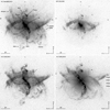 |
Fig. 1 VLT 2012 Hα+[N II], [O II], [O III] and NOT 2009 [O I] frames. On the [O III] frame the white boxes represent the spectroscopic observations (see Sect. 2.2). The FOV of all frames is 3′ × 3′. North up, east left. |
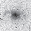 |
Fig. 2 Terroux image showing faint outer [O III] and Hα features. FOV = 9′× 9′. See text for further details. |
4.2 Kinematic distance
The combination of our determination of the apparent expansion of the bipolar nebula with the radial velocity measurements of Solf & Ulrich (1985) allows us to derive the expansion parallax of R Aqr nebula. In particular, Solf & Ulrich (1985) found that the equatorial waist can be modelled as an inclined ring expanding at a speed of Vexp = 55 km s−1.
The angular expansion of matter along the major axis of the projected ring, over the period Δt considered, is Δα = α(M − 1), where α is the distance from the central source of the intersection of the ring with the plane of the sky. Knowing the linear speed Vexp, the distance to R Aqr follows immediately from the relation (in convenient units)
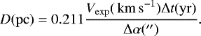 (1)
(1)
Adopting the average value of the magnification factors determined above, and fitting an ellipse to the nebular ring to measure its major axis, we obtain a kinematic distance to R Aqr of 178 ± 18 pc. In general, this kinematic distance is in fair agreement with previous estimates. The nebular kinematics were first used by Baade (1944) to derive a distance of 260 pc, later revised down to 180–185 pc (Solf & Ulrich 1985). This value is also in good agreement with the estimate of 181 pc by Lepine et al. (1978) based on the absolute magnitude of R Aqr at 4 μm and an assumed value of −8.1m. HIPPARCOS parallax measurements by Perryman et al. (1997) result in a slightly larger distance of 197pc, in strong agreement with the estimate based on the separation of the orbital components measured by the VLA (Hollis et al. 1997b). More recently, parallax measurements of SiO maser spots using VERA have indicated a yet greater distance of 214–218 pc (Kamohara et al. 2010; Min et al. 2014).
5 Structure and expansion of the jet
Unlike the large-scale bipolar nebula, which within our present errors in the determination of the apparent and radial motions is well modelled assuming a mainly ballistic expansion, the jet shows a much more complex and irregular evolution. In our images, features identified by previous authors have brightened or faded, or even broken into multiple components moving along different directions. The bulk motions of various regions of the jet determined using our images are highlighted in Fig. 3. They demonstrate that, while the overall flow pattern is consistent with a radial expansion of the jet, in some regions there are significant deviations, even perpendicular the radial direction of expansion. Their complex changes of appearance are probably the combination of illumination and/or ionisation variations, and shocks. This makes the magnification method inappropriate to describe them. To illustrate this, we will discuss the evolution of individual features across our multi-epoch imagery in the following sub-sections.
Figures 4 and 5 show the evolution over time of the northern and southern region of the jet in the most relevant epochs and filters. We note that the bright central area is often saturated, with strong charge overflow especially in Hα+[N II]. The intensity level of the different frames in both figures was adapted to maximize the visible information. The small blob near the central source in the [O II] 2007 and 2009 frame, pointed to with arrows in Fig. 4, are a red-leak images of the central star (displaced because of atmospheric differential refraction at the significant airmass of these observations). In Fig. 5 on the 2009 [O III] frame, instrumental artefacts are visible as faint lighter thick lines emanating from the central star at PAs 135° and 225°.
In order to avoid confusion, some clarification of the nomenclature of the jet features used in the past is in order. We refer to the earliest designated jet features from Sopka et al. (1982, hereafter referred to as SHKM) as BSHKM, CSHKM, and the “loop”. Later publications revealed more details of the jet closer to the central source, which were designated as knots A and B by Kafatos et al. (1983), and knot D and S by Paresce et al. (1988). Knot S is a brightness concentration inside the loop feature and is therefore often referred to as loop+S. We keep the designations of the later authors. The aforementioned features, as well as the new ones found in this work, are indicated in Figs. 1, 3–5.
Most of our images, as well as previously published data (imaging and spectra), show that the NE jet is brighter than the SW jet at both large scale and in the central area (Paresce & Hack 1994). However, our short exposure [O III] and [O II] VLT images from 2012 reveal that in the central region (<2″), the SW jet is brighter. This is also confirmed by our spectral data from 2012 (Fig. 7). This seems to have appeared a few years before 2012, as the images from 2002 and 2007 show equal brightnesses for NE and SW in the central area, while by 2009 and 2012 clearly the SW is more prominent. This central area is resolved in the recent high spatial resolution SPHERE images from 2014 by Schmid et al. (2017). They also detect that the SW jet is brighter than its NE counterjet in these central areas.
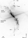 |
Fig. 3 NOT 2007 [O III] image, with logarithmic display cuts that highlight the overall structure of the jet. Arrows point the expansion direction. FOV is 1.′5 × 2.′0. |
5.1 The NE jet
The evolution of the northern, bright part of the jet is shown in Fig. 4. It has a complex, knotty, and variable appearance. For instance, the feature that we name F first appeared in 2007 in the [O III] filter. The 2012 image indicates that, contrary to the general radial expansion, it is seemingly moving towards the west. The same applies to feature G, which appeared in 2011. Their westwards lateral movements are indicated by the two arrows in Fig. 3. Transformed into linear velocities, their motions would imply speeds of between 500 and 900 km s−1. This is several times larger than the bulk radial motions from imaging and spectroscopy, indicating that very likely they do not reflect the true physical movement of a clump of material but rather are due to changes in the ionisation conditions of the region.
At a distance of ~20″ (see Fig. 3) the northern jet splits into two components, a brighter one bending towards the north and ending in filamentary features such as CSHKM and NE4, and a fainter, more diffuse one that seems to be a straight, conical extension of the innermost jet. The latter is only visible in the [O III] emission line and its cone-like morphology suggest that it may be an illumination effect (Corradi et al. 2011), further indicating that the role of changing illumination/excitation is critical in understanding the structure of the jet.
Burgarella & Paresce (1991) used optical emission line ratios to conclude that the R Aqr jet features are best fitted with local shock-wave models, as was first suggested by Solf & Ulrich (1985). Burgarella & Paresce (1991) found that the brightening of knot D (and fading of knot B) came some 15 yr after the brightening of knot B (in the late 1970s), concluding that the shock wave was propagating outwards at 90–100 km s−1. As such, they predicted that the knot D should fade analogously 15 yr after it was observed to brighten, which would approximately occur in 2003. Inspection of our Hα+[N II] data, Fig. 4, reveals that in 1991 B and D have similar brightness (just as in observation from 1986 in Burgarella & Paresce 1991). Our next Hα+[N II] frame is from 2009 were knot D, indeed, is much fainter than knot B, while at the same time the knot A is the brightest. By 2012, the relative brightness of knot B is around that of knot A, while knot D is the faintest. A similar tendency is detected in our [O II] data where by 1997–2002 knot B has almost disappeared, while knot A and D are clearly brighter. By 2007 knot B starts to brighten again and quite soon (2009) becomes as bright as knot A. At the same time it does appear that knot D is fading. The similar relative brightening of knot B is visible in the [O III] frames. To conclude, the prediction of knot D fading is confirmed (though perhaps at a faster rate than predicted). In addition, the re-brightening of knot B may imply that another shock wave is passing through the system. If so, it should eventually start again influencing knot D. However, from Fig. 4 it is evident that, by our latest epochs, knot B has stretched as far out as knot D, but the latter is not brightening together with knot B.
Over the years, features in the central area of the NE jet (Fig. 4) tend to get elongated along the expansion direction and eventually break into separate components. For instance, feature B breaks into B1 and B2. Similar stretching is happening with features A and D, which was seen to happen at 8 GHz radio band as early as 1992 (Mäkinen et al. 2004). Our data shows that by 2012 in all filters feature A has a very elongated structure, which is clearly indicative of imminent breakup. The delay between optical and radio can be just due to the lower resolution available in optical wave bands.
As indicated by the arrows in Fig. 3, the outermost NE jet features expand radially during the period considered. Therefore we use the magnification method (features CSHKM and NE4, see Fig. 1) or measure directly the proper motion (feature BSHKM, Figs. 1 and 4) to estimate their kinematical ages. The ages together with approximate distances from the central star are presented in the Table 3. Ages are presented for the epochs 1991-07-06 and 2012-09-05. The distances are measured at the 2012-09-05 date because not all features were present on the 1991 image. Due to the extended nature of most of these features, distances from the central source are roughly estimated. Details relating to the measuring can be found in Appendix A. Here only the main results are presented.
The measurements of the brightness peak of feature BSHKM indicate an age between 125 and 180 yr. The average proper motion, μ = 0.″10 ± 0.″02 yr−1, is compatible with the calculations in SHKM (0.″082 ± 0.″014 yr−1), indicating a roughly constant expansion velocity over the last 50 yr or so. Feature CSHKM was twice as bright in 2012 than in 1991. In SHKM, a slow brightness change for that feature is mentioned, but it is not clear if it was observed to be brightening or dimming. The age found for that feature, 286 yr, is much younger than the bipolar nebula, though much older than the previously derived jet age of about 100 yr (Lehto & Johnson 1992; Hollis & Michalitsianos 1993). If the CSHKM feature is part of the jet, it is not surprising that the brightness has changed, as brightness variations have been seen among all features of the jet. The feature also demonstrates the jet’s structural differences at different wavelengths, given that CSHKM keeps its structure in time when considering single filter data, but its form varies in different filters. In Hα+[N II] it has an arched shape, while in [O III] it seems a double arched or circular. In [O I] it has a T-shape structure. For feature NE4, an age of 285 ± 61 yr is found. This age is much younger than the bipolar nebula, though older than the jet, just as found for CSHKM. Collectively our observations of BSHKM, CSHKM, and NE4 imply that they are real physical structures, and that their apparent morphological changes are not dominated by the changing ionisation.
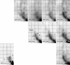 |
Fig. 4 NE jetin [O II], [O III], and Hα+[N II] frames from top to bottom respectively. One square is 5″ × 5″. The FOV of each frame is 20″ × 30″. North is up, east to the left. |
5.2 The SW jet
The evolution of the SW jet from 1991 to 2012 in the most relevant filters is presented in Fig. 5. We refer to the SW jet with the following nomenclature. SW1 consists of several blobs (apart from the loop+S) seen in the 1991 Hα+[N II] frame in Fig. 5. The rest of the SW jet visible in Fig. 5 is named SW2. The more extended features SW3 and SW4 are also highlighted in Fig. 1. The expansion of the SW jet is more uniform than the northern one, showing mostly radial motions (features loop+S, SW4, and SW3 in Figs. 1 and 5). However, we are able to make a few interesting remarks based on our observations.
First of all, the relative brightness of SW2, compared to SW1, has increased over the years. The complex was marginally visible in our 1991 Hα+[N II] frame, and overall is now as bright as SW1. Significant structural changes are also detectable in the SW2 (compare 1997 and 2002 [O II] in Fig. 5), and more structure has become visible which seems to connect SW2 with SW3 via faint curved filaments (see Fig. 1).
Feature H, shown in the light of [O III] in Fig. 5, is found to be moving faster than the surrounding jet at the epochs 2002, 2007, 2009, and then disappears or dissolves into the surrounding jet emission. Its proper motion is on average 0.″30 ± 0.″01 yr−1. Taking into account the distance to R Aqr found in Sect. 4.2 the average linear velocity would be ~ 250 km s−1. This is not as fast as the lateral movements detected in the NE jet but it is still faster than the jet in general, again possibly resulting from a shock wave moving through the system rather than a real matter movement. If we assume constant velocity, it was ejected 38 ± 1 yr ago.
In the SW jet, kinematical ages could be calculated using the magnification method for the radially expanding features loop+S, SW3, and SW4 (see Figs. 1 and 5). As for the NE jet, details of the analyses are presented in Appendix A and Table 3. The feature looppreserves its horseshoe shape over our observing period in all filters in which it is detected. The brightness enhancement, knot S, was detected in 1986 by Paresce et al. (1988) is still clearly visible in our 1991 Hα+[N II] frame (see Fig. 5). At later epochs, the knot S becomes elongated along the loop until it almost disappears, but that part of the loop stays brighter than the other regions. Figure 5 also shows that the loop is slowly expanding towards the south. The age found for the loop+S, 160 yr, corresponds to an ejection event around the year 1827 ± 40. This is comparable with the ejection date 1792 ± 32 computed by SHKM. This also shows that no major changes have occurred in the evolution of the loop since their observations in the 1960s. The estimated age of feature SW3, 215 ± 36 yr is much younger than the bipolar nebula, though older than the jet, just as found for NE4 and CSHKM. In the case of the newly-identified hook-shaped feature SW4 we find a rather large age value (880 ± 150 yr) but as the feature is very faint, we conclude that its age is consistent within the uncertainties with that of the extended bipolar nebula. The age of the ballistic features of the jet increases with the distance from the centre, consistent with continuous or repeated ejection events or that the more extended features have been slowed down by circumstellar material.
Kinematic ages at epochs 1991-07-06 and 2012-09-05 together with an approximate distances for the epoch 2012-09-05 from the central source for the ballistic features of the jet.
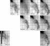 |
Fig. 5 SW jet in [O II], [O III], and Hα+[N II] frames. One square is 5″ × 5″. The FOV of each frame is 20″ × 30″. North is up, east is left. |
6 Radial velocity measurements
The [O III] 5007 Å emission extends over the entire FOV of the ARGUS IFU pointings, except for very few spaxels. This resulted in ~1200 usable individual spectra in total. Radial velocity measurements were obtained from each lenslet by Gaussian fitting of the [O III] line using the splot task in IRAF. Every fit was visually checked and multiple Gaussians were used when needed. The measured radial velocities were corrected first to the local standard of rest (LSR), and then to R Aqr systemic velocity of −24.9 km s−1 (Gromadzki & Mikołajewska 2009).
The [O III] line profiles are generally complex and sometimes display broad wings, as illustrated in Fig. 6. We initially limited the discussion to the strongest emission peaks, defined as those spectral components whose integrated flux is larger than 75% of any other component from the multi-Gaussian fit at each spaxel. Results are presented in Fig. 7, where the radial velocities of the strongest peaks are plotted on top of the reconstructed [O III] image.
At position 1 (POS1, see Fig. 6), that is centred on the star, the radial velocity varies from −33 to +72 km s−1, with the innermost portion of the south jet being blueshifted, and the north counterpart mainly redshifted. This trend continues further away from the centre, at position 2 (POS2, to the north) that is mostly redshifted (from −5 to +97 km s−1) and position 3 (POS3, to the south), which is mostly blue-shifted with a few redshifted components (from −56 to +59 km s−1). At position 4 (POS4), where the southern jet significantly bends, most of the emission becomes redshifted, ranging from −38 to +137 km s−1. This general description is obviously complicated by the very complex line profiles, which include additional emission components as well as extended wings spanning a range of radial velocities as large as ~ 400 km s−1. In general, however, it is clear that on the same side of the central star, both red- and blue-shifted regions are found, which – assuming purely radial motions – is a clear sign of a changing direction of the ejection vector crossing the plane of the sky. This in turn is usually associated to precession of the ejection nozzle as seen at large inclinations.
From Fig. 7 it is evident that broken up components of feature B, namely B1 and B2 (see Sect. 5.1), have different radial velocities, VradB1 = +73 ± 27 km s−1 and VradB2 = +22 ± 22 km s−1, respectively. Similarly, we calculate their average FWHM to be 78 ± 23 km s−1 and 32 ± 24 km s−1, respectively. As such, B1 presents almost three times the radial velocity of B2 and nearly twice its velocity dispersion. From their motion in the plane of the sky, we see that the entire feature B (including components B1 and B2) has been moving steadily towards the NE (Fig. 3), implying that their velocities in the plane of the sky should be similar. As such, we can conclude that the true spatial velocity of B2 is significantly lower than that of B1.
Another feature for which we can determine a radial velocity from the data shown in Fig. 7is feature F (see Sect. 5.1). It has a uniform radial velocity over the whole elongated feature, + 36 ± 2 km s−1, with a narrow single Gaussian line profiles FWHM = 16 ± 1 km s−1. This would seem to imply that the feature F is moving almost completely perpendicular to the line of sight, as its tangential velocity, 500 km s−1(see Sect. 5.1), is much larger than the measured radial velocity.
In an attempt to clarify the overall Doppler-shift kinematics of the jet, and compare with previous observations, we have extracted from the 3 ARGUS data cubes surrounding the central star a position-velocity plot simulating an observation with a long slit, with a width of 1 arcsec, orientated along the general orientation of the jet at PA = 40°, and through the central source (Fig. 8). Hollis et al. (1990) adopted instead PA = 29°, which was aligned with the inner jet at that time. Considering the overall PA change of the jet between the Hollis et al. (1990) and us (about 30 yr later) it clearly indicates that the jet, on large scales, is rotating counterclockwise (CCW). The CCW evolution of the jet has also been seen in radio observations (Hollis et al. 1997a).
The extracted longslit (Fig. 8) confirms the overall structure of the jet. However, the figure also highlights the complex variation in velocity profile along the jet. A simple, ballistically-expanding, precessing jet would produce a perfect S-shape, while here we have an overall S-shape but with dramatic variations in the width of the S along the slit (much broader in the NE, perhaps reflective of the multiple components like B1 and B2, and with significant tails out to very high velocities). The SW jet, on the other hand, appears more regular in terms of velocity structure but much more broken spatially with “gaps” in the emission. Furthermore, the artificial long slit spectrum also highlights the acceleration in the inner parts of the jet (POS1). This is consistent with the solution proposed in Mäkinen et al. (2004) that the jet features, after being formed due to increased matter flow at periastron, are accelerated inside the first 1″ and then ejectedas bullets. The outer parts, POS2 and POS3, seem to expand freely. What is unclear throughout the length of the longslit is the contribution of illumination effects – perhaps the matter and velocity structure of the two sides of the jet are symmetricaland the observed differences are the result of differing illumination. The possible illumination beam visible on the [O III] 2007 and 2012 images in NE direction does not seem to move or, at most, moves very little. However, the cone is not seen in the southern direction indicating that this may be an important factor in determining the structure of the observed position-velocity profile.
When comparing our RV data with previously published data, at a first sight it seems that there is a notable and intriguing difference. We find that the NE jet is mostly red-shifted and the SW jet mostly blue-shifted, with occasional opposite velocity signs. Only in the furthest part of the SW jet covered by our IFU data, a significant redshifted component is detected.
Previously published data seem to indicate the contradictory behaviour, that is discussed in the following. A direct comparison with the RV data of SHKM is difficult because they do not mention if their radial velocities are corrected for the systemic velocity. Contrary to our findings, Solf & Ulrich (1985) found that the southern jet is mostly red-shifted and the northern one blue-shifted. Also, they measured radial velocities for features A and B of around −55 km s−1 (based on an [N II] 6583 Å emission line spectrum), which have an opposite sign compared to our measurement for feature B +20 to +70 km s−1 with respect to the systemic velocity. Only near the central star is there some agreement with our measurements, as Solf & Ulrich (1985) found a negative radial velocity, −20 km s−1, in the southern jet. Overall, Solf & Ulrich (1985) say that the southern jet is red-shifted and the northern blue-shifted but if one looks more carefully at their Fig. 5 it is evident that Solf & Ulrich (1985) have red- and blue-shifted components present at almost all measured positions.
Hollis et al. (1990) present long slit observations of the same emission line as we ([O III] 5007 Å) but also find that overall the NE jet peak emission is approaching and the SW receding, contrary to our measurements. Though, it is clear from their Fig. 1 that in the NE up to 7″ from the centre both blue and redshifted components are equally bright. Reconstructing their slit on our earlier data we see that most of their SW faint structure is somewhere at our POS4, which is also red-shifted. Hollis et al. (1999b) employed a Fabry-Perot imaging spectrometer to obtain velocity maps of the [N II] 6583 Å emission line, again finding that the northern jet is blue-shifted and the south red-shifted. They, too, remark that the FWHM is extremely large (up to several hundred km s−1) and that the velocity structure at each position is complex, often presenting multiple components – just as we find in our data.
Considering all the above mentioned observations and the nature of our measurements, the apparent discrepancies may be explained by brightness variations of the different line profile components, which would cause that, for example, a previously faint blue component has become significantly brighter than its red component. Furthermore, the higher spectral resolution of our data would allow us to better define the characteristics of the outflow for different components.
It is unlikely that the differences in radial velocity measurements with previous epochs are mainly due to precession effects, given the long ~2000 yr processing period (Michalitsianos et al. 1988).
We conclude that, at the intermediate scales of the R Aqr jet investigated in this article, most of the observed changes in the morphology and velocity are driven by changes in the illumination and ionising conditions of circumstellar gas at the different epochs of observations, as well as of local dynamical effects, rather than to a structural change of the entire jet of R Aqr.
Only in the innermost regions, significant structural changes are observed, as shown by Schmid et al. (2017). In these regions, some of the discrepancy with the RV data between different authors could indeed be related to the actual motion of the ionised material. The discrepancies that Schmid et al. (2017) find gives further indication of the complexity of the R Aqr system.
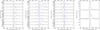 |
Fig. 6 Line profile examples from left to right POS1, POS2, POS3, and POS4. Blue vertical line refers to a radial velocity 0 km s−1. All radial velocities are corrected for the systemic velocity. |
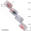 |
Fig. 7 Radial velocities of the emission peaks, superimposed onto a grey-scale representation of the reconstructed [O III] image from the IFU data. The FOV = 40″ × 40″. Radial velocities are indicated by lines, whose colour indicates if emission is blue- or red-shifted, and whose length is proportional to the absolute value of the velocity. Cyan and pink lines represent blue shifted velocities smaller than −5 km s−1 and redshifted smaller than +5 km s−1respectively. The length of the cyan and pink lines are constant because otherwise they would be too small to be visible. The white X-point marks the position of the central star. The distance used for the linear size is taken from this work: 178 pc. |
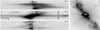 |
Fig. 8 Left: extracted long slit spectra with the PA = 40°, extending 18.″7 from the central star in both direction. The black vertical line is the 0 km s−1 radial velocity. In POS1 also the spectrum of the central star is visible. Right: the extracted long slit shown over the VLT pointings on top of a matched VLT [O III] frame. The central star is heavily saturated. The FOV is 30″ × 30″, north is up, east is left, slit width is 1″. |
7 Conclusions
We have presented a multi-epoch morphological and kinematical study of the nebula of R Aqr. New morphological features (referred to as the arc and loop) outside the known hourglass nebula add richness and complexity to the circumbinary gas distribution and the mass loss history from the system.
The large bipolar nebula of R Aqr is expanding ballistically and does not show major structural changes during the observed period. An average age of it was calculated to be Tbip = 653 ± 35 yr in 1991. Determination of its apparent expansion allows us to determine a distance to R Aqr of 178 ± 18 pc, consistent, within errors, with Solf & Ulrich (1985) and Lepine et al. (1978).
The jet is experiencing a more complex evolution. At large scales the jet is mainly expanding radially from the central star. However, apparently closer to the central source prominent high velocity lateral movements are detected. In addition, structural and brightness changes of several features are detected. In the northern jet, closer to the centre, knotty features tend to become elongated until they break into separate blobs. Some features are fading, some brightening, and in some cases the position and shape depends on the observed wavelength. Even so, the overall S-shape of the jet did not change significantly during the last 30 yr.
Our high resolution radial velocity measurements of the jet present a somewhat controversial behaviour with respect to previously published data. We find that the northern jet is mostly red-shifted, while the southern counterpart is blue-shifted. Formerly published results show the opposite. We are inclined to believe that this discrepancy is due to the general complexity of the line profiles (multiple components, wide wings) and combination of higher spectral and spatial resolution of our data, which allows a more detailed view than previously published long slit spectra.
The overall conclusion of our study is that the evolution of the jet cannot be described by purely radial expansion, and the combined action of changing ionization, illumination, shocks and precession should be added, although it is difficult to disentangle the importance of each effect over the others. Continuous monitoring at all wavelengths will help to shed further light onto this intriguing object.
Acknowledgements
We thank the anonymous referee for helping to improve the manuscript. Based on observations made with the Nordic Optical Telescope, operated by the Nordic Optical Telescope Scientific Association at the Observatorio del Roque de los Muchachos, La Palma, Spain, of the Instituto de Astrofisica de Canarias. The data presented here were obtained with ALFOSC, which is provided by the Instituto de Astrofisica de Andalucia (IAA) under a joint agreement with the University of Copenhagen and NOTSA. Based on observations made with ESO Telescopes at the La Silla Paranal Observatory under programme ID 089.D-0429 and 090.D-0183. This research has made use of the USNOFS Image and Catalogue Archive operated by the United States Naval Observatory, Flagstaff Station (http://www.nofs.navy.mil/data/fchpix/). This work makes use of EURO-VO software TOPCAT. The EURO-VO has been funded by the European Commission through contracts RI031675 (DCA) and 011892 (VO-TECH) under the 6th Framework Programme and contracts 212104 (AIDA) and 261541 (VO-ICE) under the seventh Framework Programme. This research was partially supported by European Social Fund’s Doctoral Studies and Internationalisation Programme DoRa and Kristjan Jaak Scholarship, which are carried out by Foundation Archimedes.TL, KV, and IK acknowledge the support of the Estonian Ministry for Education and Science (grant IUT40-1 and IUT 26-2) and European Regional Development Fund (TK133). P.A.W acknowledges the support of the French Agence Nationale de la Recherche (ANR), under programme ANR-12-BS05-0012 “Exo-Atmos”
Appendix A Ballistically expanding jet features
In this appendix we present more details related to the age analyses of the ballistic jet features.
A.1 NE jet
Due to the structural change in later epochs of feature BSHKM it is difficultto obtain precise measurements. For the proper motion measurements the brightness enhancement was used in filters Hα+[N II], [O II], and [O III].
For therest of the NE features the magnification method was applied. For feature CSHKM, the Hα+[N II] 1991 and 2012 frames needed a further flux correction due to the fact that the feature was about twice as bright in 2012 than in 1991, after using the nebula for flux matching. For rematching, the CSHKM feature itself was used. Following the same methodology as described in Sect. 4.1, the smallest residuals were found in the frame with magnification factor of M = 1.074 ± 0.003.
Due to the change of shape and/or varying exposure time, and hence different level of details detectable in Hα+[N II] from feature NE4 between 1991 and 2012, we chose a different filter for the magnification method. After careful visual examination of our data we decided to use the [O II] 2009 and 2012 frames. Again, the same methodology was followed as for the bipolar nebula, first convolving to the worst seeing and then flux matching using the nebula. The smallest residuals for NE4 are for M = 1.010 ± 0.002.
A.2 SW jet
The longer baseline from 1991 to 2012 in the Hα+[N II] frames was unsuitable for the magnification method to be used for the feature loop+S due to the dramatic change in brightness of knot S as well as the extreme saturation streaks exactly on top of the feature on 1991 frame. Given that the nebula is, in general, very similar in the [O II] filter, we used its 1997 and 2012 observations (15.14 yr time interval) to estimate a tentative value for the magnification of M = 1.09 ± 0.02. Just as for the NE4 feature, the [O II] 2009 and 2012 frames were used to derive the age of the SW3 feature via the magnification method. The best fitting M was found to be 1.013 ± 0.002. In a case of the feature SW4 the same Hα+[N II] 1991 and 2012 frames, as for the nebular age in Sect. 4.1, were usable.
References
- Appenzeller, I., Fricke, K., Fürtig, W., et al. 1998, The Messenger, 94, 1 [NASA ADS] [Google Scholar]
- Baade, W. 1944, Mount Wilson Observatory Annual Report, 16, 12 [Google Scholar]
- Burgarella, D., & Paresce, F. 1991, ApJ, 370, 590 [NASA ADS] [CrossRef] [Google Scholar]
- Corradi, R. L. M. 2003, in Symbiotic Stars Probing Stellar Evolution, eds. R. L. M. Corradi, R. Mikolajewska, & T. J. Mahoney, ASP Conf. Ser., 303, 393 [NASA ADS] [Google Scholar]
- Corradi, R. L. M., Balick, B., & Santander-García, M. 2011, A&A, 529, A43 [NASA ADS] [CrossRef] [EDP Sciences] [Google Scholar]
- Dekker, H., Delabre, B., & Dodorico, S. 1986, in Instrumentation in Astronomy VI, ed. D. L. Crawford, Proc. SPIE, 627, 339 [NASA ADS] [CrossRef] [Google Scholar]
- Gonçalves, D. R., Mampaso, A., Navarro, S., & Corradi, R. L. M. 2003, in Symbiotic Stars Probing Stellar Evolution, eds. R. L. M. Corradi, R. Mikolajewska, & T. J. Mahoney, ASP Conf. Ser., 303, 423 [NASA ADS] [Google Scholar]
- Gromadzki, M., & Mikołajewska, J. 2009, A&A, 495, 931 [NASA ADS] [CrossRef] [EDP Sciences] [Google Scholar]
- Hollis, J. M., & Michalitsianos, A. G. 1993, ApJ, 411, 235 [NASA ADS] [CrossRef] [Google Scholar]
- Hollis, J. M., Oliversen, R. J., & Wagner, R. M. 1990, ApJ, 351, L17 [NASA ADS] [CrossRef] [Google Scholar]
- Hollis, J. M., Pedelty, J. A., & Kafatos, M. 1997a, ApJ, 490, 302 [NASA ADS] [CrossRef] [Google Scholar]
- Hollis, J. M., Pedelty, J. A., & Lyon, R. G. 1997b, ApJ, 482, L85 [NASA ADS] [CrossRef] [Google Scholar]
- Hollis, J. M., Bertram, R., Wagner, R. M., & Lampland, C. O. 1999a, ApJ, 514, 895 [NASA ADS] [CrossRef] [Google Scholar]
- Hollis, J. M., Vogel, S. N., van Buren, D., et al. 1999b, ApJ, 522, 297 [NASA ADS] [CrossRef] [Google Scholar]
- Kafatos, M., Hollis, J. M., & Michalitsianos, A. G. 1983, ApJ, 267, L103 [NASA ADS] [CrossRef] [Google Scholar]
- Kafatos, M., Hollis, J. M., Yusef-Zadeh, F., Michalitsianos, A. G., & Elitzur, M. 1989, ApJ, 346, 991 [NASA ADS] [CrossRef] [Google Scholar]
- Kamohara, R., Bujarrabal, V., Honma, M., et al. 2010, A&A, 510, A69 [NASA ADS] [CrossRef] [EDP Sciences] [Google Scholar]
- Kellogg, E., Anderson, C., Korreck, K., et al. 2007, ApJ, 664, 1079 [NASA ADS] [CrossRef] [Google Scholar]
- Lampland, C. O. 1922, Publ. Am. Astron. Soc., 4, 319 [Google Scholar]
- Lehto, H. J., & Johnson, D. R. H. 1992, Nature, 355, 705 [NASA ADS] [CrossRef] [Google Scholar]
- Lepine, J. R. D., Scalise, Jr., E., & Le Squeren, A. M. 1978, ApJ, 225, 869 [NASA ADS] [CrossRef] [Google Scholar]
- Mäkinen, K., Lehto, H. J., Vainio, R., & Johnson, D. R. H. 2004, A&A, 424, 157 [NASA ADS] [CrossRef] [EDP Sciences] [Google Scholar]
- Michalitsianos, A. G., Oliversen, R. J., Hollis, J. M., et al. 1988, AJ, 95, 1478 [NASA ADS] [CrossRef] [Google Scholar]
- Min, C., Matsumoto, N., Kim, M. K., et al. 2014, PASJ, 66, 38 [NASA ADS] [CrossRef] [Google Scholar]
- Monet, D. G., Levine, S. E., Canzian, B., et al. 2003, AJ, 125, 984 [NASA ADS] [CrossRef] [Google Scholar]
- Navarro, S. G., Gonçalves, D. R., Mampaso, A., & Corradi, R. L. M. 2003, in Symbiotic Stars Probing Stellar Evolution, eds. R. L. M. Corradi, R. Mikolajewska, & T. J. Mahoney, ASP Conf. Ser., 303, 486 [NASA ADS] [Google Scholar]
- Paresce, F., & Hack, W. 1994, A&A, 287, 154 [NASA ADS] [Google Scholar]
- Paresce, F., Burrows, C., & Horne, K. 1988, ApJ, 329, 318 [NASA ADS] [CrossRef] [Google Scholar]
- Paresce, F., Albrecht, R., Barbieri, C., et al. 1991, ApJ, 369, L67 [NASA ADS] [CrossRef] [Google Scholar]
- Pasquini, L., Avila, G., Blecha, A., et al. 2002, The Messenger, 110, 1 [NASA ADS] [Google Scholar]
- Perryman, M. A. C., Lindegren, L., Kovalevsky, J., et al. 1997, A&A, 323, L49 [NASA ADS] [Google Scholar]
- Reed, D. S., Balick, B., Hajian, A. R., et al. 1999, AJ, 118, 2430 [NASA ADS] [CrossRef] [Google Scholar]
- Santander-García, M., Corradi, R. L. M., Whitelock, P. A., et al. 2007, A&A, 465, 481 [NASA ADS] [CrossRef] [EDP Sciences] [Google Scholar]
- Schmid, H. M., Bazzon, A., Milli, J., et al. 2017, A&A, 602, A53 [NASA ADS] [CrossRef] [EDP Sciences] [Google Scholar]
- Solf, J., & Ulrich, H. 1985, A&A, 148, 274 [NASA ADS] [Google Scholar]
- Sopka, R. J., Herbig, G., Kafatos, M., & Michalitsianos, A. G. 1982, ApJ, 258, L35 [NASA ADS] [CrossRef] [Google Scholar]
- Terlouw, J. P., & Vogelaar, M. G. R. 2015, Kapteyn Package, Version 2.3, Kapteyn Astronomical Institute, Groningen, available from http://www.astro.rug.nl/software/kapteyn/ [Google Scholar]
- Wallerstein, G., & Greenstein, J. L. 1980, PASP, 92, 275 [NASA ADS] [CrossRef] [Google Scholar]
- Yang, H.-J., Park, M.-G., Cho, S.-H., & Park, C. 2005, A&A, 435, 207 [NASA ADS] [CrossRef] [EDP Sciences] [Google Scholar]
- Zacharias, N., Finch, C. T., Girard, T. M., et al. 2013, AJ, 145, 44 [NASA ADS] [CrossRef] [EDP Sciences] [Google Scholar]
IRAF is distributed by the National Optical Astronomy Observatory, which is operated by the Association of Universities for Research in Astronomy (AURA) under cooperative agreement with the National Science Foundation.
All Tables
Kinematic ages at epochs 1991-07-06 and 2012-09-05 together with an approximate distances for the epoch 2012-09-05 from the central source for the ballistic features of the jet.
All Figures
|
Fig. 1 VLT 2012 Hα+[N II], [O II], [O III] and NOT 2009 [O I] frames. On the [O III] frame the white boxes represent the spectroscopic observations (see Sect. 2.2). The FOV of all frames is 3′ × 3′. North up, east left. |
| In the text | |
|
Fig. 2 Terroux image showing faint outer [O III] and Hα features. FOV = 9′× 9′. See text for further details. |
| In the text | |
|
Fig. 3 NOT 2007 [O III] image, with logarithmic display cuts that highlight the overall structure of the jet. Arrows point the expansion direction. FOV is 1.′5 × 2.′0. |
| In the text | |
|
Fig. 4 NE jetin [O II], [O III], and Hα+[N II] frames from top to bottom respectively. One square is 5″ × 5″. The FOV of each frame is 20″ × 30″. North is up, east to the left. |
| In the text | |
|
Fig. 5 SW jet in [O II], [O III], and Hα+[N II] frames. One square is 5″ × 5″. The FOV of each frame is 20″ × 30″. North is up, east is left. |
| In the text | |
|
Fig. 6 Line profile examples from left to right POS1, POS2, POS3, and POS4. Blue vertical line refers to a radial velocity 0 km s−1. All radial velocities are corrected for the systemic velocity. |
| In the text | |
|
Fig. 7 Radial velocities of the emission peaks, superimposed onto a grey-scale representation of the reconstructed [O III] image from the IFU data. The FOV = 40″ × 40″. Radial velocities are indicated by lines, whose colour indicates if emission is blue- or red-shifted, and whose length is proportional to the absolute value of the velocity. Cyan and pink lines represent blue shifted velocities smaller than −5 km s−1 and redshifted smaller than +5 km s−1respectively. The length of the cyan and pink lines are constant because otherwise they would be too small to be visible. The white X-point marks the position of the central star. The distance used for the linear size is taken from this work: 178 pc. |
| In the text | |
|
Fig. 8 Left: extracted long slit spectra with the PA = 40°, extending 18.″7 from the central star in both direction. The black vertical line is the 0 km s−1 radial velocity. In POS1 also the spectrum of the central star is visible. Right: the extracted long slit shown over the VLT pointings on top of a matched VLT [O III] frame. The central star is heavily saturated. The FOV is 30″ × 30″, north is up, east is left, slit width is 1″. |
| In the text | |
Current usage metrics show cumulative count of Article Views (full-text article views including HTML views, PDF and ePub downloads, according to the available data) and Abstracts Views on Vision4Press platform.
Data correspond to usage on the plateform after 2015. The current usage metrics is available 48-96 hours after online publication and is updated daily on week days.
Initial download of the metrics may take a while.