| Issue |
A&A
Volume 612, April 2018
|
|
|---|---|---|
| Article Number | A41 | |
| Number of page(s) | 16 | |
| Section | Planets and planetary systems | |
| DOI | https://doi.org/10.1051/0004-6361/201732042 | |
| Published online | 17 April 2018 | |
The RoPES project with HARPS and HARPS-N
I. A system of super-Earths orbiting the moderately active K-dwarf HD 176986★,★★
1
Instituto de Astrofísica de Canarias,
38205
La Laguna,
Tenerife, Spain
e-mail: This email address is being protected from spambots. You need JavaScript enabled to view it.
; This email address is being protected from spambots. You need JavaScript enabled to view it.
2
Observatoire Astronomique de l’Université de Genève,
1290
Versoix, Switzerland
e-mail: This email address is being protected from spambots. You need JavaScript enabled to view it.
3
Universidad de La Laguna, Dpto. Astrofísica,
38206
La Laguna,
Tenerife, Spain
4
Consejo Superior de Investigaciones Científicas,
28006
Madrid, Spain
5
Instituto de Astrofísica e Ciências do Espaço, Universidade do Porto, CAUP, Rua das Estrelas,
4150-762
Porto, Portugal
6
Departamento de Física e Astronomia, Faculdade de Ciências, Universidade do Porto, Rua Campo Alegre,
4169-007
Porto, Portugal
7
INAF - Osservatorio Astronomico di Capodimonte,
Via Moiariello, 16,
80131
Napoli, Italy
Received:
4
October
2017
Accepted:
30
November
2017
Abstract
We report the discovery of a system of two super-Earths orbiting the moderately active K-dwarf HD 176986. This work is part of the RoPES RV program of G- and K-type stars, which combines radial velocities (RVs) from the HARPS and HARPS-N spectrographs to search for short-period terrestrial planets. HD 176986 b and c are super-Earth planets with masses of 5.74 and 9.18 M⊕, orbital periods of 6.49 and 16.82 days, and distances of 0.063 and 0.119 AU in orbits that are consistent with circular. The host star is a K2.5 dwarf, and despite its modest level of chromospheric activity (log10 (RHK' = –4.90 ± 0.04), it shows a complex activity pattern. Along with the discovery of the planets, we study the magnetic cycle and rotation of the star. HD 176986 proves to be suitable for testing the available RV analysis technique and further our understanding of stellar activity.
Key words: planetary systems / techniques: radial velocities / planets and satellites: detection / stars: rotation / stars: individual: HD 176986 / planets and satellites: terrestrial planets
Full Table A.1 is only available at the CDS via anonymous ftp to cdsarc.u-strasbg.fr (130.79.128.5) or via http://cdsarc.u-strasbg.fr/viz-bin/qcat?J/A+A/612/A41
Based on observations made with the Italian Telescopio Nazionale Galileo (TNG), operated on the island of La Palma by the INAF - Fundación Galileo Galilei at the Roche de Los Muchachos Observatory of the Instituto de Astrofísica de Canarias (IAC); observations made with the HARPS instrument on the ESO 3.6-m telescope at La Silla Observatory (Chile).
© ESO 2018
1 Introduction
Unveiling the population of small-mass planets in the range of super-Earths and smaller is a key step in order to understand the formation of planetary systems (Mordasini et al. 2012; Benz et al. 2014). The HARPS survey (Mayor et al. 2003, 2011, 2014), the Keck survey (Howard et al. 2010) and the Kepler survey (Borucki et al. 2011; Fressin et al. 2013) have made very remarkable contributions to our knowledge of the population of low-mass and small-radius planets around late-type stars.
Radial velocity (RV) measurements have been especially effective in detecting low-mass planets around nearby stars (Mayor et al. 2009; Lovis et al. 2011; Pepe et al. 2011; Santos et al. 2014; Affer et al. 2016; Anglada-Escudé et al. 2016; Gillon et al. 2017; Astudillo-Defru et al. 2017; Suárez Mascareño et al. 2017a,b. Low-mass planets are particularly difficult targets when they are found in systems or in the presence of activity signals at similar timescales, however. Detecting small amplitude signals in these cases demands very many observations over long timescales, even with modern spectrographs like HARPS and HARPS-N, which can provide sub metre-per-second precision in RV measurements (Pepe et al. 2011) or the upcoming ESPRESSO mission, which is expected to reach a precision of a few centimetres per second (Pepe et al. 2013).
At these levels, signals induced by stellar activity in the RV curves become an important limiting factor even in the case of quiet stars. This has to be properly addressed, especially when we aim to detect Earth-like planets (Dumusque et al. 2012; Santos et al. 2014; Robertson et al. 2014; Suárez Mascareño et al. 2017c). Stellar activity can induce apparent Doppler shifts of the stellar spectrum (Saar & Donahue 1997), which causes periodic signals that range from less than one to dozens of metres per second (Huélamo et al. 2008; Pont et al. 2011; Dumusque et al. 2011; Hatzes 2013; Suárez Mascareño et al. 2017c). Long-term magnetic cycles can have a similar effect (Lovis et al. 2011). They can create RV variations that could easily be mistaken for Neptune- or Jupiter-mass planets at large orbital separations. The correct detection and characterization of the different star-induced signals and their effect in the RVs is one of the most important steps in order to detect low-mass exoplanets, and its importance will greatly increase with increased precision, as even in the case of the quietest stars, these signals will surface. Complex activity patterns that combine RV signals induced by magnetic cycles, rotation, and differential rotation might induce detectable signals at these periods, and their harmonics are to be expected in almost every star.
The star HD 176986 is a bright, K2.5-type star (Gray et al. 2006). It is visible from both the southern and northern hemispheres. It shows a mean level of stellar activity similar to that of the Sun (log10 ( ) = –4.90 ± 0.04), but the observed activity pattern seems to be more complex than what would be expected for a quiet star. We report the discovery of a multiple system composed of two low-mass planets. We outline the step-by-step analysis of all the available time-series in order to identify the origin of each of the detected signals, and finally, we perform the global analysis of the RV data.
2 The RoPES program
The RoPES program (Rocky Planets in Equatorial Stars) is an effort led by the Instituto de Astrofísica de Canarias (IAC) to study a group of ~20 nearby equatorial solar-type and late K-type dwarfs combining HARPS and HARPS-N data. The goal is to combine daily-cadence observations with HARPS-N with the long baseline of the HARPS survey, and the increased precision expected with the arrival of the Laser Frequency Comb in order to search for small amplitude Keplerian signals in a very broad space of planetary parameters. The selected stars have spectral types from G0 to K3, and most of them are around G8 to K1, and magnitudes from mV ~3 to ~9, with a mean magnitude mV ~7.5. Most of the selected stars show low chromospheric activity levels around log10 ( ) ~ –4.9. Of the ~20 selected stars, three are orbited by previously reported planets, which are in all cases massive planets at large orbital separations.
We present the first discovery of the RoPES program, a system of two low-mass planets orbiting the moderately active K-type dwarf HD 176986. Table 1 shows the stellar parameters of HD 176986.
Stellar properties of HD 176986.
2.1 HARPS and HARPS-N Spectroscopy
The star HD 176986 has been extensively monitored since mid-2004 with HARPS and HARPS-N. It was first followed in the HARPS planet-search programme on Guaranteed Time Observations (GTO; PI: M. Mayor) for six years between 2003 and 2009. The high-precision part of this HARPS GTO survey aimed at the detection of very low-mass planets in a sample of quiet solar-type stars that had before been screened for giant planets at a lower precision with the CORALIE echelle spectrograph mounted on the 1.2 m Swiss telescope on the samesite (Udry et al. 2000). The observations were then continued within the ESO Large Programs 183.C-0972+183.C-1005 (PI: S. Udry). Then it was observed with HARPS-N from 2014 onwards as part of the RoPES project, using a daily-cadence observation strategy aimed at the detection of very low-mass planets in close orbits of quiet G and K-type stars. HARPS (Mayor et al. 2003) and HARPS-N (Cosentino et al. 2012) are two fibre-fed high-resolution echelle spectrographs installed at the 3.6 m ESO telescope in La Silla Observatory (Chile) and at the Telescopio Nazionale Galileo in the Roque de los Muchachos Observatory (Spain), respectively.Both instruments have a resolving power of R ~ 115 000 over a spectral range from ~380 to ~690 nm and have been designed to attain very high long-term RV precision. Both are contained in temperature- and pressure-controlled vacuum vessels to avoid spectral drifts due to temperature and air pressure variations, thus ensuring their stability. HARPS and HARPS-N are equipped with their own pipeline that provides extracted and wavelength-calibrated spectra, as well as RV measurements and other data products such as cross-correlation functions and their bisector profiles. All observations have been carried out with simultaneous calibration, using the thorium argon (ThAr) lamp or the Fabry Perot (FP), depending on the observation dates. During the HARPS campaigns, our star was typically observed once per night using an exposure time of 900 s, with only a few exceptions. In the HARPS-N campaign, the star was always observed using 3 x 300 s exposures per visit. There was one visit per night during the first years and two visits separated by a few hours during the 2016 and 2017 campaigns. The data were then re-sampled and averaged into one-hour bins. Each of the one-hour bins is considered an individual observation. The combination of these two observational programmes provided 156 HARPS observations and 103 HARPS-N newly acquired observations, obtained in 234 individual nights during 13.2 yr of observations.
2.2 ASAS Photometry
We also used the photometric data on HD 176986 provided by the All Sky Automated Survey (ASAS) public database. ASAS (Pojmanski 1997) is an all sky survey in the V and I bands running since 1998 at Las Campanas Observatory, Chile. Best photometric results are achieved for stars with V ~ 8–14, but this range can be extended by implementing some quality control on the data. ASAS has produced light curves for about 107 stars at δ < 28°. The ASAS catalogue supplies ready-to-use light curves with flags indicating the quality of the data. For this analysis we relied only on good quality data (grades “A” and “B” in the internal flags). Even after this quality control, there are still some high-dispersion measurements that cannot be explained by a regular stellar behaviour. We rejected these measurements by de-trending the series and eliminating points that deviated more than three times the standard deviation from the median seasonal value. We were left with 411 photometric observations taken over 8.7 yr that show an RMS of 13.4 mmag and a typical uncertainty of 10.4 mmag per exposure.
2.3 FastCam lucky imaging observations
On June 6, 2016, we collected 30 000 individual frames of HD 176986 in the I band using the lucky imaging FastCam instrument (Oscoz et al. 2008) at the 1.5 m Carlos Sánchez Telescope (TCS) at the Teide Observatory in Tenerife, with 30 ms exposure time for each frame. FastCam is an optical imager with a low-noise EMCCD camera that allows obtaining speckle-featuring unsaturated images at a fast frame rate (Labadie et al. 2011).
In order to construct a high-resolution diffraction-limited long-exposure image, the individual frames were bias subtracted, aligned, and co-added using our own lucky imaging algorithm (Velasco et al. 2016). Figure 1 presents the high-resolution image constructed by co-addition of the best percentage of the images using lucky imaging and shift-and-add algorithms. Owing to the atmospheric conditions of the night, selecting 10% of the individual frames was found to be the best solution to produce a deep and diffraction-limited image of the target, resulting in a total integration time of 90 s. The combined image achieved ΔmI = 4.5 − 5.0 at 7. ′′ We find no bright contaminant star down to this magnitude limit in the diffraction-limited image.
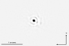 |
Fig. 1 Diffraction-limited image of HD 176986 after lucky imaging processing with a selection of the 10% best individual TCS/FastCam frames. |
3 Determination of stellar activity indicators and radial velocities
3.1 SMW index
We calculated the Mount Wilson S index (SMW) and the  using the original Noyes et al. (1984) procedure, following Lovis et al. (2011) and Suárez Mascareño et al. (2015). We defined two triangular passbands with a full-width at half-maximum (FWHM) of 1.09 Å centred at 3968.470 Å and 3933.664 Å for the Ca II H&K line cores, and for the continuum, we used two20 Å wide bands centred at 3901.070 Å (V ) and 4001.070 Å(R), as shown in Fig. 2.
Then the SMW index is defined as
 (1)
(1)
where ÑH, ÑK, ÑR, and ÑV are the mean fluxes per wavelength interval in each passband, while α and β are calibration constants fixed as α = 1.111 and β = 0.0153. The S index servesas a measurement of the Ca II H&K core flux normalized to the neighbour continuum. As a normalized index to compare it to other stars, we computed the  following Suárez Mascareño et al. (2015).
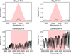 |
Fig. 2 Ca IIH&K filter of the spectrum of the star HD 176986 with the same shape as the Mount Wilson Ca II H&K passband. |
3.2 Hα index
We also used the Hα index, with a simpler passband following Gomes da Silva et al. (2011). It consists of a rectangular bandpass with a width of 1.6 Å and centred at 6562.808 Å (core), and two continuum bands of 10.75 Å and 8.75 Å in width, centred at 6550.87 Å (L) and 6580.31 Å (R), respectively, as shown in Fig. 3.
Thus, the Hα index is defined as
 (2)
(2)
where  and
and  are the mean fluxes per wavelength interval in each passband.
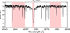 |
Fig. 3 Spectrum of the K-type star HD 176986 showing the Hα filter passband and continuum bands. |
3.3 Radial velocities
The RV measurements in the HARPS and HARPS-N standardpipelines are determined by a Gaussian fit of the cross-correlation function (CCF) of the spectrum with a binary stellar template (Baranne et al. 1996; Pepe et al. 2000).
4 Analysis
Using all the available datasets, we searched for periodic signals that are compatible with planetary companions, stellar rotation, and long-term magnetic cycles. We computed the power spectrum using a least-squares periodogram (Cumming 2004) by fitting a sinusoidal model over the whole range of test frequencies using the MPFIT routine (Markwardt 2009), with the power spectral density (PSD) defined following Zechmeister & Kürster (2009). The significance of the periodogram peaks was evaluated by calculating the spectral density thresholds for the desired false-alarm probability (FAP) levels using bootstrap randomization (Endl et al. 2001) of the data. When we detected a significant signal, we re-computed the periodogram using the superposition of two signals, one with a period fixed at the detected peak of the periodogram, and a new sinusoidal model again evaluated over the whole range of test frequencies. The amplitudes and phases of both signals were set free to ensure the best fit at each test period. We recursively repeated the procedure by adding new signals until no more significant signals were found in the data (Arriagada et al. 2013), with the FAP levels re-calculated at each step.
During this stage, all the signals detected in the recursive periodograms (in all datasets: RV, FWHM, bisector span, SMW index, Hα index, ASAS photometry) were modelled using a double-harmonicsinusoidal model (Berdyugina & Järvinen 2005) with the IDL MPFIT routine (Markwardt 2009). This model easily allows accounting for the asymmetry that is expected for activity signals and also maintains a sinusoidal shape for sinusoidal signals. When the origin of the signals was established, RV planetary signals were modelled using Keplerian models, whose parameters were calculated by performing a Bayesian analysis, using the Markov chain Monte Carlo (MCMC) code built in The Data & Analysis Center for Exoplanets (DACE)3.
4.1 Stitching HARPS and HARPS-N data together
HARPS and HARPS-N are almost identical spectrographs, but this does not mean that their data can be combined as if they were the same instrument. The HARPS set of fibres was upgraded during May 2015, which also means that HARPS post-upgrade data need to be analysed as data from a different instrument. The offets between the data coming from both instruments are not large, but still need to be estimated. The offsets between the different datasets were estimated as free parameters in the fits, using the HARPS pre-upgrade dataset as reference. Table 2 shows the offsets applied to the HARPS post-upgrade and HARPS-N data. The offsets estimated between the different datasets are consistent with previous measurements for similar stars (Desidera et al. 2013; Lo Curto et al. 2015).
Offsets applied.
4.2 Analysis of the radial velocity variability
Our RV dataset consists of 259 RV measurements distributed along 13.2 years with a good coverage of almost the whole baseline. We measured a mean RV of the star of 37.74 km s−1, an RMS of the measurements of 3.8 m s−1 , and a typical uncertainty of 1.0 m s−1 per individual measurement, including photon noise, pointing errors, and drift measurement errors. Figure 4 shows the available RV dataset.
By calculating the recursive periodograms and identifying the most significant signals at every iteration, we detected three dominant signals in the RV data. The three identified peaks in the periodograms correspond to a 16.82 ± 0.01 d signal with a semi-amplitude of 2.59 ± 0.36 m s−1 , a 6.49 ± 0.01 d signal with a semi-amplitude of 2.37 ± 0.35 m s−1 , and a 35.74 ± 0.02 d signal with a semi-amplitude of 1.20 ± 0.35 m s−1 . The three signals are detected with FAPs several orders of magnitude smaller than 0.1%. The signals detected at 16.82 and 6.49 d are consistent with sinusoidals, while the signal at 35.74 d is highly non-sinusoidal. The amplitude ratios between the sinusoidal signals at P/2 and the sinusoidal signals at P are smaller than the 0.1 for the signals at 16.82 and 6.49 d, while for the case of the 35.74 d, the ratio is 0.6. The 35.7 d signal is consistent with previous measurements of the rotation period of the star (Suárez Mascareño et al. 2015, 2017c), while the signal at 16.82 days is one day apart from the first harmonic of that measurement of stellar rotation. Figure 5 shows the recursive periodograms of the RV time-series; the three signals are highlighted. Figure 6 shows the phase-folded fits to the data after removing the contributions of all the other signals.
We did not find more significant signals in the RV data. The RMS of the residuals after fitting the three signals is approximately 2.5 m s−1 . Given the small uncertainty of the individual measurements, there is still room for more signals that we do not detect. These hypothetical signals could be of very low amplitude, especially if the periods are long. Another possibility is that the scatter is caused by undetected quasi-periodic signals or activity signals that may not be stable in time.
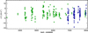 |
Fig. 4 Radial velocity time-series for the star HD 176986 obtained by combining HARPS and HARPS-N measurements. Green filled dots show HARPS pre-upgrade data, green empty dots show HARPS post-upgrade data, and blue filled dots show HARPS-N data. |
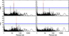 |
Fig. 5 Periodograms of the RV time-series. The shaded region highlights the detected periodicities of 16.83 d (top left), 6.49 d (top right), and 35.74 d (bottom left). The red dotted, green dashed, and blue solid horizontal lines show the 10%, 1%, and 0.1% FAP levels. |
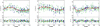 |
Fig. 6 Phase-folded curve of the RV time-series using the 16.82 d signal (left panel), the 6.49 d signal (centre panel), and the 35.74 d signal (right panel). Green filled dots show HARPS pre-upgrade data, green empty dots show HARPS post-upgrade data, and blue filled dots show HARPS-N data. Red empty dots are the same points binned in phase with a bin size of 0.1. The error bar of a given bin is estimated using the weighted standard deviation of the binned measurements divided by the square root of the number of measurements included in this bin. The dark red line shows the best fit to the data using double sinusoidals at P and P/2 for all the signals. In each case, the contribution of the other two detected signals has been subtracted. |
4.3 Analysis of the FWHM variability
The FWHMmeasurements show a mean measurement of 6.13 km s−1 with an RMS of the measurements of 12.5 m s−1 and a typical uncertainty of the measurements of 3.7 m s−1 (see Fig. 7).
The periodogram FWHM time-series show a single significant signal at the period of 36 days (see Fig. 8). Using a double-sinusoidal fit, we measure a period of 36.00 ± 0.03 days and a semi-amplitude of 6.6 ± 1.4 m s−1 (see Fig. 9). The phase-folded fit is highly non-sinusoidal, very similar to the 35.7-day signal found in the RV dataset. The signal is consistent with the expected rotation period of a main-sequence K-dwarf of this activity level and with previous measurements that used a subset of the same data (Suárez Mascareño et al. 2015). No more significant signals are found after subtracting the 36-day signal.
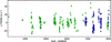 |
Fig. 7 Time-series for FWHM variations of the star HD 176986, obtained by combining HARPS and HARPS-N data. See Fig. 4 for reference. |
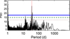 |
Fig. 8 GLS periodogram of the variations of the FWHM time-series. The shaded region shows the detected periodicity of 36 d. |
4.4 Analysis of the bisector span variability
For the bisector span, we have a mean measurement of 14.82 m s−1 with an RMS of the measurements of 2.8 m s−1 and a typical uncertainty of 1.8 m s−1, using Boisseet al. (2009) as a reference (see Fig. 10). The periodogram shows two significant signals at 1670 ± 29 days and 19.20 ± 0.01 days (Fig. 11) with semi-amplitudes of 1.41 ± 0.39 m s−1 and 1.22 ± 0.30 m s−1 . Figure 12 shows the best fits to both signals using a double-sinusoidal model. The signal is approximately one day apart from the first harmonic of the rotation period of the star. Wedid not find any more significant signals in the residuals of the bisector span data. The scarcity of points at phase 0.6–0.7 in the long-period signal leaves some doubts about its true nature. It is possible that it is mostly a window effect.
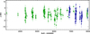 |
Fig. 10 Time-series for variations of the bisector span of the CCF ofthe star HD 176986, obtained by combining HARPS andHARPS-N data. See Fig. 4 for reference. |
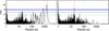 |
Fig. 11 GLSperiodogram of the variations of the bisector span time-series. The shaded region shows the detected periodicitiesat 1800 days (left panel) and 19 days (right panel). |
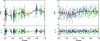 |
Fig. 12 Phase-folded curve of the bisector span time-series using the 1670-day signal (left panel) and the 19.2-day signal (right panel). See Fig. 6 for reference. |
4.5 Analysis of the Ca II H & K variability
We measured a mean SMW value of 0.2916 with an RMS of the measurements of 0.0165 and a typical uncertainty of 0.0053 per exposure (see Fig. 13). A long-period signal is clearly visible in the time-series, with a length consistent with a solar-like magnetic cycle. The periodogram shows two dominant signals in the data (Fig. 14) at 2100 days and 36 days. Some other apparently significant signals are visible, but all the long-period signals disappeared when we fitted the long-term signal, and the short-period signal disappeared when we fitted the 36 d signal.
The combined fit of both signals, using double sinusoidals at periods P and P/2, returns a period of 5.67 ± 0.11 yr with a semi-amplitude of 0.0153 ± 0.0018 for the long-period signal and a period of 36.02 ± 0.02 days with a semi-amplitude of 0.0068 ± 0.0016 for the short-period signal. These measurements are consistent with the solar-like cycle and the rotation period of the star, as is also supported by the FWHM and BIS analysis. Figure 15 shows the individual fits of the two signals. They are clearly not sinusoidal, as it is often the case for activity-induced signals.
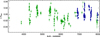 |
Fig. 13 SMW index time series for the star HD 176986, obtained by combining HARPS and HARPS-N data. See Fig. 4 for reference. |
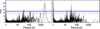 |
Fig. 14 Periodogram for the SMW index time series for the star HD 176986. The shaded region highlights the detected periodicities of 6 yr (left) and 36 days (right). |
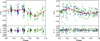 |
Fig. 15 Phase-folded curve of the SMW index time series using the 6.0 yr signal (left panel) and the 36.02 d signal (right panel). See Fig. 6 for reference. |
4.6 Analysis of the Hα variability
For the Hα index, we measured a mean value of 0.228356 with an RMS of the measurements of 0.00108 with a typical uncertainty of the measurements of 0.00032 (see Fig. 16). The periodogram shows two dominant signals at about 2400 and 26 days (Fig. 17). The 26-day signal is more significant than the signal at 2400 days, but inadequate sampling of long-period signals often creates ghost signals in the periodograms when not properly modelled. These ghost signals can sometimes appear to be more significant than the real signals. These ghost signals usually vanish when the long-period signal is fitted and subtracted. We opted to subtract the 2400-day signal before the 26-day signal in order to remove the possible ghost signals that are associated with the 2400-day signal.
The fit of the signals using double sinusoidals at periods P and P/2 returns periods of 8.21 ± 0.24 years and 26.20 ± 0.01 days with a semi-amplitude of 0.00022 ± 0.00013 and 0.00067 ± 0.00011. Figure 18 shows the phase-folded fits to the data.
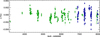 |
Fig. 16 Hα index time-series for the star HD 176986, obtained by combining HARPS and HARPS-N data. See Fig. 4 for reference. |
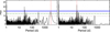 |
Fig. 17 Periodogram for the Hα index time-series for the star HD 176986. The shaded region highlights the detected periodicities of 2400 days (left panel) and 26 days (right panel). |
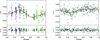 |
Fig. 18 Phase-folded curve of the Hα index time-series using the 2400 d signal (left panel) and the 26 d signal (right panel). See Fig. 6 for reference. |
4.7 Analysis of the photometric variability
The ASAS mV light curve consists of 411 nightly exposures over a baseline of 8.7 years, measuring an average mV of 8.46 with an RMS of 13.4 mmag and a typical uncertainty of the measurements of 10.3 mmag. Figure 19 shows the available light curve. We detected a significant long-period signal at 5.09 ± 0.26 yr with a semi-amplitude of 5.6 ± 1.3 mmag. Figure 20 shows the periodogram and the phase-folded curve. No more significant signals arise after subtracting the long-period signal.
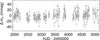 |
Fig. 19 ASAS mV light curve for the star HD 176986. |
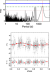 |
Fig. 20 GLS periodogram of the ASAS light curve (top panel). The shaded region shows the periods estimated by the least-squares double-sinusoidal fit. The bottom panel shows the phase-folded curve of the data using the period highlighted in the top panel. Grey dots show the individual measurements after subtracting a long-period linear trend. See Fig. 6 for reference. |
5 Analysis and interpretation of the detected periodicities
The previous analysis unveils several periodic signals ranging from 6 days to 8 years. Some of them are exclusive to a single dataset, while others are common to different data series. We can summarize the detected signals as a 6.5 d signal detected in the RV data; a 16.8 d signal detected in the RV data; a 19 d signal detected in the bisector span data; a 26 d signal detected in the Hα index data; a 36 d signal detected simultaneously in the RV, FWHM, and SMW index data; and a group of signals ranging from 4 to 8 yr detected in the bisector, SMW index , Hα index data and in the mV light curve. Table 3 shows the periods and uncertainties of all the detected signals.
Signals that are simultaneously detected in RV and in one or several of the activity indicators are in most cases induced by stellar activity. Although there is no physical reason why a planet cannot orbit a star with a period equal to the rotation or the magnetic cycle of the star, separating the two signals in order to prove the Keplerian origin of the RV signal is often very difficult. Based on this assumption, we can separate the RV signals into two different groups. One group is probably associated with stellar activity (35.8 d), and the other group might have a Keplerian origin (6.5 d and 16.8 d). Some remaining signals are only present in the activity proxies (19 and 26 d, and three long-period signals).
Given the spectral type of the star (K2.5), its mean level of stellar activity (log10 ( ) = – 4.90) and the previous measurements of Suárez Mascareño et al. (2015, 2017c), which were performed over a much shorter baseline, we expect a rotation period of 37 ± 6 days (Suárez Mascareño et al. 2016). We can safely say that the different signals at around 36 days are all related to the rotation of the star. The amplitude of the RV signal at this period is consistent with the measurement of the activity-induced signal measured in Suárez Mascareño et al. (2017c), even though the measured periods are different (it has to be noted that the period was calculated using a subset of the data used in this work). The 40 d period measured in Suárez Mascareño et al. (2017c) seems to be the 1 yr alias of the real rotation signal.
The 19-day signal present in the bisector span data is very close to half of the rotation period. The combination of the geometrical distribution of active regions and the inclination of the rotation axis of the star can easily create a pattern in which the rotation signal and its first harmonic are super-imposed (Boisse et al. 2011; Dumusque et al. 2011, 2014; Suárez Mascareño et al. 2017c). The highly non-sinusoidal shape of the signals identified at the rotation period (see Figs. 6, 9, and 15) suggests a very inhomogeneous distribution of activity regions that might lead to the detection of signals at the harmonics of the rotation period.
The different long-period signals present both in the bisector, SMW index, Hα index time-series, and in the mV light curve are compatible with a solar-like cycle. The length of that cycle is still not well defined, considering the scatter of the different measurements, but the SMW index measurement is probably the most accurate measurement, as it has the largest amplitude. A longer baseline is needed to completely establish the cycle length, but based on our measurements, we assume that it is close to five years. We did not find a similar signal in the RV data, which supports the conclusions of Santos et al. (2010).
The origin of the 26 d signal in the Hα index might be indicating activity regions that lie closer to the equator than those producing the 36 d signal. The Sun’s differential rotation causes the rotation period to change from 25 days at the equator to 36 days at the poles. We might be seeing a similar behaviour, although this would imply a very extreme scenario. The Hα measurement showing the evolution of equatorial active regions, while every other activity proxy showing the evolution of polar active regions. This seems a rather unlikely scenario. The variations in Hα index for K-type stars are very small and sometimes harder to interpret than in the case of M-dwarfs or the variations in SMW index. Given the low amplitude measured of the variations in Hα index, we cannot rule out that the 26 d signal is not a real signal, but a combination of the 19 d and 36 d signals.
The signals at 6.49 d have no counterpart in the time-series of activity proxies, which favours the interpretation of a Keplerian origin. The 16.82 d signal does not have a direct counterpart in any of the activity proxy time-series, but it lies close to the first harmonic of the rotation signal, which means that we need to be careful when we interpret this signal.
As a test of the origin of the detected signals, we studied the Spearman correlation coefficient between the different time-series and the different individual signals. To measure the correlations between individual signals, we created individual datasets by subtracting all the other contributions, and we isolated the studied signal. The significance of the correlation was evaluated by performing 10 000 bootstrap simulations (Endl et al. 2001). No correlation was found between any of the RV datasets and the bisector or Hα datasets. There is evidence for a weak correlation between the raw RV data and the FWHM and SMW index data. The correlation became non-significant when we tested the datasets that included only the 6.49-day or 16.82-day signals, or both. On the other hand, the correlation increased when we tested the dataset that included the 35.74-day RV signal. To further test this correlation, we fitted and subtracted a linear relationship between the FWHM and the RV data. The resulting dataset shows the 6.49- and 16.82-day signals intact, while the amplitude of the 35.74-day signal decreases significantly. The same test with the SMW index data produced the same effect. This favours the interpretation that the 35.74-day RV signal shares an origin with the 36-day activity signals. We did not find a correlation between any of the datasets that included only the 6.49- and/or 16.82-day signals and any of the activity index time-series. This favours a Keplerian interpretation for the two signals.
Keplerian signals are deterministic and consistent in time. When an individual signal is measured, the significance of the detection is expected to increase steadily with the number of observationsand the measured period is expected to be stable over time. However, in the case of an activity-related signal, this is not necessarily the case. As the stellar surface is not static and the configuration of active regions may change with time, changes in the modulation phase and in the detected period are expected (Affer et al. 2016; Suárez Mascareño et al. 2017a,b; Mortier & Collier Cameron 2017). Even the disappearance of the signal at certain seasons is possible. To study the evolution of the two signals, we performed a simultaneous fit of the detected periodicities in each of the time-series, and then used the derived parameters to subtract thecontribution of one of them, which left the other “isolated”. We then performed the stacked periodograms using a verynarrow frequency window around each of the signals. Figure 21 shows the evolution of the significance of the detection of all the signals after subtracting all the other detected components, against the number of observations and the date of observation. When the signal-to-noise ratio is high enough (after the signal crosses the 1% FAP threshold), the evolution of the 6.5 d and 16.8 d singals is steady and continuous. The slope of the 16.8 d signal is slightly steeper, which is to be expected given its larger amplitude. The behaviour of the 35 d signal, on the other hand, is very erratic. It almost disappears after crossing the 0.1% FAP threshold and recovers later. The result of this test favours the interpretation that the 6.49 d and 16.82 d signals are Keplerian signals and that the 36 d signal is an activity signal. Following the same reasoning as for the previous test, we expect the measured semi-amplitude of planetary signals to converge with the number of observations. Before they become significant, the 6.49 d and 16.82 d signals already show amplitudes that are compatible with the final measurement (see Fig. 22). The amplitude of these signals shows very small variability even before the signals cross the 1% FAP threshold, and slopes that are compatible with flat lines. On the other hand, the 35.74-day signal shows a very steep negative slope and a variability greater than 77% in its final amplitude. The signal amplitude increases significantly after 130 measurements (2014) and then decreases again after 200 measurements (2016). By studying the evolution against the date of observations, we can also see the importance of the high-cadence observation campaigns. The slope of the significance is greatly increased after the start of the HARPS-N nightly cadence campaigns, which means that the time needed for the detection of short-period planets decreases significantly, similar to what happened with the discovery of Proxima b (Anglada-Escudé et al. 2016).
Finally, an analysis of the spectral window ruled out that the peaks in the periodogram are artefacts of the time sampling alone. Following Rajpaul et al. (2016), we checked that no features appeared at 6.5, 16.8, or 35.7 days even after masking the oversaturated regions of the power spectrum. We then tried to re-create the planet candidate signals by injecting the detected signals corresponding to PRot and PRot/2 along with a low-amplitude signal (<1 m s−1 ) at the period of the magnetic cycle (6 yr). We performed 10 000 simulations with randomized periods and amplitudes (compatible with the measured uncertainties) and randomized phase shifts along with a white-noise model with an RMS of 1.9 m s−1 . Figure 23 shows the results of these simulations; the periods attributed to the planetary candidates are highlighted. We were never able to generate the signals at 6.5 or 16.8. It seems very unlikely that any of the candidate planetary signals are artefacts of the sampling or ghost signals created by the combination of activity signals. This test also shows that for future studies of this star, it is important to be very careful with periodicities that are detected between 25 and 45 days, as the combination of the different activity signals detected might generate several artefacts in that range. It is also important to note that it seems possible to generate a 26-day peak in the periodogram by combining the 35.7 d signal and a signal at half that period with the appropriate phase difference and amplitude, which might explain the 26-day signal in the Hα index time-series that does not appear in any other time-series.
After these tests, we conclude that the signals at 6.5 days and 16.8 days are of Keplerian origin, while the signal at 35.8 days is of stellar origin.
Summary of the detected signals in the different datasets of HD 176986.
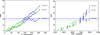 |
Fig. 21 Evolution of the significance of the detected signals as a function of the number of measurements (left panel) andthe date of the observations (right panel). Green filleddots, green empty dots, and blue filled dots show the HARPS pre-upgrade, HARPS post-upgrade, and HARPS-N measurements, respectively. The horizontal red dotted line, green dashed line, and blue solid line show the 10%, 1%, and 0.1% FAP thresholds. The grey dashed lines show a linear fit to the evolution of the PSD after the signals cross the 1% FAP threshold. |
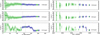 |
Fig. 22 Evolution of the measured semi-amplitude of every detected signal as a function of the number of measurements (left panel) and the date of the observations (right panel), using a double-sinusoidal model as in Sect. 4.2. Green filled dots, green empty dots, and blue filled dots show the HARPS pre-upgrade, HARPS post-upgrade, and HARPS-N measurements, respectively. The vertical black dashed line shows the moment at which each signal crosses the 1% FAP threshold. The grey dashed lines show a linear fit to the evolution of the PSD after the signals cross the 1% FAP threshold. |
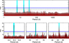 |
Fig. 23 Periodogram of the synthetic data created by injecting the 35.7 d signal, along with a low-amplitude 6 yr signal and a white-noise model. The black line shows the real RV periodogram. The dark red, red, and light red regions show the PSD level that is reached at every individual frequency at least in 10%, 1%, and 0.1% of the simulations. The vertical light blue lines show the position of the detected RV signals. The bottom panels are zoom-ins around the regions of the three detected RV signals. The black line in this case shows the RV periodogram after subtracting the contributions of all the other signals. |
6 The planetary system of HD 176986
The analysis of the RV time-series and of the activity indicators leads us to conclude that the best explanation of the observed data is that two planets orbit the star HD 176986. TheRV series also shows two different activity signals that are related to the stellar rotation and its first harmonic.
In orderto calculate the final parameters and quantify the uncertainties of the orbital parameters of the planets, we performed a Bayesian analysis using the MCMC code built in the DACE platform, which is described in Díaz et al. (2014, 2016). We fitted an RV model composed of three Keplerians; we decided to model the activity signals as Keplerians. The MCMC analysis was performed with uniform priors for all variables, with the exception of the stellar mass, for which a Gaussian prior was used. To take the uncertainties due to instrumental systematics and stellar signals not estimated during the analysis process into account, we included in the MCMC analysis a white-noise jitter parameter that was added quadratically to the individual RV error bars.
Figure 24 shows the posterior distribution of the parameters of the planetary system, and in Table 4 we show the final parameters and uncertainties obtained with the Bayesian MCMC analysis. It is important to note that the obtained amplitude for the stellar-induced RV signal is very different from the amplitude measured in previous sections. This is a side effect of using a Keplerian to model the signal instead of the double-sinusoidal model.
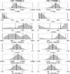 |
Fig. 24 Posterior distribution of the model parameters of the planetary companions of the K dwarf star HD 176986. The vertical dashed line shows the median value of the distribution, and the dotted lines represent the 1σ values. |
Parameters of the HD 176986 planetary system.
6.1 Gaussian processes analysis
Gaussian processes (GP) are becoming increasingly common in the analysis of stellar activity in RV time-series. Here we treated the stellar activity term as correlated quasi-periodic noise, using the approach based on GPs (see Rasmussen & Williams (2006) and Robertset al. (2012)). The stellar noise is described by a covariance functional form, and the parameters have some correspondence to the physical phenomena to be modelled. The GP framework can be used to characterize the activity signal without requiring a detailed knowledge of the distribution of active regions on the stellar surface, their lifetimes, or their temperature contrast.
To model the short-term activity, we used the publicly available GEORGE Python library for GP regression (Ambikasaran et al. 2014), and adopted the quasi-periodic kernel described by the covariance matrix
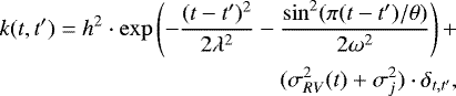 (3)
(3)
where t and t′ indicate two different epochs. This kernel has been widely used with great success in recent exoplanet publications (Haywood et al. 2014; Faria et al. 2016; Affer et al. 2016), as its functional form encompasses some known properties of stellar activity. It is composed of a periodic term coupled to an exponential decay term, and the kernel describes a recurrent signal linked to the stellar rotation and takes the finite lifetime of the active regions and evolution of their size into account. The parameters h in the covariance function represent the amplitude of the correlations, θ is the rotation period of the star, ω is the amplitude scale of the periodic component (linked to the evolution in size of active regions), and λ is the correlation decay timescale (related to the lifetime of the active regions). The equation also includes a term of uncorrelated noise, added quadratically to the diagonal of the covariance matrix.  is the RV uncertainty at time t, and
  is the additional noise fit in the model to take other noise sources into account that are not included in the internal errors and in the stellar activity framework.
For the parameters of the covariance kernel, we assigned log-uniform priors in sensible ranges. For θ, the parameter that can be interpreted as the stellar rotation period, we have several previous measurements that place it at 36 days. Table 5 shows the parameters obtained through the GP analysis and the priors used for each parameter. The GP parameters for the two Keplerian signals are consistent with those obtained with the MCMC analysis. The GP MCMC converged towards the previously measured periods. For the case of the activity signal, the measurement of the rotation period coincides with our previous measurements, and the decay timescale also seems to be consistent with what is expected for a main-sequence star (Giles et al. 2017).
Parameters of the HD 176986 planetary system given by the Gaussian processes analysis.
6.2 Dynamical analysis
The two HD 176986 planets are very close to each other. Planet-planet interactions might occur when planets oribt so closely to each other, especially somewhat massive planets, which mightlead to unstable configurations. A necessary step when analysing a system like this is to test for its long-term stability. We tested the stability of the whole system using the DACE built-in implementation of the GENGA N-body simulations code (Grimm & Stadel 2014). The global analysis shows the system to be stable over scales of giga years, and shows the semi-major axis and eccentricities of the planets to be very stable along the whole simulation, and the peak-to-peak variation of the eccentricities is smaller than 10−5 and 10−4 for planets b and c, respectively.
To test the regions of the parameter space where the system might be stable, we then built stability maps for each of the two planets. For each planet, the system was integrated on a regular 2D mesh of initial conditions, with varying semi-major axis and eccentricity, while the other parameters were kept at their estimated values. For each initial condition, the system was integrated over 104 yr and a stability criterion was derived with the frequency analysis of the mean longitude (Laskar 1990, 1993). In all cases, the 1σ confidence interval is fully compatibly with regions where the system would be stable for timescales comparable with or much longer than the age of the system.
7 Discussion
We detected a system of two planets with semi-amplitudes of 2.56 m s−1 and 2.63 m s−1 . Based on the stellar mass of 0.789 M⊙, this is converted into mp sini of 5.74 M⊕ and 9.18 M⊕, and the planets orbit with periods of 6.49 d and 16.82 d around HD 176986, a K2.5-type star with a mean rotation period of about 36 days and a 6 yr activity cycle. The two planets would be at orbital distances of 0.063 AU and 0.119 AU. Following Queloz et al. (1998); Weise et al. (2010), we estimated the v sin i to be 1.10 ± 0.20 km s−1 , which means a P sin i of 36 ± 4 days. This means that the rotation axis of the star is compatible with an edge-on configuration. If the orbital and rotation axis were aligned, this would mean that our estimation for the minimum masses would be very close to the true masses of the planets, and would make the star a very interesting candidate for a transit follow-up.
The two detected planets may be super-Earths, and HD 176986 c has a greater chance of being a mini-Neptune. The two planets are too close to their host star to be considered habitable. For the two planets HD 176986 b and c, we measured an effective flux of 83.5 ± 6.9 and 23.5 ± 4.5 times the flux received by Earth, rendering all of them most likely inhabitable, independently of the planetary conditions. Table 6 shows the limits of the habitable zone of HD 176986 for a variety of scenarios.
HD 176986 is a quiet early K-dwarf, with a rotation period of 36 days, which is a typical rotation period for a quiet star of its kind (Suárez Mascareño et al. 2016). Its rotation-induced RV signal has a semi-amplitude of 1.2 ms−1 (double sinusoidal), 2.9 ms−1 (Keplerian), or 3.1 ms−1 (GP), depending on the model used; this signal does not remain stable with time. The double-sinusoidal model gives the smallest amplitude, and the GP analysis gives the largest amplitude. We find a second activity signal at 19 days that is probably related to the first harmonic of the rotation period and that only appears in the bisector span time-series. The star exhibits a 6 yr magnetic cycle for which we did not detect any measurable induced RV signal, supporting the conclusions of Santoset al. (2010).
Given the rms of the residuals of the LS-fit or the MCMC, there is still room for the detection of more planets in this system. These hypothetical planets, if present, should be smaller than 6 MEarth for periods shorter than 180 days. For the periods corresponding to the conservative habitable zone, planets of up to 10 MEarth could have been undetected. The region between 20–50 days would be difficult to explore. The rotation signal and the artefacts it creates strongly contaminate the periodogram from ~20 to at least ~50 days. Between ~50 to ~100 days, a possible planet should be smaller than 4 MEarth to not appear even as a candidate signal in our data. The GP analysis, on the other hand, leaves a smaller room for additional planets. There could still be very low-mass planets in the system, but the probability of finding them seems rather low.
Limits of the habitable zone for HD 176986.
8 Conclusions
We have analysed 250 high-resolution spectra taken with HARPS and HARPS-N along with photometric observations in V band to study the planetary companions around the K-dwarf star HD 176986 and its stellar activity. We detected the presence of three significant RV signals.
We conclude that two signals at periods of 6.49 d and 16.82 d are caused by two planets with minimum masses of 5.74 M⊕ and 9.18 M⊕ in orbits with semi-major axes of 0.063 AU and 0.119 AU. Our estimation of the v sin i makes the system compatible with an edge-on configuration, which means that the true masses of the planets might be very close to the minimum masses; the system is a very promising candidate for a transit follow-up.
The remaining signal is the rotation-induced RV signal at 36 days. The measured rotation period and the amplitude of the rotation-induced signal match the expected results of Suárez Mascareño et al. (2015, 2016, 2017c). We also found evidence for a magnetic cycle of ~6 yr, which needs future observations to be better constrained.
We performed a dynamical analysis of the system and found it to be stable over long periods of time, comparable to the age of the system.
Acknowledgements
A.S.M acknowledges financial support from the Swiss National Science Foundation (SNSF). This work has been partially financed by the Spanish Ministry project MINECO AYA2014-56359-P. J.I.G.H. acknowledges financial support from the Spanish MINECO under the 2013 Ramón y Cajal program MINECO RYC-2013-14875. PF and NCS acknowledge support by Fundação para a Ciência e a Tecnologia (FCT) through Investigador FCT contracts of reference IF/01037/2013/CP1191/CT0001 and IF/00169/2012/CP0150/CT0002, respectively, and POPH/FSE (EC) by FEDER funding through the program “Programa Operacional de Factores de Competitividade – COMPETE”. PF further acknowledges support from Fundação para a Ciência e a Tecnologia (FCT) in the form of an exploratory project of reference IF/01037/2013/CP1191/CT0001. This work is based on data obtained via the HARPS public database at the European Southern Observatory (ESO). This research has made extensive use of the SIMBAD database, operated at CDS, Strasbourg, France, and NASA’s Astrophysics Data System. This publication makes use of The Data & Analysis Center for Exoplanets (DACE), which is a facility based at the University of Geneva (CH) dedicated to extrasolar planets data visualisation, exchange and analysis. DACE is a platform of the Swiss National Centre of Competence in Research (NCCR) PlanetS, federating the Swiss expertise in Exoplanet research. The DACE platform is available at https://dace.unige.ch.
References
- Affer, L., Micela, G., Damasso, M., et al. 2016, A&A, 593, A117 [NASA ADS] [CrossRef] [EDP Sciences] [Google Scholar]
- Ambikasaran, S., Foreman-Mackey, D., Greengard, L., Hogg, D. W., & O’Neil, M. 2014, IEEE Trans. Pattern Anal. Mach. Intell., 38, 2 [Google Scholar]
- Anglada-Escudé, G., Amado, P. J., Barnes, J., et al. 2016, Nature, 536, 437 [NASA ADS] [CrossRef] [PubMed] [Google Scholar]
- Arriagada, P., Anglada-Escudé, G., Butler, R. P., et al. 2013, ApJ, 771, 42 [NASA ADS] [CrossRef] [Google Scholar]
- Astudillo-Defru, N., Forveille, T., Bonfils, X., et al. 2017, A&A, 602, A88 [NASA ADS] [CrossRef] [EDP Sciences] [Google Scholar]
- Baranne, A., Queloz, D., Mayor, M., et al. 1996, A&AS, 119, 373 [NASA ADS] [CrossRef] [EDP Sciences] [Google Scholar]
- Benz, W., Ida, S., Alibert, Y., Lin, D., & Mordasini, C. 2014, in Protostars and Planets VI (Tucson: University of Arizona Press), 691 [NASA ADS] [Google Scholar]
- Berdyugina, S. V. & Järvinen, S. P., 2005, Astron. Nachr., 326, 283 [NASA ADS] [CrossRef] [Google Scholar]
- Boisse, I., Moutou, C., Vidal-Madjar, A., et al. 2009, A&A, 495, 959 [NASA ADS] [CrossRef] [EDP Sciences] [Google Scholar]
- Boisse, I., Bouchy, F., Hébrard, G., et al. 2011, A&A, 528, A4 [NASA ADS] [CrossRef] [EDP Sciences] [Google Scholar]
- Borucki, W. J., Koch, D. G., Basri, G., et al. 2011, ApJ, 736, 19 [NASA ADS] [CrossRef] [Google Scholar]
- Boyajian, T. S., von Braun, K., van Belle, G., et al. 2012, ApJ, 757, 112 [NASA ADS] [CrossRef] [Google Scholar]
- Cosentino, R., Lovis, C., Pepe, F., et al. 2012, in Ground-based and Airborne Instrumentation for Astronomy IV, Proc. SPIE, 8446, 84461V [CrossRef] [Google Scholar]
- Cumming, A. 2004, MNRAS, 354, 1165 [NASA ADS] [CrossRef] [Google Scholar]
- Desidera, S., Sozzetti, A., Bonomo, A. S., et al. 2013, A&A, 554, A29 [NASA ADS] [CrossRef] [EDP Sciences] [Google Scholar]
- Díaz, R. F., Almenara, J. M., Santerne, A., et al. 2014, MNRAS, 441, 983 [NASA ADS] [CrossRef] [Google Scholar]
- Díaz, R. F., Ségransan, D., Udry, S., et al. 2016, A&A, 585, A134 [NASA ADS] [CrossRef] [EDP Sciences] [Google Scholar]
- Dumusque, X., Santos, N. C., Udry, S., Lovis, C., & Bonfils, X. 2011, A&A, 527, A82 [NASA ADS] [CrossRef] [EDP Sciences] [Google Scholar]
- Dumusque, X., Pepe, F., Lovis, C., et al. 2012, Nature, 491, 207 [NASA ADS] [CrossRef] [PubMed] [Google Scholar]
- Dumusque, X., Boisse, I., & Santos, N. C. 2014, ApJ, 796, 132 [NASA ADS] [CrossRef] [Google Scholar]
- Endl, M., Kürster, M., Els, S., Hatzes, A. P., & Cochran, W. D. 2001, A&A, 374, 675 [Google Scholar]
- Faria, J. P., Haywood, R. D., Brewer, B. J., et al. 2016, A&A, 588, A31 [NASA ADS] [CrossRef] [EDP Sciences] [Google Scholar]
- Fressin, F., Torres, G., Charbonneau, D., et al. 2013, ApJ, 766, 81 [NASA ADS] [CrossRef] [Google Scholar]
- Gaia Collaboration (Brown, A. G. A., et al.) 2016, A&A, 595, A2 [NASA ADS] [CrossRef] [EDP Sciences] [Google Scholar]
- Giles, H. A. C., Collier Cameron, A., & Haywood, R. D. 2017, MNRAS, 472, 1618 [Google Scholar]
- Gillon, M., Triaud, A. H. M. J., Demory, B.-O., et al. 2017, Nature, 542, 456 [NASA ADS] [CrossRef] [PubMed] [Google Scholar]
- Gomes da Silva, J., Santos, N. C., Bonfils, X., et al. 2011, A&A, 534, A30 [NASA ADS] [CrossRef] [EDP Sciences] [Google Scholar]
- Gray, R. O., Corbally, C. J., Garrison, R. F., et al. 2006, AJ, 132, 161 [NASA ADS] [CrossRef] [Google Scholar]
- Grimm, S. L., & Stadel, J. G. 2014, ApJ, 796, 23 [NASA ADS] [CrossRef] [Google Scholar]
- Hatzes, A. P. 2013, ApJ, 770, 133 [NASA ADS] [CrossRef] [Google Scholar]
- Haywood, R. D., Collier Cameron, A., Queloz, D., et al. 2014, MNRAS, 443, 2517 [NASA ADS] [CrossRef] [Google Scholar]
- H∅g, E., Fabricius, C., Makarov, V. V., et al. 2000, A&A, 355, L27 [NASA ADS] [Google Scholar]
- Howard, A. W., Marcy, G. W., Johnson, J. A., et al. 2010, Science, 330, 653 [NASA ADS] [CrossRef] [PubMed] [Google Scholar]
- Huélamo, N., Figueira, P., Bonfils, X., et al. 2008, A&A, 489, L9 [Google Scholar]
- Kopparapu, R. K. 2013, ApJ, 767, L8 [NASA ADS] [CrossRef] [Google Scholar]
- Labadie, L., Rebolo, R., Villó, I., et al. 2011, A&A, 526, A144 [NASA ADS] [CrossRef] [EDP Sciences] [Google Scholar]
- Laskar, J. 1990, Icarus, 88, 266 [NASA ADS] [CrossRef] [Google Scholar]
- Laskar, J. 1993, Physica D Nonlinear Phenomena, 67, 257 [Google Scholar]
- Lo Curto, G., Pepe, F., Avila, G., et al. 2015, The Messenger, 162, 9 [NASA ADS] [Google Scholar]
- Lovis, C., Ségransan, D., Mayor, M., et al. 2011, A&A, 528, A112 [NASA ADS] [CrossRef] [EDP Sciences] [Google Scholar]
- Markwardt, C. B. 2009, in Astronomical Data Analysis Software and Systems XVIII, eds. D. A. Bohlender, D. Durand, & P. Dowler, ASP Conf. Ser., 411, 251 [NASA ADS] [Google Scholar]
- Mayor, M., Pepe, F., Queloz, D., et al. 2003, The Messenger, 114, 20 [NASA ADS] [Google Scholar]
- Mayor, M., Bonfils, X., Forveille, T., et al. 2009, A&A, 507, 487 [Google Scholar]
- Mayor, M., Marmier, M., Lovis, C., et al. 2011, ArXiv e-prints [arXiv:1109.2497] [Google Scholar]
- Mayor, M., Lovis, C., & Santos, N. C. 2014, Nature, 513, 328 [NASA ADS] [CrossRef] [PubMed] [Google Scholar]
- Mordasini, C., Alibert, Y., Klahr, H., & Henning, T. 2012, A&A, 547, A111 [NASA ADS] [CrossRef] [EDP Sciences] [Google Scholar]
- Mortier, A. & Collier Cameron, A. 2017, A&A, 601, A110 [NASA ADS] [CrossRef] [EDP Sciences] [Google Scholar]
- Noyes, R. W., Hartmann, L. W., Baliunas, S. L., Duncan, D. K., & Vaughan, A. H. 1984, ApJ, 279, 763 [NASA ADS] [CrossRef] [Google Scholar]
- Oscoz, A., Rebolo, R., López, R., et al. 2008, in Ground-based and Airborne Instrumentation for Astronomy II, Proc. SPIE, 7014, 701447 [CrossRef] [Google Scholar]
- Pepe, F., Mayor, M., Delabre, B., et al. 2000, in Optical and IR Telescope Instrumentation and Detectors, eds. M. Iye & A. F. Moorwood, SPIE, 4008, 582 [NASA ADS] [CrossRef] [Google Scholar]
- Pepe, F., Lovis, C., Ségransan, D., et al. 2011, A&A, 534, A58 [NASA ADS] [CrossRef] [EDP Sciences] [Google Scholar]
- Pepe, F., Cristiani, S., Rebolo, R., et al. 2013, The Messenger, 153, 6 [NASA ADS] [Google Scholar]
- Pojmanski, G. 1997, Acta Astron., 47, 467 [NASA ADS] [Google Scholar]
- Pont, F., Aigrain, S., & Zucker, S. 2011, MNRAS, 411, 1953 [NASA ADS] [CrossRef] [Google Scholar]
- Queloz, D., Allain, S., Mermilliod, J.-C., Bouvier, J., & Mayor, M. 1998, A&A, 335, 183 [NASA ADS] [Google Scholar]
- Rajpaul, V., Aigrain, S., & Roberts, S. 2016, MNRAS, 456, L6 [NASA ADS] [CrossRef] [Google Scholar]
- Rasmussen, C. E. & Williams, C. K. I. 2006, Gaussian Processes for Machine Learning (The MIT Press) [Google Scholar]
- Roberts, S., Osborne, M., Ebden, M., et al. 2012, Phil. Trans. R. Soc. London Ser. A, 371, 20110550 [Google Scholar]
- Robertson, P., Mahadevan, S., Endl, M., & Roy, A. 2014, Science, 345, 440 [NASA ADS] [CrossRef] [Google Scholar]
- Saar, S. H. & Donahue, R. A. 1997, ApJ, 485, 319 [NASA ADS] [CrossRef] [Google Scholar]
- Santos, N. C., Gomes da Silva, J., Lovis, C., & Melo, C. 2010, A&A, 511, A54 [NASA ADS] [CrossRef] [EDP Sciences] [Google Scholar]
- Santos, N. C., Mortier, A., Faria, J. P., et al. 2014, A&A, 566, A35 [Google Scholar]
- Sousa, S. G., Santos, N. C., Mayor, M., et al. 2008, A&A, 487, 373 [NASA ADS] [CrossRef] [EDP Sciences] [MathSciNet] [Google Scholar]
- Suárez Mascareño, A., Rebolo, R., González Hernández, J. I., & Esposito, M. 2015, MNRAS, 452, 2745 [NASA ADS] [CrossRef] [Google Scholar]
- Suárez Mascareño, A., Rebolo, R., & González Hernández, J. I. 2016, A&A,595, A12 [NASA ADS] [CrossRef] [EDP Sciences] [Google Scholar]
- Suárez Mascareño, A., González Hernández, J. I., Rebolo, R., et al. 2017a, A&A, 597, A108 [NASA ADS] [CrossRef] [EDP Sciences] [Google Scholar]
- Suárez Mascareño, A., González Hernández, J. I., et al. 2017b, A&A, 605, A92 [NASA ADS] [CrossRef] [EDP Sciences] [Google Scholar]
- Suárez Mascareño, A., Rebolo, R., González Hernández, J. I., & Esposito, M. 2017c, MNRAS, 468, 4772 [CrossRef] [Google Scholar]
- Tsantaki, M., Sousa, S. G., Adibekyan, V. Z., et al. 2013, A&A, 555, A150 [NASA ADS] [CrossRef] [EDP Sciences] [Google Scholar]
- Udry, S., Mayor, M., Naef, D., et al. 2000, A&A, 356, 590 [NASA ADS] [Google Scholar]
- van Leeuwen, F. 2007, A&A, 474, 653 [Google Scholar]
- Velasco, S., Rebolo, R., Oscoz, A., et al. 2016, MNRAS, 460, 3519 [NASA ADS] [CrossRef] [Google Scholar]
- Weise, P., Launhardt, R., Setiawan, J., & Henning, T. 2010, A&A, 517, A88 [NASA ADS] [CrossRef] [EDP Sciences] [Google Scholar]
- Zechmeister, M. & Kürster, M. 2009, A&A, 496, 577 [Google Scholar]
- Zsom, A., Seager, S., de Wit, J., & Stamenković, V. 2013, ApJ, 778, 109 [NASA ADS] [CrossRef] [Google Scholar]
All Tables
Parameters of the HD 176986 planetary system given by the Gaussian processes analysis.
All Figures
|
Fig. 1 Diffraction-limited image of HD 176986 after lucky imaging processing with a selection of the 10% best individual TCS/FastCam frames. |
| In the text | |
|
Fig. 2 Ca IIH&K filter of the spectrum of the star HD 176986 with the same shape as the Mount Wilson Ca II H&K passband. |
| In the text | |
|
Fig. 3 Spectrum of the K-type star HD 176986 showing the Hα filter passband and continuum bands. |
| In the text | |
|
Fig. 4 Radial velocity time-series for the star HD 176986 obtained by combining HARPS and HARPS-N measurements. Green filled dots show HARPS pre-upgrade data, green empty dots show HARPS post-upgrade data, and blue filled dots show HARPS-N data. |
| In the text | |
|
Fig. 5 Periodograms of the RV time-series. The shaded region highlights the detected periodicities of 16.83 d (top left), 6.49 d (top right), and 35.74 d (bottom left). The red dotted, green dashed, and blue solid horizontal lines show the 10%, 1%, and 0.1% FAP levels. |
| In the text | |
|
Fig. 6 Phase-folded curve of the RV time-series using the 16.82 d signal (left panel), the 6.49 d signal (centre panel), and the 35.74 d signal (right panel). Green filled dots show HARPS pre-upgrade data, green empty dots show HARPS post-upgrade data, and blue filled dots show HARPS-N data. Red empty dots are the same points binned in phase with a bin size of 0.1. The error bar of a given bin is estimated using the weighted standard deviation of the binned measurements divided by the square root of the number of measurements included in this bin. The dark red line shows the best fit to the data using double sinusoidals at P and P/2 for all the signals. In each case, the contribution of the other two detected signals has been subtracted. |
| In the text | |
|
Fig. 7 Time-series for FWHM variations of the star HD 176986, obtained by combining HARPS and HARPS-N data. See Fig. 4 for reference. |
| In the text | |
|
Fig. 8 GLS periodogram of the variations of the FWHM time-series. The shaded region shows the detected periodicity of 36 d. |
| In the text | |
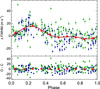 |
Fig. 9 Phase-folded curve of the FWHM time-series using the 36-day signal. See Fig. 6 for reference. |
| In the text | |
|
Fig. 10 Time-series for variations of the bisector span of the CCF ofthe star HD 176986, obtained by combining HARPS andHARPS-N data. See Fig. 4 for reference. |
| In the text | |
|
Fig. 11 GLSperiodogram of the variations of the bisector span time-series. The shaded region shows the detected periodicitiesat 1800 days (left panel) and 19 days (right panel). |
| In the text | |
|
Fig. 12 Phase-folded curve of the bisector span time-series using the 1670-day signal (left panel) and the 19.2-day signal (right panel). See Fig. 6 for reference. |
| In the text | |
|
Fig. 13 SMW index time series for the star HD 176986, obtained by combining HARPS and HARPS-N data. See Fig. 4 for reference. |
| In the text | |
|
Fig. 14 Periodogram for the SMW index time series for the star HD 176986. The shaded region highlights the detected periodicities of 6 yr (left) and 36 days (right). |
| In the text | |
|
Fig. 15 Phase-folded curve of the SMW index time series using the 6.0 yr signal (left panel) and the 36.02 d signal (right panel). See Fig. 6 for reference. |
| In the text | |
|
Fig. 16 Hα index time-series for the star HD 176986, obtained by combining HARPS and HARPS-N data. See Fig. 4 for reference. |
| In the text | |
|
Fig. 17 Periodogram for the Hα index time-series for the star HD 176986. The shaded region highlights the detected periodicities of 2400 days (left panel) and 26 days (right panel). |
| In the text | |
|
Fig. 18 Phase-folded curve of the Hα index time-series using the 2400 d signal (left panel) and the 26 d signal (right panel). See Fig. 6 for reference. |
| In the text | |
|
Fig. 19 ASAS mV light curve for the star HD 176986. |
| In the text | |
|
Fig. 20 GLS periodogram of the ASAS light curve (top panel). The shaded region shows the periods estimated by the least-squares double-sinusoidal fit. The bottom panel shows the phase-folded curve of the data using the period highlighted in the top panel. Grey dots show the individual measurements after subtracting a long-period linear trend. See Fig. 6 for reference. |
| In the text | |
|
Fig. 21 Evolution of the significance of the detected signals as a function of the number of measurements (left panel) andthe date of the observations (right panel). Green filleddots, green empty dots, and blue filled dots show the HARPS pre-upgrade, HARPS post-upgrade, and HARPS-N measurements, respectively. The horizontal red dotted line, green dashed line, and blue solid line show the 10%, 1%, and 0.1% FAP thresholds. The grey dashed lines show a linear fit to the evolution of the PSD after the signals cross the 1% FAP threshold. |
| In the text | |
|
Fig. 22 Evolution of the measured semi-amplitude of every detected signal as a function of the number of measurements (left panel) and the date of the observations (right panel), using a double-sinusoidal model as in Sect. 4.2. Green filled dots, green empty dots, and blue filled dots show the HARPS pre-upgrade, HARPS post-upgrade, and HARPS-N measurements, respectively. The vertical black dashed line shows the moment at which each signal crosses the 1% FAP threshold. The grey dashed lines show a linear fit to the evolution of the PSD after the signals cross the 1% FAP threshold. |
| In the text | |
|
Fig. 23 Periodogram of the synthetic data created by injecting the 35.7 d signal, along with a low-amplitude 6 yr signal and a white-noise model. The black line shows the real RV periodogram. The dark red, red, and light red regions show the PSD level that is reached at every individual frequency at least in 10%, 1%, and 0.1% of the simulations. The vertical light blue lines show the position of the detected RV signals. The bottom panels are zoom-ins around the regions of the three detected RV signals. The black line in this case shows the RV periodogram after subtracting the contributions of all the other signals. |
| In the text | |
|
Fig. 24 Posterior distribution of the model parameters of the planetary companions of the K dwarf star HD 176986. The vertical dashed line shows the median value of the distribution, and the dotted lines represent the 1σ values. |
| In the text | |
Current usage metrics show cumulative count of Article Views (full-text article views including HTML views, PDF and ePub downloads, according to the available data) and Abstracts Views on Vision4Press platform.
Data correspond to usage on the plateform after 2015. The current usage metrics is available 48-96 hours after online publication and is updated daily on week days.
Initial download of the metrics may take a while.