| Issue |
A&A
Volume 612, April 2018
|
|
|---|---|---|
| Article Number | A91 | |
| Number of page(s) | 14 | |
| Section | Stellar structure and evolution | |
| DOI | https://doi.org/10.1051/0004-6361/201731402 | |
| Published online | 03 May 2018 | |
The contact binary VW Cephei revisited: surface activity and period variation
1
Department of Optics and Quantum Electronics, University of Szeged,
6720
Szeged,
Dóm tér 9, Hungary
e-mail: This email address is being protected from spambots. You need JavaScript enabled to view it.
2
Department of Experimental Physics, University of Szeged,
6720
Szeged,
Dóm tér 9, Hungary
3
Konkoly Observatory, Research Centre for Astronomy and Earth Sciences, Hungarian Academy of Sciences,
1121
Budapest,
Konkoly Thege Miklós út 15-17, Hungary
4
Baja Astronomical Observatory of University of Szeged,
6500
Baja,
Szegediút, Kt. 766, Hungary
Received:
19
June
2017
Accepted:
17
January
2018
Abstract
Context. Despite the fact that VW Cephei is one of the most well-studied contact binaries in the literature, there is no fully consistent model available that can explain every observed property of this system.
Aims. Our aims are to obtain new spectra along with photometric measurements, to analyze what kind of changes may have happened in the system in the past two decades, and to propose new ideas for explaining them.
Methods. For the period analysis we determined ten new times of minima from our light curves, and constructed a new O–C diagram of the system. Radial velocities of the components were determined using the cross-correlation technique. The light curves and radial velocities were modeled simultaneously with the PHOEBE code. All observed spectra were compared to synthetic spectra and equivalent widths (EWs) of the Hα line were measured on their differences.
Results. We re-determine the physical parameters of the system according to our new light curve and spectral models. We confirm that the primary component is more active than the secondary, and there is a correlation between spottedness and the chromospheric activity. We propose that the flip-flop phenomenon occurring on the primary component could be a possible explanation of the observed nature of the activity. To explain the period variation of VW Cep, we test two previously suggested scenarios: the presence of a fourth body in the system, and the Applegate-mechanism caused by periodic magnetic activity. We conclude that although none of these mechanisms can be ruled out entirely, the available data suggest that mass transfer with a slowly decreasing rate provides the most likely explanation for the period variation of VW Cep.
Key words: stars / activity / stars: individual: VW Cep / binaries: eclipsing / binaries: close / starspots
© ESO 2018
1 Introduction
A contact binary typically consists of two main sequence stars of the F, G or K spectral type that are orbiting around their common center of mass. According to the most accepted model, both components are filling their Roche lobes and making physical contact through the inner (L1) Lagrangian point. The components also share a common convective envelope (Lucy 1968), which is why they have nearly the same effective temperature. Although this model is very simple and can explain a lot of the properties of these stars, it leaves some open questions (Rucinski 2010). The most obvious one is that there are a lot of systems where the mass ratio determined from photometry differs from the one obtained from spectroscopy. Nevertheless, a general model that resolves all the issues is still lacking, which provides further motivation for studying this kind of binary system.
The light curves of contact binaries show continuous flux variation, even outside of eclipses, because of the heavy geometric distortion of both components. The orbital periods of these objects are usually shorter than a day. There are two main types of these objects according to their light curves: A-type and W-type (Binnendijk 1970). In A-type systems, the more massive primary component has higher surface brightness than the secondary. They have longer orbital periods and smaller mass ratios than the W-type systems, where the secondary component seems to show higher surface brightness. The most accepted explanation for the existence of W-type objects is that the more massive, intrinsically hotter primary component is so heavily spotted that its average surface brightness appears to be lower than that of the less massive and cooler secondary (Mullan 1975). Nevertheless, another scenario, the hot secondary model, is also commonly used in the literature in order to explain the light curves of these binaries; in this model, it is assumed that the secondary star has a higher temperature, for some unknown reason (Rucinski 1974).
Many contact binaries show asymmetry in the light curve maxima (O’Connell effect), which is likely caused by starspots on the surface of the components as a manifestation of the magnetic activity. The difference between the maxima can change from orbit to orbit because of the motion and evolution of these cooler active regions. This phenomenon may indicate the presence of an activity cycle similar to that seen on our Sun.
Activity cycles have been directly observed in several types of single and binary stars (e.g., Wilson 1978; Baliunas et al. 1995; Heckert & Ordway 1995; Oláh & Strassmeier 2002; Vida et al. 2015). In the cases of contact binaries there is only indirect evidence for periodic magnetic activity. These mostly come from period analyses, which have revealed that the periodic variation between the observed and calculated moments of mid-eclipses cannot be simply explained by the presence of additional components in the system (or, this can only be a partial explanation). Applegate (1992) proposed a mechanism that could be responsible for such kind of cyclic period variations. According to his model, the magnetic activity can modify the gravitational quadrupole moment of the components, which induces internal structural variations in the stars, and also influences their orbit.
Many contact binaries also have a detectable tertiary component. In fact, Pribulla & Rucinski (2006) summarized that up to V = 10 mag, 59 ± 8% of these systems are triples on the northernsky, which becomes 42 ± 5% if the objects on the southern sky are also included. These numbers are based on only the verified detections, but they can increase up to 72 ± 9% and 56 ± 6%, respectively, if one takes into account even the unverified cases. These numbers are only lower limits because of unobserved objects and the undetectable additional components; therefore, the authors suggested that it is possible that every contact binary is a member of a multiple system. According to some models (e.g., Eggleton & Kiseleva-Eggleton 2001), the tertiary components can play an important role in the formation and evolution of these systems.
One of the most frequently observed contact binaries, VW Cephei, was discovered by Schilt (1926). It is a popular target because of its brightness (V = 7.30–7.84 mag) and its short period (~6.5 h), which allows us to easily observe a full orbital cycle on a single night with a relatively small telescope. The system is worth observing, because it usually shows the O’Connell effect and clearly has a third component confirmed by astrometry (Hershey 1975); however, there is no perfect model that can explain all the observed properties of the system.
The strange behavior of the light curve of VW Cephei was discovered during the first dedicated photometric monitoring of the system (Kwee 1966). Several different models have been developed to explain the asymmetry of maxima, for example, the presence of a circumstellar ring (Kwee 1966), a hot spot on the surface caused by gas flows (van’t Veer 1973), or cool starspots on the surface (Yamasaki 1982). The latter model seemed to be the most consistent with the observations, and dozens of publicationspresent a light curve model including starspots.
Instead of the huge amount of photometric data, there is a limited number of published spectroscopic observationsabout VW Cep. The first spectroscopic results are from Popper (1948) who published a mass ratio of q = 0.326 ± 0.045. Anderson et al. (1980) took two spectra at two different orbital phases and derived a mass ratio of 0.40 ±0.05, which was consistent with the previous value of 0.409 ± 0.011 yielded by Binnendijk (1967). Hill (1989) measured the radial velocities of the components using the cross-correlation technique on low-resolution spectra, and determined a new value of q = 0.277 ± 0.007. The next spectroscopic study of the system was presented by Frasca et al. (1996) who took a series of low-resolution spectra at the Hα-line; they showed that there is a rotational modulation in the equivalent width (EW) of the Hα-profile. Kaszás et al. (1998) obtained the first series of medium-resolution spectra of the system. They used the same technique as Hill (1989) to derive the radial velocities and the mass ratio, but they got a larger value (q = 0.35 ± 0.01). They also investigated the variation of Hα EWs with the orbital phase and found that the more massive primary component showed emission excess, which they interpreted as a consequence of enhanced chromospheric activity. They pointed out a possible anticorrelation between the photospheric and chromospheric activity. The latest publication about VW Cephei including spectroscopic analysis is a Doppler imaging study by Hendry & Mochnacki (2000). They derived a mass ratio of q = 0.395 ± 0.016 and found that the surfaces of both components were heavily spotted, and the more massive primary component had an off-centered polar spot at the time of their observations.
No other papers based on optical spectroscopy were published about VW Cephei after the millennium. However, there were two publications based on X-ray spectroscopy (Gondoin 2004; Huenemoerder et al. 2006), and another one based on UV spectra (Sanad & Bobrowsky 2014). Gondoin (2004) concluded that VW Cephei has an extended corona encompassing the two components and that it shows flaring activity. Huenemoerder et al. (2006) also detected the flaring activity of the system and that the corona is mainly on the polar region of the primary component. Sanad & Bobrowsky (2014) studied UV emission lines and found both short- and long-term variations in the strength of these lines, which they attributed to the chromospheric activity of the primary component.
In this paper, we perform a detailed optical photometric and spectroscopic analysis of VW Cep, and examine what kind of changes may have occurred in the past two decades. The paper is organized as follows: Sect. 2 contains information about the observations and data reduction process, as well as the steps of the analysis of our photometric and spectroscopic data. In Sect. 3, we discuss the activity of VW Cep based on our modeling results, then, in Sect. 4, we present an O–C analysis of the system. Finally, we briefly summarize our work and its implications in Sect. 5.
2 Observations and analysis
2.1 Photometry
Photometric observations took place on three nights in August 2014, and two nights in April 2016 at Baja Astronomical Observatory of University of Szeged (Hungary) with a 0.5 m, f/8.4 RC telescope through SDSS g′ r′ i′ filters. In order to reduce photometric errors, bias, dark and flat correction images were taken on every observing night. The image processing was performed using IRAF1: we carried out image corrections and aperture photometry using the ccdred and apphot packages, respectively. The photometric errors are determined by the phot task of IRAF. These errors are in the order of 0.01–0.02 mag, hence they are smaller than the symbols we used in our plots. For differential photometry, we used HD 197750 as a comparison star; although, it is considered as a variable in the SIMBAD catalog, we could not find any significant changes in its light curve compared to the check star, BD+74880 during our observations. The Φ = 0.0 phase was assigned to the secondary minimum (when the more massive primary component is eclipsed), while the secondary minimum time of the last observing night of both years was used for phase calculation for each season.
2.2 Spectroscopy
Spectroscopic observations were obtained on 12 and 13 April 2016 with a R = 20 000 échelle spectrograph mounted on the 1m RCC telescope at the Piszkéstető Mountain Station of Konkoly Observatory, Hungary. The integration time was set to 10 min as a compromise between signal-to-noise ratio (S/N) and temporal resolution. ThAr spectral lamp images were taken after every third object spectrum for wavelength calibration. Three spectra of an A0V star (*81 UMa) and of a radial velocity standard (HD 114215) were taken on each night for removing telluric lines, and for radial velocity measurements, respectively. A total of 69 new spectra of VW Cephei was obtained on these two consecutive nights with an average S/N of 34. The steps of spectrum reduction and wavelength calibration were done using the corresponding IRAF routines in the ccdred and the echelle packages. We divided all spectra with the previously determined blaze function of the spectrograph, then we fit all apertures with a low-order Legendre polynomial to correct the small remaining differences from the continuum. The obtained spectra were corrected for telluric spectral lines in the following way. We assumed that the averaged spectrum of a rapidly rotating A0V star contains only a few rotationally broadened spectral lines and the narrow atmospheric lines. We eliminated these broad spectral lines from the spectrum of the standard star, which resulted in a continuum spectrum containing only telluric lines and we divided the object spectra with this pure telluric spectrum. The spectra of both VW Cep and the telluric standard star have a moderate S/N; therefore, after dividing the object spectra with the pure telluric spectrum, we get corrected spectra with even lower S/N values. To help on this issue and carry out a better modeling process, we performed a Gaussian smoothing on all corrected spectra of VW Cep as a final step with the IRAF task gauss, which helps filtering out artificial features caused by noise. The FWHM of the Gaussian window was chosen to be 0.7 Å, which was narrow enough to avoid the smearing of the weaker, but real lines in the smoothed spectra.
2.3 Radial velocities
Radial velocities of the binary components were determined using the cross-correlation technique. Each spectrum (before the smoothing process) was cross-correlated with the averaged radial velocity standard spectrum on the 6000–6850 Å wavelength region excluding the Hα-line and the region of 6250–6350 Å. This range we used is indeed narrower than our full wavelength coverage. The spectrograph approximately covers the range 4000–8000 Å, but, because of the necessarily short exposure times and of the moderate seeing on our observation nights, the S/N is not too high. The S/N decreases going toward shorter wavelengths which degrades the quality of the CCF profiles; hence we excluded the region below 6000 Å. We did the same in the region between 6250 and 6350 Å and above 6850 Å, where the strong telluric lines completely cover the features that belong to VW Cep. Nevertheless, we note that the wavelength range we used is seven times wider than the one in Kaszás et al. (1998), who also applied the CCF method to determine the radial velocities of VW Cep. The obtained CCFs were fitted with the sum of three Gaussian functions. A sample ofthe CCFs along with their fits are plotted in Fig. 1. Finally, heliocentric correction was performed on the derived radial velocities to eliminate the effects of the motion of the Earth. The radial velocities are collected in Table C.1. The errors show the uncertainties of the maxima of the fitted Gaussian functions. To test the accuracy of our measurements, we derived the radial velocity of HD 114215. We got −25.35 ± 0.34 km s−1, which only slightly differs from the value found in the literature (− 26.383 ± 0.0345 km s−1, Soubiran et al. 2013). We also plotted them in the function of the orbital phase and fitted the velocity points of each component with the light curves simultaneously using PHOEBE. The radial velocity curve is plotted in Fig. 2.
Our newly derived mass ratio of q = 0.302 ± 0.007 is within the wide range of the previously published results, but it is slightly lower than the majority of them. Possible reasons for this disagreement are the application of different radial velocity measuring techniques, and the different quality of the data. Other authors, such as Popper (1948) and Binnendijk (1967), measured the wavelengths of several spectral lines on low-quality spectrograms to calculate the radial velocities, while Anderson et al. (1980) derived the broadening functions of the components in only two different orbital phases to measure the mass ratio. Hendry & Mochnacki (2000) did not describe their method to derive the mass ratio, so it is difficult to compare our results to theirs. There are only two papers in the literature in which the cross-correlation technique is used to derive the radial velocities of the system. Hill (1989) used low-resolution spectra and his CCFs show only two components, therefore he probably measured his velocities on the blended profile of the primary and tertiary components, which means that his value of the mass ratio is not reliable. Kaszás et al. (1998) applied exactly the same method as we did; however, there are differences in the spectral range used for thecross-correlation, in the spectral resolution and in the S/N of the data: while the average S/N of their spectra is approximately 2–3 times higher than that of ours, their spectra have a spectral resolution of only R ≈ 11 000, and we useda seven-times-wider spectral range to calculate CCF profiles, which is a very important factor in using this method. Forchecking the limitations of the method described above, we applied this technique to the theoretical broadening functions of the system (see in Appendix B), which were calculated with the WUMA4 program (Rucinski 1973).
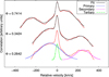 |
Fig. 1 A sample of cross-correlation functions of different orbital phases and their fits with the sum of three Gaussian functions. We also indicate the peaks raised by different components with different lines and colors. |
2.4 Light-curve modeling
The light curves were simultaneously analyzed with the radial velocities using the Wilson-Devinney-code-based program PHOEBE2 (Prsa & Zwitter 2005), in order to create a physical model of VW Cephei and to determine its physical parameters. The surface-averaged effective temperature of the primary component (Teff,1) and the relative temperatures of the starspots were kept fixed at 5050 K as in Kaszás et al. (1998), and 3500 K as in Hendry & Mochnacki (2000), respectively. We assumed that the orbit is circular and the rotation of the components is synchronous, therefore, the eccentricity was fixed at 0.0, and the synchronicity parameters were kept at 1.0. For the gravity darkening coefficients and bolometric albedos, we adopted the usual values for contact systems: g1 = g2 = 0.32 (Lucy 1967) and A1 = A2 = 0.5 (Rucinski 1969), respectively. The following parameters were varied during the modeling: the effective temperature of the secondary component (Teff,2), the inclination (i), the mass ratio (q), the semi-major axis (a), the gamma velocity (vγ), the luminosities of the three components, and the coordinates and radii of starspots. The limb darkening coefficients were interpolatedfor every iteration from PHOEBE’s built-in tables using the logarithmic limb darkening law.
Light curves obtained on the given nights are plotted in Figs. 3, A.1–A.4 along with their model curves fitted by PHOEBE and the corresponding geometrical configurations in different orbital phases. The residuals are mostly in the range of ±0.02 magnitudes, which is comparable to our photometric accuracy. One can see that the difference of the two maxima changes slightly from night to night in each filter. This variation suggests ongoing surface activity, and it is treated by assuming cooler spots on the surface of the components. The final model and spot parameters are listed in Tables 1 and 2, respectively.
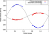 |
Fig. 2 Radial velocity curve of VW Cephei with the fitted PHOEBE model. We note that the formal errors of the single velocity points (see Table C.1) are smaller than their symbols. |
2.5 Spectrum synthesis
In order to analyze the chromospheric activity of the system, we constructed synthetic spectra for every observed spectra. Forspectrum synthesis, we used Robert Kurucz’s ATLAS9 (Kurucz 1993) model atmospheres selecting different temperatures (4500–6500 K, with 250 K steps). The model spectra were Doppler-shifted and convolved with the broadening functions associated with the observed orbital phases that were computed with the WUMA4 program. As in Kaszás et al. (1998), the tertiary component is also well-resolved in our cross-correlation functions (Fig. 1), which means that its contribution is not negligible. Accounting for this third component, a T = 5000 K, log g = 4.0 model was used: it was Doppler-shifted, then convolved with a simple Gaussian function applying the FWHM of the transmission function of the spectrograph. A scaled version of this model spectrum (assuming that the third component gives 10% of the total luminosity, based on Kaszás et al. 1998) was added to the contact binary model spectrum to mimic the presence of the tertiary component. We fitted the produced synthetic spectra with different temperatures to the observed data (leaving out the Hα-region), and found that T = 5750 K and log g = 4.0 gives the best-fit model. This temperature value corresponds to the flux-averaged mean surface temperature, and it is very similar to that found by Hendry & Mochnacki (2000) for the unspotted mean surface temperature of VW Cep. The best-fit model spectra were then subtracted from the observed ones at every epoch. Finally, we measured the EWs of the Hα-profile on the residual (observed minus model) spectra using the IRAF/splot task. It is hard to fit the Hα-line of the components with the usual Gaussian- or Voigt-profiles on the residual spectra, so we chose the direct integration of the equivalent widths. We assumed that the uncertainties of the EW measurements mostly come from the error of the continuum normalization, hence they were determined by the RMS of the relative differences between the observed and synthetic spectra outside the Hα-region.
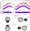 |
Fig. 3 SDSS g′r′i′ light curves of VW Cephei on 8 August 2014 along with the fitted PHOEBE models and the corresponding geometrical configuration and spot distribution in different orbital phases. |
Physical parameters of VW Cep according to our PHOEBE light- and radial velocity curve models compared to the previous results of Kaszás et al. (1998).
Spot parameters from the light curve models of single nights.
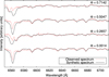 |
Fig. 4 A sample of observed (dashed line) and synthesized (solid line) spectra of VW Cephei in different orbital phases. |
3 The activity of VW Cep
A sample of our observed and synthetic spectra is plotted in Fig. 4, while a more detailed view of the Hα-region along with the difference spectra is available in Appendix D (Figs. D.1 and D.2). We can see an obvious excess in the Hα line profile, which strongly suggests ongoing chromospheric activity. The excess belongs mainly to the line component of the more massive primary star, while there is no sign of clear emission in the line component of the secondary star. This implies that the chromosphere of the primary star is much more active, consistent with our light curve models where we assumed that spots are located on the primary.
In Fig. 5, we plotted the determined EW values as a function of the orbital phase. As can be seen, the values on the two consecutive nights in 2016 are almost the same; the small differences may be caused by continuum normalization effects (as noted by Kaszás et al. 1998, 3% error in the continuum can result in a 0.3 Å error in the EWs).
The light curves obtained in 2014 (Figs. 3, A.1 and A.2) and 2016 (Figs. A.3 and A.4) clearly show a smaller maximum brightness at phase Φ = 0.25. Without spectroscopy, one would most probably think that it is caused by a spot (or a group of spots) on the surface of the primary component when it is moving towards us, or on the secondary component when it is moving away from us. Nevertheless, if we analyze the EWs versus orbital phase diagram (Fig. 5), we can see two peaks centered at the phases of Φ = 0.1 and Φ = 0.5. This impliesthat enhanced chromospheric activity is occurring at these two phases, so we should expect spots there. Hence, we modeled the light curves with two spots (on the regions of the primary that faces the observer at Φ = 0.1 and Φ = 0.5 phase, respectively). A better fit was obtained using a two-spots configuration in all three filter bands than in the case of a single spotted region placed at Φ = 0.25 (PHOEBE’s built-in cost function gives an approximately two times higher value if we use one spot instead of two, keeping the same orbital configuration). We note that the single-spot fit can be improved by increasing the temperature difference of the two stars up to 600 K; however, such a high value of Δ T is unlikely in the case of aW UMa star, and the result of the fitting is still worse than assuming two spots. According to the best-fit PHOEBE models, there is a larger spotat Φ = 0.5 phase when we see a higher peak on the EW-phase diagram (Fig. 5), and a smaller spot at Φ = 0.1 when we seea lower peak. This clearly shows that there is a correlation between spottedness and the strength of the chromospheric activity. In order to visualize this correlation, we subtracted spotless synthetic light curves from the observed light curves obtained in 2016 and plotted the residuals in Fig. 6. One can see that the shape of Fig. 6 is very similar to Fig. 5.
As one can see in Figs. 3, A.1, A.2, A.3, and A.4, the model spots we used are located at relatively high latitudes on the primary component. Although, in general, latitudinal information of spots cannot be reliably extracted from light-curve modeling (Lanza & Rodonó 1999), earlier studies concluded that high-latitude spots are expected on rapidly rotating stars (Schüssler & Solanki 1992; Schüssler et al. 1996; Holzwarth & Schüssler 2003).
In our PHOEBE models, spots are situated mainly at two longitudes separated by nearly 180 degrees in line with the center of the components, which is consistent with the model of Holzwarth & Schüssler (2003). They showed that this is expected in active close binaries, because the tidal forces can alter the surface distribution of erupting flux tubes and create spot clusters on the opposite sides of the active component. Such active longitudes were found in other close binaries by Oláh (2006).
This kind of longitudinal distribution of spots could also be the sign of the so-called flip-flop phenomenon, which is explained as the combination of a nonaxisymmetric dynamo mode with an oscillating axisymmetric mode in case of a star with spherical shape (Elstner & Korhonen 2005). This phenomenon has been observed on numerous stars (mainly on FK Com and RS CVn systems, but also on the Sun and on young solar-like stars) that show two active longitudes on their opposite hemispheres with alternating spot activity level (e.g., Jetsu et al. 1993; Vida et al. 2010). In these cases, the observed variations of the surface activity are somewhat periodic; flip cycles are usually in the range of a few years to a decade. Activity cycles of contact binaries have also been assumed previously, based on the cyclic variations of minima seen on O–C diagrams, and on the seasonal variations of the light curves, especially of the differences of light-curve maxima within a cycle (Kaszás et al. 1998; Borkovits et al. 2005). Recently, Jetsu et al. (2017) presented a general model for the light curves of chromospherically active binary stars. According to them, probably all such systems have these two active longitudes with cyclic alternation in their activity (we note however, that they analyzed only RS CVn systems). Our data cover a relatively short time and we can’t see any large changes in the spot strengths. The only convincing evidence we found is shown in Fig. 1 of Kaszás et al. (1998), where the authors plotted the seasonal light curves of VW Cephei. One can see the relative changes in the photometric maxima on a scale of 3–4 years which could be explained by changes in the spot strengths. The only contact binary system with a detected flip-flop phenomenon is HH UMa (based on the seasonal variations of light curves, see Wang et al. 2015). Nevertheless, the observed light-curve variations of HH UMa are very similar to those that can be seen in the case of VW Cep (see in Fig. 1 of Kaszás et al. 1998). Thus, it could be argued that the presence of the flip-flop phenomenon is a viable hypothesis even in the cases of close binary stars.
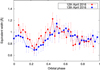 |
Fig. 5 EWs of the Hα emission line profile measured on different nights in the function of orbital phase. For determining the EW values, we subtracted synthetic spectra from the observed ones at every epoch (see the text for details). |
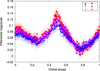 |
Fig. 6 Residuals of light curves measured in 2016 compared to spotless synthetic light curves. |
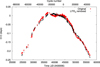 |
Fig. 7 O–C diagram before (red diamonds) and after the subtraction of the visually observed LITE of the 3rd body. Cycle numbers areshown on the top horizontal axis. |
Times of primary and secondary minima obtained from our photometric data.
4 O–C analysis
In order to analyze the periodic variations of VW Cep, we constructed the O–C diagram of the system. For this purpose, we downloaded all the minima times from the O–C gateway webpage3 created by Anton Paschke and BC. Lubos Brát. Furthermore, we collected all other available data points from IBVS, BBSAG, BAA-VSS and BAV issues, and, finally, we added the latest points from our measurements (see Table 3).
We only selected the most reliable measurements obtained with photoelectric and CCD devices. For the calculations, we used the reference epoch and period from the GCVS catalog (Kreiner & Winiarski 1981):

The final diagram, which includes the times of both primary and secondary minima, contains 1620 data points (Fig. 7).
The O–C diagram has a clearly visible negative parabolic trend shape. Kaszás et al. (1998) fitted the long-term period decrease with a parabolic function getting Δ P∕P = −0.58 × 10⁻⁹. They assumed that this phenomenon is caused by a conservative mass transfer from the primary (more massive) component to the secondary one and determined a mass transfer rate of Δ M = 1.4 × 10⁻⁷ M⊙ yr−1. They conclude that the large rate of period decrease and of the mass transfer indicate that this phenomenon should be temporary. After the subtraction of the parabola, the residual contains a periodic variation which was explained with the presence of a light-time effect (LITE) by several authors (Hill 1989; Kaszás et al. 1998; Pribulla et al. 2000; Zasche & Wolf 2007). This LITE is probably caused by the third body orbiting around the center of mass of the VW Cep AB. Hershey (1975) confirmed the existence of this tertiary component, but the observed amplitude of the LITE is larger than expected from its orbital elements. After subtracting the effect of the third body, the residual shows additional periodic variations. Kaszás et al. (1998) proposed two possible explanations for this cyclic behavior: (i) perturbation of orbital elements induced by the tidal force of the third body, and (ii) geometric distortions caused by magnetic cycles (Applegate mechanism; Applegate 1992).
Regarding the significantly larger number of data points (collected in the last 20 years), we decided to re-analyze the rate of period decrease. Furthermore, we propose new explanations for the different cyclic variations. For these purposes, we removed the LITE of thevisually observed tertiary component as was also done in Kaszás et al. (1998); see Fig. 7.
As a first approach, the O–C diagram was fitted by a quadratic polynomial (Fig. 8). The residual shows periodic variations, and, moreover, large deviations in the early years of observations (we note that it is difficult to estimate theuncertainties of these values), as well as near and after 20 000 cycles. Then we fitted the data with a cubic polynomial, which resulted in a smaller sum of squared residuals. The deviations decrease in the intervals mentioned before, which may suggest that the rate of period decrease is changing in time. If we assume that the period decrease is due to mass transfer, then the period changes and the mass-transfer rates can be calculated (see Table 4), which are of the same order as calculated by Kaszás et al. (1998). The cubic fit yielded positive numbers both in the variation of period change and of mass-transfer rate, which implies that the efficiency of the mass transfer from the more-massive component is decreasing, in agreement with the previous expectations.
The fact that the higher-order polynomial has a better fit to the O–C diagram could be the consequence of a periodic variation, which is not covered yet due to its very long time-scale. To incorporate this assumption, we subtracted the LITE ofthe known third body, then we assumed that the long-term variation is caused by a hypothetical fourth bodyand fitted the residual diagram with a LITE. The best-fit curve generated by using the nonlinear least-squares method can be seen in Fig. 9. The fitted parameters are listed in Table 5.
Defining m4 as the mass of the fourth body, the mass function is
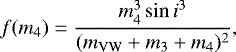 (1)
(1)
where mVW and m3 are the mass of VW Cep AB and the known third body, respectively, and i is the inclination. The amplitude of the O–C is:
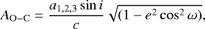 (2)
(2)
where a1,2,3 is the semi-major axis of the common center of mass of VW Cep AB and the third body around the hypothetical fourth body, c is the speed of light, e is the eccentricity, and ω is the argument of periapsis. Combining Eq. (1) and Kepler’s third law, the mass function of the fourth body can be also calculated as:
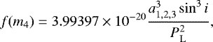 (3)
(3)
where the semi-major axis is in km, the period is in days, and the mass function yields the result in M⊙. Calculated semi-major axes and masses of the fourth body (assuming different values of inclination) can be found in Table 6. We used 1.47 M⊙ (this paper) and 0.74 M⊙ (Zasche 2008) for the total mass of VW Cep AB and for the mass of the third component, respectively.
According to celestial mechanics (e.g., Reipurth & Mikkola 2012), such a four-body system can only be stable if the outer periastron distance is at least 5–10 times larger than the inner apastron distance. The semi-major axis of the orbit of VW Cep AB around the common center of mass is (647.76 ± 29.92) × 106 km (Zasche & Wolf 2007). The semi-major axis of the third body, calculated from the mass ratio m3 /mVW, is (1199.23 ± 55.39) × 106 km. The sum of the two values is (1846.99 ± 60) × 106 km. If we assume that the distance of the fourth body must be at least 7.5 times (average of the criterion given by Reipurth & Mikkola 2012) larger than the inner system’s periastron distance, then we get a1,2,3 ≥ (13 852.4 ± 500) × 106 km. Considering the calculations in Table 6, we can put constraints on inclination, i ≲ 30°, which is in agreement with the assumed inclination of the third body (33.6 ± 1.2°; Zasche & Wolf 2007). Using this value, the mass of the fourth body will be at least 23.9 M⊙. A star with such a large mass should be detectable within the distance of VW Cep, so we note that this object, if it exists, should be a black hole. Such a massive object was recently proposed as an explanation of the periodic variation seen on the O–C diagram of an RR Lyrae binary candidate in Sódor et al. (2017).
The orbital speed of the common center of mass of VW Cep AB and the third body around the center of mass of the four-body system is:
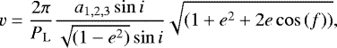 (4)
(4)
where f is the true anomaly. The projection to the plane of the sky is:
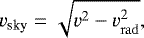 (5)
(5)
where
![Mathematical equation: \begin{equation*} v_{\mathrm{rad}} = \frac{2\pi}{P_{\mathrm{L}}} \frac{a_{1,2,3}\sin{i}}{\sqrt{1-e^2}}\bigg[\cos{(f+\omega)}+e \cos{(\omega)}\bigg], \end{equation*}](/articles/aa/full_html/2018/04/aa31402-17/aa31402-17-eq7.png) (6)
(6)
which is the radial velocity, from which the proper motion is:
![Mathematical equation: \begin{equation*} \mu [{}^{\prime\prime}\, \mathrm{yr}^{-1}] = \frac{v_{\mathrm{sky}} [{\mathrm{km\, s}^{-1}}]}{4.74 \cdot d[\textrm{pc}]}. \end{equation*}](/articles/aa/full_html/2018/04/aa31402-17/aa31402-17-eq8.png) (7)
(7)
The parallax of the VW Cep AB system is 36.25 ± 0.58 mas (van Leeuwen 2007), which leads to a distance of  pc. Proper motion values calculated with different inclinations are listed in Table 6. In the literature, two measured proper motions can be found (Table 7), which are of the same order as in our calculations assuming a low value of inclination. We checked the proper motion values of the nearby stars in order to investigate if such a large value is common in that field or not. We found only one object (LSPM J2040+7537) with a proper motion in this order of magnitude. Unfortunately, we have not found any measured parallax in the literature, but the large angle distance (729.02′′) and the relatively low brightness (R = 15.2 mag) suggest that this star is at a large physical distance from VW Cep. Thus, the measured large proper motion values may be partially explained by the presence of a fourth body.
According to previous papers, the gamma velocity of VW Cephei is continuously changing in time; however, a satisfying explanation for this has yet to be found. Zasche (2008) tried to explain this variation based on the four available gamma velocities in the literature with two different models: (i) the presence of a third and a fourth component in the system without mass transfer between the primary and secondary, or (ii) the presence of a third component in the system with mass transfer between the primary andsecondary. He concluded that the first approach gives a better fit by 12%, but the fit is still not satisfactory and although the assumed fourth component should be detectable, a candidate has yet to be found. More precise data and more sophisticated modeling methods are necessary to solve this problem. However, our new value of vγ seems to be in disagreement with the predictions of Zasche (2008).
Kaszás et al. (1998) Fourier-analyzed the residual after subtracting both a parabolic term and a LITE component corresponding to the orbital elements of the third body (Hershey 1975). They found two significant peaks, one close to the orbital period of the third body (1.29 × 10⁻⁴ day−1), and another one (3.59 × 10⁻⁴ day−1) that was linked to the magnetic activity cycle. We recalculated the Fourier spectrum using all published up-to-date data points, and the same fitting parameters as Kaszás et al. (1998) in order to check whether the mentioned peaks are still visible or not (Fig. 10; marked with an arrow). Additionally, we calculated the Fourier spectrum after subtracting our quadratic and cubic terms as well as the effect of the third body. As one can see, the shorter period has nearly the same amplitude and frequency in all spectra except the cubic case, where the amplitude is smaller by a factor of 2. The peak in the Fourier spectrum of the data after the subtraction of LITE3 and LITE4 is present with nearly the same parameters as in the case of fitting a cubic function. Regarding the longer period, the amplitude of the corresponding peak is larger, and, moreover, another peak appears with a period of 73.52 yr in the longer dataset (Fig. 10b). Such a period caused by the LITE of another hypothetical fourth body has also been proposed by Zasche (2008), but in the case of our new quadratic fit, the peak has disappeared or been delayed, which means that this could be an artifact.
Applegate (1992) proposed a mechanism to explain the orbital period changes of eclipsing binaries. Due to the gravitational coupling, the variation of the angular momentum distribution can modify the orbital parameters (such as the semi-major axis, or the orbital period). The shape of the active component of the binary can be periodically distorted by its magnetic cycle of a field of several kiloGauss. Such a process cannot be excluded in the case of VW Cep because of the photospheric and chromospheric activity of the components observed in the X-ray range (Gondoin 2004; Huenemoerder et al. 2006; Sanz-Forcada et al. 2007). We calculated the value of the orbital period modulation (ΔP), the angular momentum transfer (ΔJ) and the subsurface magnetic field strength (B) required to establish the observed period changes in the O–C diagram (Table 8) as follows (Applegate 1992):
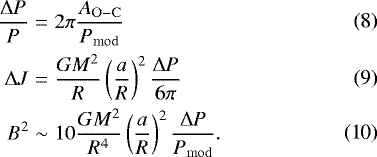
We used the values of a = 1.412 × 10⁶ km (semi-major axis), P = 0.2783 d (orbital period), M1 = 1.13M⊙, M2 = 0.34M⊙ (masses of the primary and the secondary components), R1 = 0.99R⊙, R2 = 0.57R⊙ (radii of the primary and secondary components), respectively. The AO-C values were calculated using Eq. (2) and taken from the Fourier-spectrum, respectively. As can be seen, the calculated subsurface magnetic field strength is lower in the case of the shorter modulation. In Sect. 3, we showed that the primary, more massive component is covered by cool spots, emerged as a result of the magnetic activity. If we assume that the 7.62-year-long modulation in the Fourier spectrum is linked to the magnetic cycle of VW Cep, then the required subsurface magnetic field strength for establishing the variation is higher than 20 kG. If this field strength becomes lower even by two or three orders of magnitude at the surface, it should be detectable with spectropolarimetric observations (see Donati & Landstreet 2009); however, the detection of strength and variation of this magnetic field (via e.g., Zeeman effect) would be a challenging task due to the large rotational broadening of spectral lines (approx. 3.3 Å at 5000 Å).
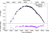 |
Fig. 8 Fittedquadratic (dashed blue curve) and cubic (dotted magenta curve) polynomial to the O–C diagram (top) and their residuals (bottom). Cycle numbers are shown on the top horizontal axis. |
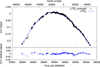 |
Fig. 9 FittedLITE of the hypothetical 4th body to the O–C diagram without the LITE of the known 3rd body (top) and the residual (bottom). Cycle numbers are shown on the top horizontal axis. |
O–C diagram: fitted (top four rows) and calculated (bottom four rows) parameters.
Fitted parameters of the LITE of the hypothetical fourth body.
Calculated orbital parameters, masses and proper motions of the hypothetical 4th body assuming different inclination angles.
Measured proper motion values from the literature.
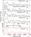 |
Fig. 10 Fourier spectra of the O–C diagrams. From top to bottom: (a) after the subtraction of the parabolic trend (following Kaszás et al. 1998) and the visually observed LITE of the third body using data points before MJD 50 000, (b) same as (a), but using the full dataset, (c) after the subtraction of our quadratic fit along with the LITE of the third body, (d) after the subtraction of our cubic fit along with the LITE of the third body, (e) after the subtraction of the LITE of the third body and (f) after the subtraction of the LITE of the hypothetical fourth body. We highlight the different ranges of the vertical axes. The insert in the fifth panel shows the spectral window. |
5 Summary
We obtained 69 new medium-resolution spectra of VW Cephei along with two new light curves in April 2016, and along with three additional light curves from two years earlier. We analyzed the period variation and the apparent activity of the system. We modeled our new light curves and radial velocity curve simultaneously using the PHOEBE code and also derived ten new times of minima, which were used to construct a new, extended O–C diagram of the system. We redetermined the physical parameters of the system from our models, which are consistent with those in Kaszás et al. (1998). All observed spectra were compared to synthetic spectra. We then measured the EWs of the Hα profile on every difference spectra. According to the light curve and spectral models, it is confirmed that both photospheric and chromospheric activity are mostly occurring on the more massive primary component of the system. Based on our PHOEBE models, the spot distribution seems to be stable, and spots are located on the two opponent hemispheres of the primary in line with the center of both components. The spots also have different sizes or different temperatures which causes the O’Connell effect on the light curves. The EWs of the Hα line show enhanced chromospheric activity in two phases where the spots actually turn in our line of sight, which means that there is a correlation between spottedness and the strength of the chromospheric activity. We propose that this kind of spot distribution might be a consequence of the so-called flip-flop phenomenon, which was recently detected in an other contact binary, HH UMa by Wang et al. (2015). We note that the changes on the light curves of different seasons in Fig. 1 of Kaszás et al. (1998) can also support this hypothesis. Nevertheless, more observationsare still needed for confirmation, especially both photometric and spectroscopic measurements taken simultaneously.
After subtracting the LITE of the previously known third component from the O–C diagram, our period analysis shows that the mass-transfer rate is decreasing, which means that this effect is expected to be temporary as was proposed earlier by Kaszás et al. (1998). In the Fourier spectrum of the O–C diagram, we found a significant peak at about 185 years and also detected a peak at 7.62 years, which was connected to the magnetic activity cycling by Kaszás et al. (1998). We tested two previously suggested hypotheses to explain these peaks: (i) the presence of an additional fourth component in the system, and (ii) ongoing geometrical distortions by magnetic cycle. The supporting fact of the former is that a cubic polynomial fits the O–C diagram better than a quadratic one. This could indicate a longer periodic variation that is not yet fully covered by the observations. We treated the long-term variation as LITE and assumed that this might be a consequence of the presence of a fourth body, whose mass would be at least 23.9 M⊙ (assuming i ≲ 30°). This scenario could also be a partial explanation of the large proper motion values of VW Cep. The other scenario we analyzed is that the period variation could be the consequence of the Applegate-mechanism; from our calculations, the necessary strength of the subsurface magnetic field required to maintain the observed period variation is higher than 20 kG. Nevertheless, the available data suggest that mass transfer from the more massive primary to the less massive secondary star (with a slowly decreasing mass-transfer rate) is the most probable explanation for the observed period variation of VW Cep.
Calculated angular momentum transfer (ΔJ) and the subsurface magnetic field strength (B) required to establish the observed period changes.
Acknowledgements
We would like to thank our anonymous referee for his/her valuable suggestions, which helped us to improve the paper. This project has been supported by the Lendület grant LP2012-31 of the Hungarian Academy of Sciences and the Hungarian National Research, Development and Innovation Office, NKFIH-OTKA K-113117 and K-115709 grants. K. Vida acknowledges the Hungarian National Research, Development and Innovation Office grants OTKA K-109276, and supports through the Lendület-2012 Program (LP2012-31) of the Hungarian Academy of Sciences, and the ESA PECS Contract No. 4000110889/14/NL/NDe. K. Vida is supported by the Bolyai János Research Scholarship of the Hungarian Academy of Sciences.
Appendix A: Light curves and spot configurations
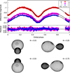 |
Fig. A.1 SDSS g′r′i′ light curves of VW Cephei on 9 August 2014 along with the fitted PHOEBE models and the corresponding geometrical configuration and spot distribution in different orbital phases. |
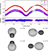 |
Fig. A.2 SDSS g′r′i′ light curves of VW Cephei on 10 August 2014 along with the fitted PHOEBE models and the corresponding geometrical configuration and spot distribution in different orbital phases. |
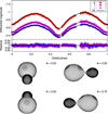 |
Fig. A.3 SDSS g′r′i′ light curves of VW Cephei on 20 April 2016 along with the fitted PHOEBE models and the corresponding geometrical configuration and spot distribution in different orbital phases. |
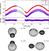 |
Fig. A.4 SDSS g′r′i′ light curves of VW Cephei on 21 April 2016 along with the fitted PHOEBE models and the corresponding geometrical configuration and spot distribution in different orbital phases. |
Appendix B: Checking the limitations of the cross-correlation technique
We used the parameters derived by Kaszás et al. (1998) for these calculations. A broadening function of the Φ = 0.2642 phase is plotted along with the fitted Gaussian functions in Fig. B.1. The radial velocity points measured atthe maxima of the two components of the broadening function are plotted in Fig. B.2 along with the best-fit sine curves (solid line) and the theoretical curve of the system computed from the input parameters (dashed line). There are only minor differences between the two curves, and the measured mass ratio (qmeasured = 0.344) has only a 1.8% relative difference compared tothe original value (qoriginal = 0.35).
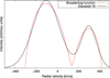 |
Fig. B.1 A broadening function of the Φ = 0.2642 phase and its fit with the sum of two Gaussian functions. |
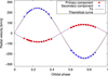 |
Fig. B.2 Radial velocity curve of VW Cephei measured on the theoretical broadening functions. The solid line shows the fitted sine functions and the dashed line shows the theoretical velocity curve. |
Appendix C: Radial velocities
Newly derived radial velocities and their errors.
Appendix D: Hα profiles and difference spectra
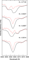 |
Fig. D.1 Hα region of the previous sample of observed and synthesized spectra of VW Cephei in different orbital phases. |
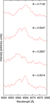 |
Fig. D.2 Difference spectra around the Hα region of the previous sample of observed and synthesized spectra of VW Cephei in different orbital phases. |
References
- Anderson, L., Raff, M., & Shu, F. H. 1980, IAU Symp., 88, 485 [NASA ADS] [Google Scholar]
- Applegate, J. H. 1992, ApJ, 385, 621 [NASA ADS] [CrossRef] [Google Scholar]
- Baliunas, S. L., Donahue, R. A., Soon, W. H. et al. 1995, ApJ, 438, 269 [NASA ADS] [CrossRef] [Google Scholar]
- Binnendijk, L. 1967, Publ. Dom. Astrophys. Obs., 13, 27 [NASA ADS] [Google Scholar]
- Binnendijk, L. 1970, Vist. Astron., 12, 217 [Google Scholar]
- Borkovits, T., Elkhateeb, M. M., Csizmadia, Sz. et al. 2005, A&A, 441, 1087 [NASA ADS] [CrossRef] [EDP Sciences] [Google Scholar]
- Donati, J.-F., & Landstreet, J. D., 2009, ARA&A, 47, 333 [NASA ADS] [CrossRef] [MathSciNet] [Google Scholar]
- Eggleton, P. P., & Kiseleva-Eggleton, L. 2001, ApJ, 562, 1012 [NASA ADS] [CrossRef] [Google Scholar]
- Elstner, D., & Korhonen, H. 2005, AN, 326, 278 [Google Scholar]
- Frasca, A., Sanfilippo, D., & Catalano, S. 1996, A&A, 313, 532 [NASA ADS] [Google Scholar]
- Gondoin, P. 2004, A&A, 415, 1113 [NASA ADS] [CrossRef] [EDP Sciences] [Google Scholar]
- Heckert, P. A., & Ordway, J. I. 1995, AJ, 109, 2169 [NASA ADS] [CrossRef] [Google Scholar]
- Hendry, P. D., & Mochnacki, S. W. 2000, ApJ, 531, 467 [NASA ADS] [CrossRef] [Google Scholar]
- Hershey, J. L. 1975, AJ, 80, 662 [NASA ADS] [CrossRef] [Google Scholar]
- Hill, G. 1989, A&A, 218, 141 [NASA ADS] [Google Scholar]
- Holzwarth, V., & Schüssler, M. 2003, A&A, 405, 303 [NASA ADS] [CrossRef] [EDP Sciences] [Google Scholar]
- Huenemoerder, D. P., Testa, P., & Buzasi, D. L. 2006, ApJ, 650, 1119 [NASA ADS] [CrossRef] [Google Scholar]
- Jetsu, L., Pelt, J, & Tuominen, I. 1993, A&A, 278, 449 [NASA ADS] [Google Scholar]
- Jetsu, L., Henry, G. W., & Lehtinen, J. 2017, ApJ, 838, 122 [NASA ADS] [CrossRef] [Google Scholar]
- Kaszás, G., Vinkó, J., Szatmáry, K., et al. 1998, A&A, 331, 231 [NASA ADS] [Google Scholar]
- Kreiner, J. M., & Winiarski, M. 1981, Acta Astron., 31, 351 [NASA ADS] [Google Scholar]
- Kurucz, R. 1993, ATLAS9 Stellar Atmosphere Programs and 2 km/s Grid, Kurucz CD-ROM No. 13 (Cambridge, MA: Smithsonian Astrophysical Observatory) [Google Scholar]
- Kwee, K. K. 1966, Bull. Astron. Inst. Netherlands, 18, 448 [NASA ADS] [Google Scholar]
- Lanza, A. F., & Rodonó, M. 1999, in Solar and Stellar Activity: Similarities and Differences, eds. C. J. Butler, & J. G. Doyle, ASP Conf. Ser., 158, 121 [NASA ADS] [Google Scholar]
- Lenz, P., & Berger, M. 2005, Commun. Asteroseismol., 146, 53 [NASA ADS] [CrossRef] [Google Scholar]
- Lucy, L. B. 1967, Z. Astrophys., 65, 89 [Google Scholar]
- Lucy, L. B. 1968, ApJ, 151, 1123 [NASA ADS] [CrossRef] [Google Scholar]
- Mullan, D. J. 1975, ApJ, 198, 563 [NASA ADS] [CrossRef] [Google Scholar]
- Oláh, K. 2006, Ap&SS, 304, 145 [NASA ADS] [CrossRef] [Google Scholar]
- Oláh, K., & Strassmeier, K. G. 2002, Astron. Nachr., 323, 361 [NASA ADS] [CrossRef] [Google Scholar]
- Popper, D. M. 1948, ApJ, 108, 490 [NASA ADS] [CrossRef] [Google Scholar]
- Pribulla, T., Chochol, D., Tremko, J., et al. 2000, CoSka, 30, 117 [NASA ADS] [Google Scholar]
- Pribulla, T., & Rucinski, S. M. 2006, AJ, 131, 2986 [NASA ADS] [CrossRef] [Google Scholar]
- Prsa, A., & Zwitter, T. 2005, ApJ, 628, 426 [NASA ADS] [CrossRef] [Google Scholar]
- Pustylnik, I., & Sorgsepp, L. 1976, Acta Astron., 26, 319 [NASA ADS] [Google Scholar]
- Reipurth, B., & Mikkola, S. 2012, Nature, 492, 221 [Google Scholar]
- Roeser, S., & Bastian, U. 1988, A&AS, 74, 449 [NASA ADS] [Google Scholar]
- Rucinski, S. M. 1969, Acta Astron., 19, 245 [Google Scholar]
- Rucinski, S. M. 1973, Acta Astron., 23, 79 [NASA ADS] [Google Scholar]
- Rucinski, S. M. 1974, Acta Astron., 24, 119 [NASA ADS] [Google Scholar]
- Rucinski, S. 2010, in International Conference on Binaries: In celebration of Ron Webbink’s 65th Birthday, eds. V. Kalogera, & M. van der Sluys, AIP Conf. Proc., 1314, 29 [NASA ADS] [CrossRef] [Google Scholar]
- Samus N. N., Kazarovets E. V., Durlevich O. V., Kireeva N. N., & Pastukhova E. N. 2017, Astron. Rep., 61, 80 [NASA ADS] [CrossRef] [Google Scholar]
- Sanad, M. R., & Bobrowsky, M. 2014, New Astron., 29, 47 [NASA ADS] [CrossRef] [Google Scholar]
- Sanz-Forcada, J., Favata, F., & Micela, G. 2007, A&A, 466, 309 [NASA ADS] [CrossRef] [EDP Sciences] [Google Scholar]
- Schilt, J. 1926, ApJ, 64, 221 [Google Scholar]
- Schüssler, M., & Solanki, S. K. 1992, A&A, 264, L13 [NASA ADS] [Google Scholar]
- Schüssler, M., Caligari, P., Ferriz-Mas, A., Solanki, S. K., & Stix, M. 1996, A&A, 314, 503 [NASA ADS] [Google Scholar]
- Soubiran, C., Jasniewicz, G., Chemin, L. et al. 2013, A&A. 552, A64 [CrossRef] [EDP Sciences] [Google Scholar]
- Sódor, Á., Skarka, M., Liska, J., & Bognár, Zs. 2017, MNRAS, 465, L1 [NASA ADS] [CrossRef] [Google Scholar]
- van’t Veer, F. 1973, A&A, 26, 357 [NASA ADS] [Google Scholar]
- van Leeuwen, F., 2007, A&A, 474, 653 [NASA ADS] [CrossRef] [EDP Sciences] [Google Scholar]
- Vida, K., Oláh, K., Kővári, Zs. et al. 2010, Astron. Nachr., 331, 250 [NASA ADS] [CrossRef] [Google Scholar]
- Vida, K., Korhonen, H., Ilyin, I. V., Oláh, K., Andersen, M. I., & Hackman, T. 2015, A&A, 580, A64 [NASA ADS] [CrossRef] [EDP Sciences] [Google Scholar]
- Wang, K., Zhang, X., Deng, L. et al. 2015, ApJ, 805, 22 [NASA ADS] [CrossRef] [Google Scholar]
- Wilson, O. C. 1978, ApJ, 226, 379 [NASA ADS] [CrossRef] [Google Scholar]
- Yamasaki, A. 1982, Ap&SS, 85, 43 [NASA ADS] [CrossRef] [Google Scholar]
- Zasche, P., & Wolf, M. 2007, Astron. Nachr., 328, 928 [NASA ADS] [CrossRef] [Google Scholar]
- Zasche P. 2008, Doctoral Thesis, Charles University in Prague [Google Scholar]
Image Reduction and Analysis Facility: http://iraf.noao.edu
PHysics Of Eclipsing BinariEs: http://phoebe-project.org/1.0/
O–C gateway: http://var2.astro.cz/ocgate/
All Tables
Physical parameters of VW Cep according to our PHOEBE light- and radial velocity curve models compared to the previous results of Kaszás et al. (1998).
O–C diagram: fitted (top four rows) and calculated (bottom four rows) parameters.
Calculated orbital parameters, masses and proper motions of the hypothetical 4th body assuming different inclination angles.
Calculated angular momentum transfer (ΔJ) and the subsurface magnetic field strength (B) required to establish the observed period changes.
All Figures
|
Fig. 1 A sample of cross-correlation functions of different orbital phases and their fits with the sum of three Gaussian functions. We also indicate the peaks raised by different components with different lines and colors. |
| In the text | |
|
Fig. 2 Radial velocity curve of VW Cephei with the fitted PHOEBE model. We note that the formal errors of the single velocity points (see Table C.1) are smaller than their symbols. |
| In the text | |
|
Fig. 3 SDSS g′r′i′ light curves of VW Cephei on 8 August 2014 along with the fitted PHOEBE models and the corresponding geometrical configuration and spot distribution in different orbital phases. |
| In the text | |
|
Fig. 4 A sample of observed (dashed line) and synthesized (solid line) spectra of VW Cephei in different orbital phases. |
| In the text | |
|
Fig. 5 EWs of the Hα emission line profile measured on different nights in the function of orbital phase. For determining the EW values, we subtracted synthetic spectra from the observed ones at every epoch (see the text for details). |
| In the text | |
|
Fig. 6 Residuals of light curves measured in 2016 compared to spotless synthetic light curves. |
| In the text | |
|
Fig. 7 O–C diagram before (red diamonds) and after the subtraction of the visually observed LITE of the 3rd body. Cycle numbers areshown on the top horizontal axis. |
| In the text | |
|
Fig. 8 Fittedquadratic (dashed blue curve) and cubic (dotted magenta curve) polynomial to the O–C diagram (top) and their residuals (bottom). Cycle numbers are shown on the top horizontal axis. |
| In the text | |
|
Fig. 9 FittedLITE of the hypothetical 4th body to the O–C diagram without the LITE of the known 3rd body (top) and the residual (bottom). Cycle numbers are shown on the top horizontal axis. |
| In the text | |
|
Fig. 10 Fourier spectra of the O–C diagrams. From top to bottom: (a) after the subtraction of the parabolic trend (following Kaszás et al. 1998) and the visually observed LITE of the third body using data points before MJD 50 000, (b) same as (a), but using the full dataset, (c) after the subtraction of our quadratic fit along with the LITE of the third body, (d) after the subtraction of our cubic fit along with the LITE of the third body, (e) after the subtraction of the LITE of the third body and (f) after the subtraction of the LITE of the hypothetical fourth body. We highlight the different ranges of the vertical axes. The insert in the fifth panel shows the spectral window. |
| In the text | |
|
Fig. A.1 SDSS g′r′i′ light curves of VW Cephei on 9 August 2014 along with the fitted PHOEBE models and the corresponding geometrical configuration and spot distribution in different orbital phases. |
| In the text | |
|
Fig. A.2 SDSS g′r′i′ light curves of VW Cephei on 10 August 2014 along with the fitted PHOEBE models and the corresponding geometrical configuration and spot distribution in different orbital phases. |
| In the text | |
|
Fig. A.3 SDSS g′r′i′ light curves of VW Cephei on 20 April 2016 along with the fitted PHOEBE models and the corresponding geometrical configuration and spot distribution in different orbital phases. |
| In the text | |
|
Fig. A.4 SDSS g′r′i′ light curves of VW Cephei on 21 April 2016 along with the fitted PHOEBE models and the corresponding geometrical configuration and spot distribution in different orbital phases. |
| In the text | |
|
Fig. B.1 A broadening function of the Φ = 0.2642 phase and its fit with the sum of two Gaussian functions. |
| In the text | |
|
Fig. B.2 Radial velocity curve of VW Cephei measured on the theoretical broadening functions. The solid line shows the fitted sine functions and the dashed line shows the theoretical velocity curve. |
| In the text | |
|
Fig. D.1 Hα region of the previous sample of observed and synthesized spectra of VW Cephei in different orbital phases. |
| In the text | |
|
Fig. D.2 Difference spectra around the Hα region of the previous sample of observed and synthesized spectra of VW Cephei in different orbital phases. |
| In the text | |
Current usage metrics show cumulative count of Article Views (full-text article views including HTML views, PDF and ePub downloads, according to the available data) and Abstracts Views on Vision4Press platform.
Data correspond to usage on the plateform after 2015. The current usage metrics is available 48-96 hours after online publication and is updated daily on week days.
Initial download of the metrics may take a while.