| Issue |
A&A
Volume 612, April 2018
|
|
|---|---|---|
| Article Number | A114 | |
| Number of page(s) | 8 | |
| Section | Extragalactic astronomy | |
| DOI | https://doi.org/10.1051/0004-6361/201731114 | |
| Published online | 08 May 2018 | |
Building CX peanut-shaped disk galaxy profiles
The relative importance of the 3D families of periodic orbits bifurcating at the vertical 2:1 resonance
Research Center for Astronomy, Academy of Athens,
Soranou Efessiou 4,
115 27
Athens, Greece
e-mail: This email address is being protected from spambots. You need JavaScript enabled to view it.
, This email address is being protected from spambots. You need JavaScript enabled to view it.
Received:
5
May
2017
Accepted:
5
December
2017
Abstract
Context. We present and discuss the orbital content of a rather unusual rotating barred galaxy model, in which the three-dimensional (3D) family, bifurcating from x1 at the 2:1 vertical resonance with the known “frown-smile” side-on morphology, is unstable.
Aims. Our goal is to study the differences that occur in the phase space structure at the vertical 2:1 resonance region in this case, with respect to the known, well studied, standard case, in which the families with the frown-smile profiles are stable and support an X-shaped morphology.
Methods. The potential used in the study originates in a frozen snapshot of an N-body simulation in which a fast bar has evolved. We follow the evolution of the vertical stability of the central family of periodic orbits as a function of the energy (Jacobi constant) and we investigate the phase space content by means of spaces of section.
Results. The two bifurcating families at the vertical 2:1 resonance region of the new model change their stability with respect to that of most studied analytic potentials. The structure in the side-on view that is directly supported by the trapping of quasi-periodic orbits around 3D stable periodic orbits has now an infinity symbol (i.e. ∞-type) profile. However, the available sticky orbits can reinforce other types of side-on morphologies as well.
Conclusions. In the new model, the dynamical mechanism of trapping quasi-periodic orbits around the 3D stable periodic orbits that build the peanut, supports the ∞-type profile. The same mechanism in the standard case supports the X shape with the frown-smile orbits. Nevertheless, in both cases (i.e. in the new and in the standard model) a combination of 3D quasi-periodic orbits around the stable x1 family with sticky orbits can support a profile reminiscent of the shape of the orbits of the 3D unstable family existing in each model.
Key words: chaos / galaxies: bulges / galaxies: kinematics and dynamics / galaxies: structure
© ESO 2018
1 Introduction
Peanut-shaped bulges in N-body simulations have been correlated with the presence of inner Lindblad resonances (ILR; Combes et al. 1990) and are considered to be part of the bars viewed edge-on (Athanassoula & Misiriotis 2002). Many orbital models that have been developed in order to associate the presence of the boxy bulges in galaxies with the presence of orbital families have shown that the observed structures can be built by means of the families introduced in the vertical 2:1 resonance (hereafter vILR) of rotating barred potentials (see e.g. Pfenniger 1984; Pfenniger & Friedli 1991; Patsis et al. 2002).
Briefly, peanut-building families are introduced in the system at the two nearby vILRs, where the planar, central family, x1, experiences a double stability transition. Namely, as the Jacobi constant increases, the initially stable x1 family becomes simple unstable (Contopoulos & Magnenat 1985) and then returns back to stable, that is, we have a S → U → S scheme (see Skokos et al. 2002). At the S → U transition we have a three-dimensional (3D) stable family bifurcating from x1, while at the U → S transition that follows, a 3D unstable family is introduced in the system. In conclusion, the presence of a pair of vILRs gives rise to two 3D families of periodic orbits in the system; one stable, and the other unstable.
In the analytic model of the Ferrers bar (Pfenniger 1984; Patsis et al. 2002), in the double Miyamoto triaxial potential studied by Katsanikas et al. (2013) and in the model of Pfenniger & Friedli (1991) the family of periodic orbits, which is introduced at the S → U transition as stable can be vaguely described as having orbits resembling “frowns” and “smiles” when viewed side-on (we consider both branches of the bifurcating family, which are symmetric with respect to the equatorial plane). In Pfenniger & Friedli (1991) this family changes its stability at larger energies. An exception to the models in which the frown-smile orbits are mainly stable is the model by Mulder & Hooimeyer (1984). However, even in this case the family is introduced as stable and becomes unstable at a nearby energy, beyond but close to the bifurcating point. This family is called BAN by Pfenniger & Friedli (1991) and x1v1 by Skokos et al. (2002) (its symmetric one being called x1v1′). The combination of the two symmetric with respect to the equatorial z = 0 plane side-on projections of x1v1 and x1v1′ will give a ≬ shape. On the other hand, the orbits of the 3D family that is introduced in all these models as unstable (x1v2 in Skokos et al. (2002) and ABAN in Pfenniger & Friedli 1991) appear in the corresponding projection as ∞-shaped. (Here we follow the Skokos et al. 2002, notation.)
Bureau et al. (2006) classify the boxy, peanut-shaped, X-type bulges of edge-on disk galaxies in two morphological classes. They are either CX (centred) or OX (off-centred), depending on whether or not the wings of the X feature cross the centre of the galaxy (CX) or not (OX). A sketch describing the two cases of X is given in Fig. 1. The disk is represented by a horizontal line, since we deal with edge-on views. In (a) the wings of X cross the centre of the disk and thus the sketch describes a CX profile, while in (b) they do not and the profile is an OX one.
Considering that the standard mechanism that builds the observed profiles is the trapping of quasi-periodic orbits in the neighbourhood of stable periodic ones, it is clear that in the studied cases the building of the OX profiles is favoured in the orbital models, since individual, or a number of, stable x1v1 and x1v1′ periodic orbits support this morphology (Patsis et al. 2002). However, recently Patsis & Katsanikas (2014a) emphasised the role of sticky chaotic orbits in building the peanuts and proposed a possible origin for the CX-type profiles. According to that study, such profilescan be built as a combination of 3D quasi-periodic orbits on tori around the planar x1 family together with sticky chaotic orbits emerging from the x1v2 neighbourhood. The latter orbits are led by the unstable manifolds of the unstable x1v2 periodic orbits in the region of the x1v1 tori that flank the x1 island of stability in appropriate (z, pz ) projections of the surfaces of section, if z is the axis of rotation of the system (see Fig. 14 in Patsis & Katsanikas 2014a). These sticky chaotic orbits have during long time intervals hybrid morphologies between x1v1 and x1v2, in which, in most studied cases, the morphology of the unstable periodic orbit prevails; in this case x1v2. Similar portraits of the phase space are encountered in most orbital models that have been studied.
In the majority of the papers where the dynamics at the vILR region is discussed, the 3D bar is represented by a triaxial Ferrers potential (Ferrers 1870) and the stability of the x1v1 and x1v2 families is as described above. On the other hand, in Contopoulos & Harsoula (2013), the order, and thus the stability, of the x1v1 and x1v2 families is reversed. Contopoulos & Harsoula (2013) studied the chaotic diffusion in an N-body model that develops a fast rotating bar. They examined the orbital dynamics in a frozen snapshot of this model in order to show how chaotic orbits, slowly diffusing from the bar region to the region beyond corotation, can support the spiral structure. A peculiarity of the frozen snapshot’s potential was that the stable family was x1v2 and the unstable one was x1v1. Thus we say that their stability has been reversed, compared with the stability of the corresponding families in the analytic potentials.
In the present paper we examine the consequences that the prevalence of stable x1v2 (∞-shaped) periodic orbits in galactic bars could have for their edge-on morphologies. For this purpose we compare the structure of phase space at the vILR of the frozen N-body snapshot in Contopoulos & Harsoula (2013) with that of a standard Ferrers bar (Pfenniger 1984; Patsis et al. 2002, etc.). As a typical case,we consider, the one described in Patsis & Katsanikas (2014a). The goal of this study is to trace the differences in the phase space in the two cases and to find the building blocks each case offers for building peanut-shaped bulges. In Sect. 2 we briefly describe the model, in Sect. 3 we present the structure of the phase space of the model at the vILR, in Sect. 4 we compare it with previous models, in Sect. 5 we compare the variation of the vertical frequencies in the model by Contopoulos & Harsoula (2013) with that of a standard Ferrers bar model, and in Sect. 6 we discuss and summarise our conclusions.
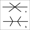 |
Fig. 1 A sketch of the two types of X features appearing in edge-on views of disk galaxies: (a) The CX type, in which the wings of theX cross the centre of the system, and (b) the OX profile, in which the wings of X avoid the centre. |
2 A brief description of the model
We first briefly describe the model with the unusual stability of the 3D bifurcating families at the vILR. The N-body model from which the potential in Contopoulos & Harsoula (2013) originates is described in detail in Harsoula & Kalapotharakos (2009). The code is a smooth potential field scheme along the line of the Allen et al. (1990) numerical algorithm. The model develops in about 0.8 Gyr a bar that lasts almost for 1 Hubble time. The snapshot we consider is taken after 55 half-mass crossing times of the system, which corresponds to about 2.5 Gyr. The V (x, y, z) 3D ‘frozen’ potential is given by the code as an expansion of a bi-orthogonal basis set (Contopoulos & Harsoula 2013). In our analysis we work in the co-rotating with the bar frame of reference. By using a ‘frozen’ potential, our model is an autonomous Hamiltonian system, the Hamiltonian of which can be expressed as
 (1)
where (x, y, z) are the coordinates in a Cartesian frame of reference rotating clockwise around the z-axis with angular velocity Ω p. We have adopted the clockwise rotation in order to be in agreement with the N-body model of Harsoula & Kalapotharakos (2009). In that simulation, the developed barred-spiral structure rotates in such a way that the spiral arms are trailing. In the potential V (x, y, z) of the chosen snapshot the bar is approximately aligned with the y-axis. EJ is the numerical value of the Jacobi constant, hereafter called the energy and dots denote time derivatives. The time unit is taken equal to one half-mass crossing time, while the length unit is taken equal to the half-mass radius (Tsoutsis et al. 2008). The adopted value of the pattern speed used in this study corresponds to Ω p ≈25 km s−1 kpc−1. In all orbital calculations we have used a Runge-Kutta seventh order scheme.
(1)
where (x, y, z) are the coordinates in a Cartesian frame of reference rotating clockwise around the z-axis with angular velocity Ω p. We have adopted the clockwise rotation in order to be in agreement with the N-body model of Harsoula & Kalapotharakos (2009). In that simulation, the developed barred-spiral structure rotates in such a way that the spiral arms are trailing. In the potential V (x, y, z) of the chosen snapshot the bar is approximately aligned with the y-axis. EJ is the numerical value of the Jacobi constant, hereafter called the energy and dots denote time derivatives. The time unit is taken equal to one half-mass crossing time, while the length unit is taken equal to the half-mass radius (Tsoutsis et al. 2008). The adopted value of the pattern speed used in this study corresponds to Ω p ≈25 km s−1 kpc−1. In all orbital calculations we have used a Runge-Kutta seventh order scheme.
The side-on profile of the snapshot of the N-body model is given in Fig. 2a. Heavy dots indicate the location of the unstable Lagrangian points L1 and L2 along the major axis of the bar (y-axis). Frequency analysis in the frozen potential (Contopoulos & Harsoula 2013) has shown that this profile is composed mainly of orbits with frequencies 2:1 and 3:1 on the plane of rotation. Isolating the particles that follow orbits belonging only to the 2:1 class, that is, particles on orbits with frequency 2:1 on the equatorial plane, we construct the profile given in Fig. 2b. The overplotted isodensities clearly indicate that these orbits build a CX-type profile. Since we have an analytic potential for this snapshot we can investigate the dynamical mechanisms that support this structure.
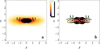 |
Fig. 2 (a) The side-on profile of the N-body model. (b) The side-on profile consisting of orbits belonging to the 2:1 class in the corresponding frozen potential (Contopoulos & Harsoula 2013). The plotted isodensities in (b) emphasise the CX character of the profile. L1 and L2 indicate the location of the unstable Lagrangian points. Darker colour corresponds to more dense regions. |
3 The vILR phase space structure
The interconnections of the families of periodic orbits in the vILR region can be followed by means of the stability diagram that gives the evolution of the stability of the families of periodic orbits as the energy varies (Contopoulos & Magnenat 1985). This is given in Fig. 3. Two stability indices, b1 and b2, characterise the stability of a family with respect to radial and vertical perturbations, respectively, at a given EJ (Broucke 1969).
Figure 3 describes essentially the unusual property of our model that the x1v2 family is introduced in the system in a smaller EJ than x1v1 as stable. It is bifurcated at EJ ≈ − 1.205×10⁶ from x1 at the S → U transition. The family x1v1 is introduced in the system at the slightly larger energy EJ ≈−1.17×10⁶ at the U → S transition. The Lagrangian L1 and L2 points are located at EJ ≈−1.×106, unusually close to the vertical 2:1 resonance region. This is also a notable feature of the model. Both families reach corotation without changing their stability.
In order to describe the structure of the phase space in the presence of the three main families that determine the overall morphology of the thick bar, we chose the energy EJ = − 1.15×10⁶, just beyond the one at which the second family, x1v1, has been introduced in the system. We consider the surface of section y = 0, that is, our consequents are the intersectionsof the orbits with the y = 0 plane with ẏ ≤ 0 (chosen to be like this due to the clockwise rotation) in the six-dimensional phase space. Because of the energy conservation our space of section is reduced to the four-dimensional space (x, z, ẋ, ż). We remind that in symmetric, analytic potentials, the initial conditions of the x1v2 orbits are characterised by z0 = 0, ż ≠ 0, while those of x1v1 by z0≠0, ż =0. Both families have of course also a non-zero initial position on the equatorial plane, that is, x≠ 0 in this case. We note however, that since the potential we study here originates in an N-body model snapshot, the x1 periodic orbits do not start on the x-axis with ẋ = 0, and the bifurcating families are not perfectly symmetric with respect to the equatorial plane. Thus the coordinates that would be zero in the initial conditions of the corresponding families in a symmetric potential are small in the present model, but in general non-zero. For our discussion it is convenient to use (z, ż) projections to describe the results. We chose this particular projection and the specific orbits in order to facilitate the description of our results. Inclusion of more orbits existing in this energy and visualisation of the 4D space of section with other methods as in Patsis & Zachilas (1994) and Katsanikas et al. (2013) would not clarify the structure of phase-space in the present case.
The (z, ż) projection of the 4D space of section for EJ = − 1.15×10⁶ is given in Fig. 4. At this energy we have the stable x1 and x1v2 periodic orbits and the unstable x1v1 one. The location of x1 is (z, ż) ≈ (0, 0). The elliptical “thick” curves around it are the projections of tori that surround it (Katsanikas & Patsis 2011). More precisely they are the tori of the quasi-periodic orbits, which we find by perturbing successively, by increasing Δz, the x1 initial conditions. Because of the asymmetry of the potential, the projections of the tori in the (z, ż) plane will have in general a certain thickness. The orbits on these tori in the configuration space have side-on projections like the one in Fig. 5a. This particular orbit corresponds to the torus coloured blue in Fig. 4, indicated with an arrow labelled with “a”. All orbits similar to the one in Fig. 5a are characterised at (y, z) ≈ (0, 0) by a local maximum in |z|, while there are two local minima on its sides (indicated with arrows in Fig. 5a). With increasing |z| along the ż = 0 axis in Fig. 4 these two local minima in the successive quasi-periodic orbits tend to reach z = 0. This happens when we consider the orbit with the x1 initial conditions, but with |z| ≈ 0.14 instead of 0. In other words the two local minima of the quasi-periodic orbits tend to z = 0 as we approach the initial conditions of the unstable periodic orbits x1v1 and x1v1′ moving along the ż = 0 axis in Fig. 4.
Above and below the region occupied by the x1 tori in Fig. 4 we observe two more regions with tori projected in the (z, ż) plane. They belong to the quasi-periodic orbits around the two members of the stable x1v2 periodic orbit that have ż ≈±573.64 in our velocity units, respectively, and are located close to the z = 0 axis. The side-on projections of the quasi-periodic orbits on the x1v2 tori remind us of the ∞-type morphologyof the x1v2 periodic orbits. Such orbits are characterised at (y, z)≈ (0, 0) by a local minimum in |z| this time. Atypical example is given in Fig. 5b, which corresponds to the red orbit indicated with “b” in Fig. 4.
The ∞-type profile is not the only morphology that can be supported in the side-on view of the model. The sticky chaotic orbits with initial conditions in the neighbourhood of the unstable x1v1 and x1v1′ periodic orbits also provide building blocks for long-lasting structures. In Fig. 4 the consequents that belong to such orbits are roughly projected around the x1 and x1v2 invariant tori building a chaotic layer. The green coloured consequents in this region belong to a typical sticky orbit depicted in Fig. 5c. Its initial condition in the (z, ż) plane is indicated with an arrow close to x1v1′ (Fig. 4, left side, labelled with “c”). Evidently this is an orbit with a hybrid morphology between x1v1 and x1v2. Nevertheless, the x1v1 character prevails.
Besides the individual orbits, we also investigate the morphologies that are supported by the overlapping of several non-periodic orbits associated with one family in different energies. A profile composed by the overplotting of 12 quasi-periodic orbits around stable x1v2 periodic orbits is given in Fig. 6. We consider three orbits at each of the energies EJ = − 1.16, −1.15, −1.14 and − 1.13×10⁶. One of thesetori belongs to an inner torus (like the innermost one in Fig. 4), another one to a torus just before entering into the sticky-chaotic zone that surrounds the tori (like the one labelled with “b” in Fig. 4) and in all cases we consider also a third orbit on a torus between these two. The orbits have been integrated for the time needed to give 30 consequents in the y = 0 space of section. In order to make the effect of the orbital overlapping more discernible, we have converted the twelve overlapping orbits diagram to an image. The orbits are plotted using a constant time step. By constructing the image, we consider the intensity of each pixel to be proportional to the local number density of the points of the orbits in its region. The plotted curves are isodensities that delineate the supported structure. As we can observe in Fig. 6 the overlapping of several quasi-periodic orbits around members of the x1v2 family supports a CX profile. In this case the role of the orbits on tori close to the periodic orbit is important, since they support sharper CX-type X features.
We can build a similar profile by means of the sticky orbits we find by starting with initial conditions in the neighbourhood of the unstable periodic orbits x1v1 and x1v1′. The topology of the phase-space of the model for energies EJ ≥−1.16× 10⁶, in the (z, ż) projection, is similar to the one given in Fig. 4. Thus, a x1v1-like profile can be built by such orbits with energies in the range − 1.17×10⁶ < EJ < −1.12×10⁶. In this case we can combine four sticky orbits that remain close to the projected tori in the (z, ż) plane, like the orbit with the green consequents in Fig. 4. The result is given in Fig. 7a. For constructing this image, we followed the same procedure as in the case of the image in Fig. 6. The orbits are taken at EJ = −1.16, −1.15, −1.14 and − 1.13×10⁶. In this case the profile is of OX type, since the wings of X emerge out of the equatorial plane at |y| > 0.5. We note that the wings remain sharp features, despite the fact that we have used sticky chaotic orbits. The result does not change considerably if we include also 3D quasi-periodic orbits around x1, that is orbits like the one in Fig. 5a, as we can observe in Fig. 7b. Such orbits are by themselves of OX type and their inclusion simply continues the same topology to smaller radii and lower heights.
In summary, the available orbital content for building structures can be either x1v2-like, mainly due to the quasi-periodic orbits around the x1v2 periodic orbit, or x1v1-like, because of the existence of sticky chaotic orbits in the region between and around the invariant tori we encounter in the phase space, at EJ for which both x1v2 and x1v1 exist. The model offers mainly a straightforward mechanism for building CX-type side-on profiles by means of regular orbits such as the one in Fig. 5b. However, by populating the bar of the model with 3D quasi-periodic orbits around x1 (Fig. 5a) and sticky orbits similar to the one in Fig. 5c we can support a frown-smile, OX profile as well.
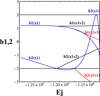 |
Fig. 3 Evolution of the stability indices of the main families at the vILR region. From the mother family x1, bifurcate first the x1v2 as stable and second the x1v1 as unstable. |
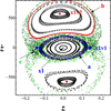 |
Fig. 4 (z, ż) projection of the space of section for the main orbits that participate in building the side-on profile of the model, for EJ = − 1.15×10⁶. Heavy dots indicate the location of x1v1 and x1v2, while the x1 periodic orbit is projected at (z, ż ) ≈ (0, 0). Arrows point to the initial conditions of the orbits given in Fig. 5. |
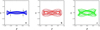 |
Fig. 5 (a) The 3D quasi-periodic orbit around x1 indicated with “a” in Fig. 4. (b) The quasi-periodic orbit around x1v2indicated with “b” in Fig. 4. (c) The sticky chaotic orbit corresponding to the scattered green consequents in the chaotic zone of the same figure. All orbits have been integrated for time giving 30 consequents on the y = 0 space of section with ẏ < 0. |
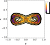 |
Fig. 6 Imagecreated by overplotting the side-on view of 12 quasi-periodic orbits around x1v2 periodic orbits at 4 different energies. The isodensity contours indicate the support of a CX-type profile. Density increases from top to bottom on the colour bar at the right of the figure. |
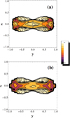 |
Fig. 7 (a) Image created by overplotting the side-on view of four sticky-chaotic orbits with initial conditions close to x1v1 periodic orbits at four different energies. (b) Same image including also four 3D quasi-periodic orbits around x1. The isodensity contours in both cases indicate the support of an OX-type profile. Density increases from top to bottom on the colour bar at the right of the figure. |
4 Comparison with the standard case
The structure of phase space we encounter in Fig. 4 can be compared with the phase space structure in a rotating Ferrers bar model, such as the one in Pfenniger (1984), Patsis et al. (2002) and similar models. In this section we compare qualitatively the phase space structure presented in Fig. 4 with that in the rotating Ferrers bar model studied by Patsis & Katsanikas (2014a).
An energy for which both 3D families of periodic orbits, which bifurcate from x1 at the vILR exist (i.e. x1v1 and x1v2) is EJ = −0.41 in the units of that model (see Patsis & Katsanikas 2014a). The projection of the space of section corresponding to Fig. 4 is given in Fig. 8. The 4D space of section in this case is (x, px, z, pz) with equations of motions derived from the Hamiltonian
 (2)
(2)
The potential Φ(x, y, z) consists of a Ferrers bar having as axisymmetric background a Miyamoto disk (Miyamoto & Nagai 1975) and a Plummer sphere (Plummer 1911). It is a typical model of a 3D strong bar. Details and numerical values of the parameters of the components of the potential, scaling of units, and so on, can be found in Patsis & Katsanikas (2014a). We note that in this case the bar is rotating counter-clockwise around the z-axis and is aligned with the y-axis. Our surface of section is defined by y = 0 and we consider the consequents with py > 0. Figures 4 and 8 have a conspicuous qualitative similarity, when rotated by 90°. Nevertheless, there is a striking difference, namely that the x1v1 and x1v2 families of periodic orbits have exchanged their stability and their relative locations. So, the location of the non-periodic orbits in phase space has changed accordingly as well.
In the configuration space, the side-on views of the quasi-periodic orbits in the tori drawn around (z, pz) = (0, 0), that is, of the 3D regular orbits around x1, are now of ∞-type, instead of having the morphology of Fig. 5a. By inspection of Fig. 8 we can see that successive projections of the tori of the 3D quasi-periodic orbits around x1, encountered as we perturb the x1 initial condition in the pz or z direction, approach the x1v2 initial condition. Their morphology now resembles that of the x1v2 periodic orbit and can be considered of similar morphology to the orbit in Fig. 5b (cf. Fig. 15e in Patsis & Katsanikas 2014a).
The quasi-periodic orbits on the tori around x1v1 and x1v1′ (on the sides of the x1 stability island in Fig. 8) support frown and smiles morphologies. They are not of ∞−type as in the case of 3D tori of Fig. 4. A set of them in the energy range in which x1v1 exists will clearly reinforce an OX peanut-shape morphology (cf. Fig. 9a in Patsis et al. 2002). On the other hand, chaotic orbits sticky to these tori, like the one plotted withthe red consequents in Fig. 8, have a hybrid character in the configuration space, in which frequently the ∞-type morphology prevails (cf. Fig. 13 in Patsis & Katsanikas 2014a). In order to obtain a basic idea of the structures that are supported by sticky-chaotic and quasi-periodic orbits in theFerrers bar model, we may look at Fig. 5b and 5c, respectively. We note that there is an overall symmetry as regards the orbital content in the two models, however, with the role of the 3D bifurcated families in providing quasi-periodic or sticky orbits being reversed.
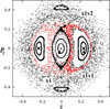 |
Fig. 8 The (z, pz) projection of the Ferrers bar model in Patsis & Katsanikas (2014a) corresponding to Fig. 4. The stability ofthe 3D families bifurcated from x1 is now reversed with respect to those of the model from the N-body simulation. Arrows indicate the locations of the main families of periodic orbits in this energy. |
5 Variation of the vertical resonances in the two models
A basic difference between the two models is the variation of their vertical frequencies. This leads to totally different “relative” energies at which the vertical resonances appear. In order to express this in a way to allow comparison of the two models, we calculate the quantity , where EJ is the energy at the location of a vertical resonance,
  is the energy of the L1 Lagrangian point and E0 is the energy at the bottom of the effective potential well, at (x, y, z) = (0, 0, 0). The relative energy, E*, gives us a measure of how close to corotation appears a vertical resonance in each model. We chose
  to represent the corotation energy, because we want to follow the behaviour of the two models along the y-axis, that is, along the major axis of the bar.
The most accurate way to locate resonances in strongly non-axisymmetric models like the two models of barred galaxies we compare, is the variation of the stability indices of their central family of periodic orbits (see e.g. Contopoulos & Grosbol 1989; Patsis & Grosbol 1996; Contopoulos 2002). In stability diagrams of axisymmetric models, the vertical stability index becomes tangent to the − 2 axis, exactly at the energies of the vertical resonances. However, in the full potential, these energies are considerably displaced from the location of the resonances in the axisymmetric background. In the presence of barred potentials, at the vertical resonances, two sets of new families of periodic orbits appear bifurcating from the bar-supporting ellipses on the plane. An example are the families bifurcated from x1 in Fig. 3, as the vertical stability index (b2 ) intersects the − 2 axis. These regions are characterised by a successive S → U → S transition of the vertical stability of the x1 family. These transitions can give us the characteristic energies at which the system “feels” the resonances.
In order to associate these energies with characteristic lengths along an axis, we need to link them with a suitable family of periodic orbits. Since we study bars, we have considered the x1 bar-supporting family on the plane and the apocentra of their orbits. In the symmetric Ferrers bar model, these apocentra, like the Lagrangian points L1 and L2, are along the major axis of the bar, while in the model from the N-body snapshot, the x1 apocentra are almost on the major axis.
We have summarised all the information for the two models we compare in Table 1. In the first column we give the n:1 vertical resonances at which the bifurcated 3D families are introduced in the system. In the second and third columns we give the quantity E*, which indicates the energy level at which a vertical resonance appears. By definition E* = 1 at  . Thus, the larger E*, the closer to corotation we have the resonant n:1 family. E* is given successively for the potential from the N-body snapshot and for the Ferrers bar model. Finally in the fourth and fifth columns we give the ratios
  for the two models, which specify the apocentra of the x1 orbits at the bifurcating energies in which the n:1 resonant 3D families are introduced. For the N-body potential
  , while in the Ferrers bar model
  .
.
There are conspicuous differences as regards the location of the, vertical resonances in the two models. In the N-body potential the two resonant 3D families associated with the 2:1 vertical resonance appear at energy levels that are more than 90% of the effective potential well height, counting from its minimum to the L1 energy (see E* column in Table 1). Contrarily, for the corresponding vertical 2:1 families of the Ferrers bar potential, E* ≈ 0.35. This means that the basic families, which in both models shape the peanut, are introduced in quite different energy levels. In order to get a better understanding of this difference, we compare the quantities  for the two models, thatis, the apocentra of the bar-supporting periodic orbits at this energy, normalized over the distance from the centre of the system to L1. In both models the apocentra and the L1, L2 Lagrangian points can be considered to be along the major axis of the bar. We observe that while in the N-body potential the peanut-supporting 3D periodic orbits start existing along the major axis of the bar at about 70% of the
  radius, in the Ferrers bar model the corresponding distance from the centre is only 12.5% of
  . In the latter case the higher-order vertical resonances 3:1 and 4:1 introduce new 3D families of periodic orbits away from the end of the bar. Their orbits are more elongated and remain closer to the equatorial plane, shaping this way a composite stair-type vertical profile (Patsis et al. 2002). This does not hold in the case of the N-body potential. We observe in Table 1 that even for the 3:1 vertical resonance, E* = 1.003, meaning that this resonance appears at an EJ between the energies of the Lagrangian points (
 ). At this energy we encounter already orbits in the bar region, which can cross corotation.
Since the vertical profiles of the bars are determined by the location of the vertical resonances and by the orbital patterns introduced by them in the system, it is clear from Table 1 that the two cases we compare are expected to be totally different in that respect. Indeed, the vertical structure of the N-body snapshot is determined almost exclusively by 3D 2:1 orbits introduced in the system very close to corotation. This leads to a fast peanut-shaped bar (corotation-to-bar ratio Rc∕Rb ≈ 1.1), in which the peanut structure is the bar itself, as we can observe in Fig. 2 (cf. also with Fig. 1 in Contopoulos & Harsoula 2013). Contrarily, the peanut of the Ferrers bar model is located in the central region of a fast bar (Rc ∕Rb ≈ 1.35), which can be composed also of orbits trapped around narrow 3D periodic orbits bifurcated at higher-order vertical n:1 resonances (n > 2) (see Fig. 12 in Patsis & Katsanikas 2014b).
The different vertical profiles of the two models could be the cause of the differences we encounter in the stability of the families of periodic orbits, which are introduced at the vertical 2:1 resonance, and consequently of the differences in the phase-space structure at the region. However, for the goals of the present study, most important is the fact that despite these differences, the vertical 2:1 resonance in both cases offers orbital building blocks that support the peanut and the X structure.
Comparison of the location of the vertical resonances in the two models along the major axis of the bar.
6 Discussion and conclusion
The case of the model from the frozen N-body snapshot we present here is rather unusual among the analytic models used so far to study the orbital dynamics in the vILR region of 3D rotating bars. Its peculiarity consists in the fact that the stable 3D families of periodic orbits introduced in the system trap around them quasi-periodic orbits that support side-on CX profiles. On the other hand, in the majority of the orbital models found in the relevant literature, the stable 3D families support side-on OX profiles as a superposition of non-periodic orbits with a frown-smile character. The stability of one or the other family and the subsequent trapping of quasi-periodic orbits around them could be the dynamical mechanism that explains the appearance of either CX or OX profiles in observed galaxies and in N-body models. However, the amount of chaos in the four-dimensional surfaces of section may play the most important role in both cases. This is indicated both in Katsanikas et al. (2013) and in Patsis & Katsanikas (2014a) and is also confirmed in the present study that presents also a different phase space structure in a vILR region. In all cases, the chaotic zone occupies a considerable volume in phase space, while it remains close to invariant tori belonging to x1 and either the stable x1v1 and x1v1′ or the set of two x1v2 orbits. Despite the fact that the surface of section has four dimensions, the presence of these tori close to each other (Figs. 4 and 8) create zones of stickiness that are able to keep the particles in the region for times of the order of several Gyr and thus bring into the system orbits that can support structures within this time period1. Several papers use two-dimensional frequency analysis in order to classify the observed orbital morphologies (see e.g. Ceverino & Klypin 2007; Voglis et al. 2007; Harsoula & Kalapotharakos 2009; Valuri et al. 2016; Wang et al. 2016; Abbot et al. 2017). However, in the presence of sticky (weakly chaotic) orbits, it is difficult to attribute the observed structure to a specific 3D resonant family of periodic orbits. Hybrid morphologies will be present and a detailed investigation of the phase space structure is needed in order to identify the prevailing contribution by one of them.
Both CX and OX profiles can be built by orbits introduced in the vILR resonance of the two models. The existence of vertical resonances is not a particular property of a model. Vertical resonances exist in 3D rotating potentials and the vertical 2:1 resonance is a basic one. By investigating the conditions under which a CX or OX profile will be formed, we realise that by populating the model with sticky orbits together with the 3D quasi-periodic orbits trapped in the neighbourhood of x1, one can create a profile based on the presence of the unstable periodic orbits, instead of the one expected by the prevalence of the quasi-periodic orbits of the stable 3D family in each case. Thus, the model of the frozen snapshot of the N-body model of Contopoulos & Harsoula (2013) can build a CX profile by means of quasi-periodic orbits around the stable x1v2 periodic orbit and an OX profile using the quasi-periodic orbits around x1 combined with the sticky chaotic orbits emanating from the neighbourhood of the unstable x1v1. On the other hand, in the standard case of a rotating Ferrers bar, like the one in Patsis & Katsanikas (2014a), the role of quasi-periodic and chaotic orbits associated with the x1v1 and x1v2 is reversed. However, both models provide the building blocks for each type of profile. The present study underlines the flexibility that exists in dynamical mechanisms, which are based on 3D orbits “born” at the vILR of a rotating bar, in supporting boxy/peanut-shaped bulges.
In summary:
-
In the standard case regular orbits support OX profiles and sticky chaotic CX ones.
-
In cases like the potential from the Contopoulos & Harsoula (2013) model, sticky chaotic orbits support OX profiles and regular orbits CX ones. This is valid also for the energies in which the x1v2 family becomes stable, while x1v1 is unstable, in any model.
-
It is the chaoticity of the profiles that decides which dynamical mechanism will prevail. Definitely, in both cases the vILR region provides dynamical mechanisms for building X-shaped central regions in barred galaxy models.
Acknowledgements
This work was partly supported by the Research Committee of the Academy of Athens, project number 200/854. We acknowledge fruitful discussions with G. Contopoulos and L. Athanassoula.
References
- Abbott, C. G., Valluri, M., Shen, J., & Debattista, V. P. 2017, MNRAS, 470, 1526 [NASA ADS] [CrossRef] [Google Scholar]
- Allen, A. J., Palmer, P. L., & Papaloizou, J. 1990, MNRAS, 242, 576 [NASA ADS] [CrossRef] [Google Scholar]
- Athanassoula, E., & Misiriotis, A. 2002, MNRAS, 330, 35 [NASA ADS] [CrossRef] [Google Scholar]
- Broucke, R. 1969, NASA Techn. Rep., 32, 1360 [Google Scholar]
- Bureau, M., Aronica, G., Athanassoula, E., et al. 2006, MNRAS, 370, 753 [NASA ADS] [CrossRef] [Google Scholar]
- Ceverino, D., & Klypin A. 2007, MNRAS, 379, 1155 [NASA ADS] [CrossRef] [Google Scholar]
- Combes, F., Debbasch, F., Friedli, D., & Pfenniger, D. 1990, A&A, 233, 82 [NASA ADS] [Google Scholar]
- Contopoulos, G. 2016, Order and chaos in dynamical astronomy (Berlin: Springer) [Google Scholar]
- Contopoulos, G., & Magnenat, P. 1985, Celest. Mech., 37, 387 [NASA ADS] [CrossRef] [Google Scholar]
- Contopoulos, G., & Grosbol, P. 1989, A&ARv, 1, 261 [NASA ADS] [CrossRef] [Google Scholar]
- Contopoulos, G., & Harsoula, M. 2013, MNRAS, 436, 1201 [NASA ADS] [CrossRef] [Google Scholar]
- Ferrers, N. M. 1870, R. Soc. London Phil. Trans. Ser. I, 160, 1 [NASA ADS] [CrossRef] [Google Scholar]
- Harsoula, M., & Kalapotharakos, C. 2009, MNRAS, 394, 1605 [NASA ADS] [CrossRef] [Google Scholar]
- Katsanikas, M., & Patsis, P. A. 2011, Int. J. Bif. Chaos, 21, 467 [CrossRef] [Google Scholar]
- Katsanikas, M., Patsis, P. A., & Contopoulos, G. 2013, Int. J. Bif. Chaos, 23, 1330005 [CrossRef] [Google Scholar]
- Miyamoto, M., & Nagai, R. 1975, PASJ, 27, 533 [NASA ADS] [Google Scholar]
- Mulder, W. A., & Hooimeyer, J. R. A. 1984, A&A, 134, 158 [NASA ADS] [Google Scholar]
- Patsis, P. A., & Zachilas, L. 1994, Int. J. Bif. Chaos, 4, 1399 [CrossRef] [Google Scholar]
- Patsis, P. A., & Grosbol, P. 1996, A&A, 315, 371 [NASA ADS] [Google Scholar]
- Patsis, P. A., & Katsanikas, M. 2014a, MNRAS, 445, 3525 [NASA ADS] [CrossRef] [Google Scholar]
- Patsis, P. A., & Katsanikas, M. 2014b, MNRAS, 445, 3546 [NASA ADS] [CrossRef] [Google Scholar]
- Patsis, P. A., Skokos, Ch., & Athanassoula, E. 2002, MNRAS, 337, 578 [NASA ADS] [CrossRef] [Google Scholar]
- Pfenniger, D. 1984, A&A, 134, 373 [NASA ADS] [Google Scholar]
- Pfenniger, D., & Friedli, D. 1991, A&A, 252, 75 [NASA ADS] [Google Scholar]
- Plummer, H. C. 1911, MNRAS, 71, 460 [CrossRef] [Google Scholar]
- Skokos, Ch., Patsis, P. A., & Athanassoula, E. 2002, MNRAS, 333, 847 [NASA ADS] [CrossRef] [Google Scholar]
- Tsoutsis, P., Efthymiopoulos, C., & Voglis, N. 2008, MNRAS, 387, 1264 [NASA ADS] [CrossRef] [Google Scholar]
- Valluri, M., Shen, J., Abbott, C., & Debattista, V. P. 2016, ApJ, 818, 141 [NASA ADS] [CrossRef] [Google Scholar]
- Voglis, N., Harsoula, M., & Contopoulos, G. 2007, MNRAS, 381, 757 [NASA ADS] [CrossRef] [Google Scholar]
- Wang, Y., Athanassoula, E., & Mao, S. 2016, MNRAS, 463, 3499 [NASA ADS] [CrossRef] [Google Scholar]
We note that in the 3D Ferrers bar model there is one more set of stable tori, as we can observe in the upper and lower part of Fig. 8 for z = 0, that has its own sticky zone of influence (consequents in the periphery of the chaotic region that surrounds the stability islands) and gives a third alternative for a side-on morphology – see Patsis & Katsanikas (2014a). However, we do not discuss this case in the present study.
All Tables
Comparison of the location of the vertical resonances in the two models along the major axis of the bar.
All Figures
|
Fig. 1 A sketch of the two types of X features appearing in edge-on views of disk galaxies: (a) The CX type, in which the wings of theX cross the centre of the system, and (b) the OX profile, in which the wings of X avoid the centre. |
| In the text | |
|
Fig. 2 (a) The side-on profile of the N-body model. (b) The side-on profile consisting of orbits belonging to the 2:1 class in the corresponding frozen potential (Contopoulos & Harsoula 2013). The plotted isodensities in (b) emphasise the CX character of the profile. L1 and L2 indicate the location of the unstable Lagrangian points. Darker colour corresponds to more dense regions. |
| In the text | |
|
Fig. 3 Evolution of the stability indices of the main families at the vILR region. From the mother family x1, bifurcate first the x1v2 as stable and second the x1v1 as unstable. |
| In the text | |
|
Fig. 4 (z, ż) projection of the space of section for the main orbits that participate in building the side-on profile of the model, for EJ = − 1.15×10⁶. Heavy dots indicate the location of x1v1 and x1v2, while the x1 periodic orbit is projected at (z, ż ) ≈ (0, 0). Arrows point to the initial conditions of the orbits given in Fig. 5. |
| In the text | |
|
Fig. 5 (a) The 3D quasi-periodic orbit around x1 indicated with “a” in Fig. 4. (b) The quasi-periodic orbit around x1v2indicated with “b” in Fig. 4. (c) The sticky chaotic orbit corresponding to the scattered green consequents in the chaotic zone of the same figure. All orbits have been integrated for time giving 30 consequents on the y = 0 space of section with ẏ < 0. |
| In the text | |
|
Fig. 6 Imagecreated by overplotting the side-on view of 12 quasi-periodic orbits around x1v2 periodic orbits at 4 different energies. The isodensity contours indicate the support of a CX-type profile. Density increases from top to bottom on the colour bar at the right of the figure. |
| In the text | |
|
Fig. 7 (a) Image created by overplotting the side-on view of four sticky-chaotic orbits with initial conditions close to x1v1 periodic orbits at four different energies. (b) Same image including also four 3D quasi-periodic orbits around x1. The isodensity contours in both cases indicate the support of an OX-type profile. Density increases from top to bottom on the colour bar at the right of the figure. |
| In the text | |
|
Fig. 8 The (z, pz) projection of the Ferrers bar model in Patsis & Katsanikas (2014a) corresponding to Fig. 4. The stability ofthe 3D families bifurcated from x1 is now reversed with respect to those of the model from the N-body simulation. Arrows indicate the locations of the main families of periodic orbits in this energy. |
| In the text | |
Current usage metrics show cumulative count of Article Views (full-text article views including HTML views, PDF and ePub downloads, according to the available data) and Abstracts Views on Vision4Press platform.
Data correspond to usage on the plateform after 2015. The current usage metrics is available 48-96 hours after online publication and is updated daily on week days.
Initial download of the metrics may take a while.