| Issue |
A&A
Volume 611, March 2018
|
|
|---|---|---|
| Article Number | A73 | |
| Number of page(s) | 8 | |
| Section | Planets and planetary systems | |
| DOI | https://doi.org/10.1051/0004-6361/201731502 | |
| Published online | 29 March 2018 | |
Stability criteria for wide binary stars harboring Oort Clouds
Grupo de Ciencias Planetarias, Departamento de Geofísica y Astronomía, Facultad de Ciencias Exactas, Físicas y Naturales, Universidad Nacional de San Juan – CONICET. Av. J. I. de la Roza 590 oeste, J5402DCS Rivadavia, San Juan, Argentina
e-mail: This email address is being protected from spambots. You need JavaScript enabled to view it.
Received:
3
July
2017
Accepted:
28
November
2017
Abstract
Context. In recent years, several numerical studies have been done in the field of the stability limit. Although, many of them included the analysis of asteroids or planets, is not possible to find in the literature any work on how the presence of a binary star could affect other possible configurations in a three-body problem. In order to develop this subject we consider other structures like Oort Clouds in wide binary systems. Regarding the existence of Oort Clouds in extrasolar systems there are recent works that do not reject its possible existence.
Aim. The aim of this work is to obtain the stability limit for Oort Cloud objects considering different masses of the secondary star and zero and non-zero inclinations of the particles. We improve our numerical treatment getting a mathematical fit that allows us to find the limit and compare our results with other previous works in the field.
Methods. We use a symplectic integrator to integrate binary systems where the primary star is m1 = 1 M⊙ and the secondary, m2, takes 0.25 M⊙ and 0.66 M⊙ in two sets of simulations S1 and S2. The orbital parameters of the secondary star were varied in order to study different scenarios. We also used two different integration times (one shorter than the other) and included the presence of 1000 to 10 000 massless particles in circular orbits to form the Oort Cloud. The particles were disposed in four different inclination planes to investigate how the presence of the binary companion could affect the stability limit.
Results. Using the Maximum Eccentricity Method, emax, together with the critical semimajor axis acrit we found that the emax criteria could reduce the integration times to find the limit. For those cases where the particles were in inclined orbits we found that there are particle groups that survive the integration time with a high eccentricity. These particle groups are found for our two sets of simulations, meaning that they are independent of the secondary mass. We also find for the co-planar case that the numerical value of the stability limit for retrograde orbits is higher than those found for prograde orbits. These results are in agreement with several published studies. Finally, the results obtained in this work allow us to build a numerical expression depending of the mass ratio, e2 and ip to find acrit, which can be compared with other recent works in the field.
Key words: methods: numerical / Oort Cloud / binaries: general / planets and satellites: dynamical evolution and stability
© ESO 2018
1 Introduction
Since the discovery of the first exoplanetary system, 51 Peg b by Mayor & Queloz (1995), it is evident that planets do not form only around single stars, but can also be present in multiple-stars systems in a variety of different configurations (Roell et al. 2012). One simple but important question related to the exoplanetary systems is in regards to the locations in which planets can be found if the star is binary. A detailed study of the stability of the planetary orbits could reveal these locations.
The stability criteria have been studied by many authors. For example, Szebehely (1967) and Henon (1970) used analytical models to analyze coplanar systems, finding that the most stable orbits were retrograde. Later, Innanen (1979, 1980) improved on this by considering arbitrary inclinations. Nevertheless, all these works were analytical approaches to the stability limit and it was necessary to wait until a decade later when several numerical studies of the stability limit were carried out (Hamilton & Burns 1991; Wiegert & Holman 1997; Holman & Wiegert 1999) and showed significant differences with the previous analytical results. While the analytical work of Innanen (1979, 1980) found that the radius is an increasing function of the inclination, Hamilton & Burns (1991) showed numerically that the radius starts to decreases at ~60° and increases at higher inclinations.
This discrepancy between analytical and numerical results was recently studied by Grishin et al. (2017) in the framework of the three-body problem. They used the Hill-stability criteria coupled with a Lidov-Kozai mechanism (Lidov 1962; Kozai 1962) for the inclined case. It is worth mentioning that in the work of Grishin et al. (2017), a mass hierarchical system is used, where the more distant object is also the more massive. They also found a polynomial fit for their results, as many other authors have done in the past.
On the other hand, considering the amount of planets found in binary configurations and the recent concern about harboring extrasolar Oort Clouds (Nordlander et al. 2017), the formation of such structures in binary systems seems possible. Hence, it could be interesting to extend the study of the stability limit to wide binaries (those systems with separations > 1000 au) harboring Oort Clouds.
In the case of the solar system, the Oort Cloud was studied by several authors (for a more detailed review of the Oort Cloud formation we refer the reader to Dones et al. 2015). Some works included galactic perturbations (Heisler & Tremaine 1986), flyby of passing stars (Oort 1950), encounters with molecular clouds (e.g., Hut & Tremaine 1985; Jakubík & Neslušan 2009) and formation in clusters (e.g., Fernández & Brunini 2000; Brasser et al. 2006; Kaib & Quinn 2008; Brasser & Morbidelli 2013), However, we do not find in the literature any work that explores thepossibility of finding this kind of particle system in binaries or anyone that has studied its stability limit.
In this paper we study the stability limit for an Oort Cloud in a wide binary system, using massless particles with orbits in different planes and not only in the plane of the binary. We also used a range of masses for the binary components and a range of eccentricities for their orbits to decipher whether or not the presence of a binary companion could affect the cloud. We describe the method used to make the simulations in Sect. 2. In Sect. 3 we discuss the results and we summarize the conclusions in Sect. 4.
2 Methods
To carry out the study of the stability limit of test particles in binary systems we used a symplectic integrator based on the code proposed by Chambers et al. (2002). We simulate a spherical Oort Cloud surrounding the primary star of the binary with mass m1 = 1M⊙. To test different configurations, we change the eccentricity of the orbit and the mass ratio μ = m2∕(m1 + m2), where m2 is the secondary mass. This choice was motivated by the fact that the vast majority of exoplanets found in wide binaries are orbiting the most massive star 1.
We carry out two sets of simulations (thereafter S1 and S2), with four values of the binary eccentricity, 0.2, 0.4, 0.6 and 0.8. The inclinations are taken from the plane of the binary, considered as the reference plane.
In our S1 simulation we integrate 1000 binary periods, and the value of the secondary mass was m2 = 0.25 M⊙, or μ = 0.2. On the other hand, in the S2 simulation we integrate 10 000 binary periods for m2 = 0.66 M⊙, or μ = 0.4. For each set of simulations we used two different values for the semimajor axis of the binary, but we rescale the unit length in order to compare our results with other authors. For that purpose we state our results using α = ap∕a2 so that α < 1.
The initial orbit for all the particles was circular and different inclinations were considered, thus we checked the stability limit for those cases where the particles are in the orbital plane of the stars, that is ib = 0°, and also for inclinations of 60°, 120° and 180°. The rest of the orbital elements of the binary and particles were chosen randomly. All the relevant orbital parameters are listed in Table 1. Then, we follow the temporal evolution of 10 000 particles (set S1) and 1000 particles (set S2 ) for each combinationof e2 and ip, which leads to a total of 160 000 and 16 000 particles for the first and second sets, respectively. It is worth noting that the most internal particles complete more than 106 orbits around m1 in the total time of the integration.
Because we are using a symplectic integrator, we defined a fixed integration step of one tenth of the period of the most inner particle. In the case where a particle approaches the central star (m1 ) at a distance of less than a half of the initial distance of the inner particle, it is discarded.
To determine the stability limit, we follow the criteria of Holman & Wiegert (1999), which are based on the evolution life time of the test particles. However, weuse the emax method to reduce the integration time and improve the computing capacity. The Maximum EccentricityMethod (MEM; Dvorak et al. 2004 looks for the maximum value of eccentricity (emax) attained by a test particle during the numerical simulation and becomes a useful tool to predict the instability of the orbits. In this method a massless particle that reaches emax ≥ 1 is discarded because we consider that it has escaped the gravitational potential of the primary star m1 . Therefore, we consider the stability limit to be the smallest value of α for which the particles achieve emax = 1.
We apply the MEM method to our two sets S1 and S2. In the case of S2 we use our simulation to numerically test the method, although previous works (for example Ramos et al. 2015) have shown that this method is effective in stability studies for the restricted three-body problem (see Sect. 3.1). It is worth noting that surviving test particles with emax < 1 could be found beyond the stability limit (specially in the case S1), but the MEM predicts that such particles become unstable, which is confirmed in our numerical test, as we show in Sect. 3.1.
Initial conditions for the two sets of simulations performed.
3 Results
We separatethe results into two cases: “zero inclination” and “non-zero inclination”. For both cases, we plot emax against α, which depends on the initial semimajor axis of the particle. We use α to compare our results with Holman & Wiegert (1999) who define the value of acrit as the initial semimajor axis at which the test particles at any longitude survive the full integration time. The results from this and analyses from the following section are listed in Table 2.
Numerical results for the two sets of simulations performed.
3.1 Zero-inclination results
Figure 1 shows our results for ip = 0°. In each panel we plot our two sets of simulations for the intervals of eccentricities considered. It is possible to see that the behavior of the particles is similar for the two sets and in the case of μ = 0.4 the particles become unstable at smaller values of α. To obtain the value of the stability limit in this case, we used the same criteria of Holman & Wiegert (1999), implying that the behavior of the particles is independent of the binary eccentricity and the secondary mass.
The values obtained for the zero-inclination case (listed in Table 2) are very similar to those found by Holman & Wiegert (1999). To see how similar they are we compare them in Figs. 2 and 3. The error bars were calculated from the Δa of the simulated particles, which is the same criteria used by Holman & Wiegert (1999). It can be seen that our results are similar to those found previously by these authors, although the error bars in our work are much smaller, even considering that we used the same procedure. However, the main difference between our work and that of Holman & Wiegert (1999) is the longer integration time used. Holman & Wiegert (1999) compared their results with that of Rabl & Dvorak (1988) who used only 300 binary periods, concluding that a number of 10 000 binary periods is a short time to find the stability limit. Then, taking into account the ages of binary systems they infer that it is important to consider much longer integration times to see if other instabilitiesappear. In a recent paper, Ramos et al. (2015) proposed even longer integration times such as 105 binary periods.
As mentioned above, the emax criteria is useful for finding the value of the critical semimajor axis. We use the simulations of our set S2 to numerically test the MEM. The 1000 test particles of the 16 simulations are evolved by the total integration time (i.e., 10 000 binary periods), and we also save the maximum value of the eccentricity for each particle in each output of our simulation. To show how the emax method could help to reduce the integration times, in Fig. 4 we plot the results of one planar case for the set S2 . We show the output for three different binary periods for e2 = 0.6. It is possibleto see that in 300 binary orbits those particles with α greater thanthat of the first particle to achieve an eccentricity value of 1 become unstable at the end of the simulation. The same happens for 1000 binary orbits, but the first particle with emax = 1 is next to the surviving stability limit defined for 10 000 binary orbits. As we will show in the next section we found the same result for the retrograde and non-planar cases. Therefore, this led us to deduce that it is possible to work with just 1000 binary orbits and put the limit in the minimum value of α for which the particles reach emax = 1. We apply this criteria for our set S1.
In addition to Fig. 4 we plot in Fig. 5 the percentage of particles that reach a stable or unstable orbit for the same set used in Fig. 4. We included only the first 1000 binary periods because the variation in the percentage from 1000 to 10 000 periods is very small( ~ 1%) and does not have a strong influence on the stability limit. In this case, the most important change in the number of the surviving particles is produced between 100 and 300 periods where it decreases by 1.6%, while for the period between 300 and 1000 binary periods the variation is even lower (1.4%).
Applying the emax criteria to our set S1 we found similar results to those found by Holman & Wiegert (1999), as we show in Fig. 2. Then, we can conclude that using the emax criteria we can significantly reduce the integration time needed to determine the stability limits of the system.
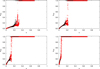 |
Fig. 1 Comparison between the results found in the “Zero inclination case” for different values of e2 . We compare our two sets of simulations S1 and S2 for μ = 0.2 (red plot) and μ = 0.4 (black plot), respectively. Top-left, top-right, bottom-left and bottom-right panels correspond to the values of e2 = 0.2, 0.4, 0.6 and 0.8, respectively. |
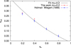 |
Fig. 2 Comparison between the results found in this work and Holman & Wiegert (1999) for μ = 0.2. The red plot corresponds to this work and the blue one was taken from Holman & Wiegert (1999) for different eccentricities of the binary (e2). |
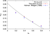 |
Fig. 3 Comparison between the results found in this work and Holman & Wiegert (1999) for μ = 0.4. The red plot corresponds to this work and the blue one was taken from Holman & Wiegert (1999) for different eccentricities of the binary (e2). |
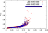 |
Fig. 4 Value of α against emax for three different binary periods for the same mass and binary eccentricity. In this case ip = 0° and the parameters of the secondary are e2 = 0.6 and m2 = 0.66. It can be seen that the difference between the critical semimajor axis when the particles become unstable is not significantly different between 300 (red plot), 1000 (black plot) and 10 000 binary periods (blue plot). |
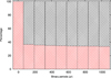 |
Fig. 5 Stability percentage for ip = 0°, e2 = 0.6 and m2 = 0.66 from 0 to 1000 binary periods. The red and black histograms correspond to the stable and unstable particles, respectively. |
3.2 Non-zero inclination results
In Figs. 6 to 8, emax is plotted against α for the other inclination planes (ip = 60°, ip = 120° and ip = 180°), in which the two cases S1 and S2 are shown in red and black, respectively. For retrograde orbits (Fig. 8) we found a result similar to that of ip = 0° (Fig. 1), where the maximum of eccentricity increases slowly with the increase of α and we can see the presence of some mean motion resonances of high order.
In Figs. 6 and 7 it is possible to see a region of high eccentricity where all the massless particles have emax ≥ 0.75. The dynamical behavior that produces this increase in eccentricity is the Lidov-Kozai mechanism (LK) studied by Lidov (1962) and Kozai (1962) in the framework of the restricted three-body problem (RTBP). The LK mechanism has been described in the literature in great detail and the reader is referred to Naoz (2016) for a review of the mechanism, recent developments and its applications.
In the Lidov-Kozai mechanism, there is a time scale associated to the oscillations of the eccentricity and inclination, which has been explored by Grishin et al. (2017) for the case of a general three-body problem. The approximation of the LK cycle for the case of a restricted three-body problem is:
![Mathematical equation: $T_{LK} \approx \frac{\sqrt{1-\mu}}{\mu} \left[ \dfrac{1-e_{2}^2}{\alpha} \right] ^{3/2} P_{2} \textrm{,} $](/articles/aa/full_html/2018/03/aa31502-17/aa31502-17-eq1.png) (1)
(1)
with P2 being the binary period.
As we set TKL as a function of the binary period P2, we can compare this expression with the criteria of Holman & Wiegert (1999). It is possible to see that the LK time scale is inversely proportionalto α and consequently to the semimajor axis of the massless particle, therefore we can estimate for our numerical results the limit for the initial conditions that complete a LK cycle. Then, for the S1 simulation which has a total integration time of 1000P2, the limit in α for the complete LK cycle is between 0.025 and 0.009, being e2 = 0.2 and e2 = 0.8, respectively. For the S2 simulation (in this case the total integration time is 10 000P2) the limit of α is 0.0032 considering e2 = 0.2, and 0.0012 for e2 = 0.8.
For massless particles with initial circular orbits, the maximum eccentricity attained during a LK cycle could be found from the conservation of the component z of the angular momentum; considering a minimum inclination of 39.2° (Grishin et al. 2017) we find:
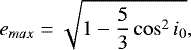 (2)
(2)
where i0 is the initial value of inclination. This value is independent of the masses of the binary system and the orbit of m2 , thus for massless particles out of the plane (i.e., ip = 60° and 120°) we obtain an emax ~ 0.76. It is worth mentioning that, as Grishin et al. (2017) shows, the minimum inclination depends on the semimajor axis (see Eq. (14) of Grishin et al. (2017)). Therefore, in our results we obtain a value for maximum eccentricity that is not constant, but it also depends on the semimajor axis.
From Figs. 6 and 7 it is possible to confirm the theoretical predictions of the LK mechanism in our numerical results. There is a group of massless particles with small values of α and emax, which correspond to the case of particles that do not complete the LK cycle during the simulation. Moreover, in all cases, the maximum eccentricity of the stable particles depends on the semimajor axis. An increase of emax is seen with the increase of a , confirming the results of Grishin et al. (2017) that we mention above.
As a comparison with Fig. 5 for the ip = 0° case, the percentage of particles that reach a stable or unstable orbit with ip = 60° in the first 1000 binary periods is shown in Fig. 9, where it is also possible to observe a 3.2% change in the number of the survivor particles produced between 100 and 300 periods, while for the period between 300 and 1000 binary periods the variation is 2.6%. Although the comparison between inclinations shows that more particles became unstable at the beginning of the integration for ip = 0°, the general behavior for both groups is the same: in the first 300 binary periods there are more particles becoming unstable than in the rest of the integration.
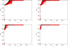 |
Fig. 6 Comparison between the results found for ip = 60°. We compare our two sets of simulations S1 and S2 for μ = 0.2 (red plot) and μ = 0.4 (black plot), respectively. Each panel corresponds to a different value of e2. Top-left, top-right, bottom-left and bottom-right panels correspond to the values of e2 = 0.2, 0.4, 0.6 and 0.8, respectively. |
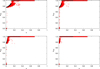 |
Fig. 7 Comparison between the results found for ip = 120°. We compare our two sets of simulations S1 and S2 for μ = 0.2 (red plot) and μ = 0.4 (black plot), respectively. Each panel corresponds to a different value of e2. Top-left, top-right, bottom-left and bottom-right panels correspond to the values of e2 = 0.2, 0.4, 0.6 and 0.8, respectively. |
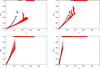 |
Fig. 8 Comparison between the results found for ip = 180°. We compare our two sets of simulations S1 and S2 for μ = 0.2 (red plot) and μ = 0.4 (black plot), respectively. Each panel corresponds to a different value of e2. Top-left, top-right, bottom-left and bottom-right panels correspond to the values of e2 = 0.2, 0.4, 0.6 and 0.8, respectively. |
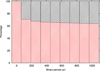 |
Fig. 9 Stability percentage for ip = 60°, e2 = 0.6 and m2= 0.66 from 0 to 1000 binary periods. The red and black histograms correspond to the stable and unstable particles, respectively. |
3.3 Polynomial fit
Using the stability limits found for the different cases considered, we made a least-squares fit to obtain an expression that gives the value of acrit as a function of e2, μ and θ = cosip. We used a polynomial of third degree in these variables and the best fit found is:
![Mathematical equation: \begin{align} a_{crit} & = &[c_{0}+c_{1} e_{2}+c_{2} \mu +c_{3} \theta +c_{4} e_{2}^2+c_{5} \mu^2 +c_{6} \theta^2 \\ & & +c_{7} e_2 \mu +c_{8} e_{2} \theta +c_{9} \mu \theta+c_{10} e_{2}^3+c_{11} \mu^3 +c_{12} \theta^3 \\ & & +c_{13} e_{2}^2 \mu +c_{14} e_{2}^2 \theta +c_{15} \mu^2 e_{2}+c_{16} \mu^2 \theta \\ & &+c_{17} \theta^2 e_{2} +c_{18} \theta^2 \mu +c_{19} e_{2} \mu \theta ]a_{2}\,\textrm{,}\end{align}](/articles/aa/full_html/2018/03/aa31502-17/aa31502-17-eq3.png) (3)
(3)
where each one of the coefficients ci is listed in Table 3.
The polynomial fit found is indicated with a black solid line in Figs. 2 and 3 for comparison . It is possible to see that the black line fits the points very accurately, not only for our results, but also for those obtained by Holman & Wiegert (1999). As an example of a case with an inclination different from zero, we plot the best fit for ip = 180° in Fig. 10; however, we find a very good agreement for all the other values of ip considered.
One important result arising from the comparison of the stability limit found for ip = 60° and ip = 120° is that the value in the last case is slightly lower than that of the first one, which does not contradict the results found by other authors since the most stable orbits are those that are retrograde (Szebehely 1967; Henon 1970; Gayon & Bois 2008; Morais & Giuppone 2012). To explain this behavior we plot in Fig. 11 the intersection of the polynomial fit and the plane i vs. acrit for e2 = 0.4, where the results for μ = 0.2 and 0.4 are indicated with blue stars and black boxes, respectively. In this Figure the value of the stability limit can be seen to change as a function of the inclination: the critical semimajor axis reduces its value to a minimum and then it increases to reach a maximum value. Comparing the cases of ip = 0° and ip = 180°, the higher value for acrit is obtained for the retrograde orbit, but this is not necessarily fulfilled when other pairs of prograde-retrograde orbits are compared (for example ip = 60° and ip = 120°). It is also important to note that this behavior of the inclination is also seen for other values of e2 .
Figure 11 shows us that the lowest critical semimajor axis is found when the inclination is close to ip = 90° and its maximum value is close to ip = 180°. This impliesthat for those particles with orbits in planes perpendicular to the reference plane, the critical semimajor axis is lower than for those particles orbiting near the reference plane. This leads us to propose that the binary companion in this kind of system could affect the shape of the particle cloud and that its shape could more closely resemble an ellipsoidal figure than a sphere.
Moreover, our results are similar to those of Grishin et al. (2017), who analyzed a generalized Hill stability criteria for hierarchical three-body systems. If we compare our Fig. 11 with the circular grid of Grishin (2017; see their Fig. 6), it is possibleto see a similar dependence of the stability limit on the inclination. In their Fig. 6 there is a minimum near to i ~ 90° and a maximum at i = 180°, which is also observed in our Fig. 11, but there is also a difference near i = 60°, where the stability limit is greater than i = 0°. We think that this difference is probably produced by the inclination sampling, because we only considered four values for ip , but in general terms the dependence with inclination is well represented by our fit.
Despite the similarity between our work and Grishin et al. (2017), an important difference between them is worth noting: we use a mass ratio m1 ∕m2 > 0.1 while Grishin et al. (2017) used a m1∕m2 ~ 10−6, which means that there are several orders of magnitude between these two values, putting each one of these works in different regimes (Holman & Wiegert 1999). Our results allow us to make a linear approximation of the dependence of the limit on the mass ratio, while Grishin et al. (2017) mostly focused on the inclination and not on the mass ratio.
Coefficients of our numerical fit.
 |
Fig. 10 Polynomial fit for ip = 180°. Black plot corresponds to the fit for μ = 0.2 and the blue one to the fit for μ = 0.4. The red stars and the black squares are the results of our work for μ = 0.2 and μ = 0.4, respectively. |
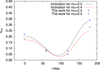 |
Fig. 11 Variation of the critical semimajor axis with the ip for e2 = 0.4. Plotted are the results found in this work for ip = 0°, 60°, 120° and 180° of our two sets of simulations. The black and red lines correspond to the polynomial fit. |
4 Conclusions
In this paper we have developed a stability criteria for an Oort Cloud around wide binary systems considering the cases of ip ≥ 0°.
We used the same approximation of Holman & Wiegert (1999) to find the stability limit, except that we introduce the use of emax, which is a chaos indicator that tell us the maximum value of e attained bya particle through a numerical simulation. For the case ip = 0° the stabilitylimit obtained with our method is quite similar to Holman & Wiegert (1999) and the main differencewith our result is the integration time used to determine the stability limit. We concluded that the emax method could help us to reduce the integration times used.
From the non-zero inclination cases we find that the particles inclined by 60° and 120° show a region of high emax for values of α near to acrit. This increase of the eccentricity values is present in all our integrations for ip = 60° and ip = 120° and different m2 masses, making our results independent of the parameters of the secondary star. From previous studies (i.e., Grishin et al. 2017) we determine that the Lidov-Kozai resonance is responsible for the behavior in this region, and those particles at values of α that did not reach the theoretical value of emax are the consequence of not having enough time to evolve and be scattered.
We also make a least squares fit for μ, e2 and ip , finding thatit fits very well to our results and to those of Holman & Wiegert (1999) for ip = 0°. Further, we test the fit for ip > 0° , also finding a very good agreement.
Finally, using the variation of acrit for the different values of ip , it is possible to see that the critical semimajor axis reduces its value to a minimum for ip = 90° and then it increases to a maximum close to ip = 180°. This result could imply that the presence of a binary companion could affect the shape of an Oort Cloud around the main star and such structures could have shapes more closely resembling an ellipsoidal than a sphere.
Acknowledgements
The authors gratefully acknowledge financial support from CONICET through PIP 112-201501-00525.
References
- Brasser, R. & Morbidelli, A. 2013, Icarus, 225, 40 [NASA ADS] [CrossRef] [Google Scholar]
- Brasser, R., Duncan, M. J., & Levison, H. F. 2006, Icarus, 184, 59 [NASA ADS] [CrossRef] [Google Scholar]
- Chambers, J. E., Quintana, E. V., Duncan, M. J., & Lissauer, J. J. 2002, AJ, 123, 2884 [NASA ADS] [CrossRef] [Google Scholar]
- Dones, L., Brasser, R., Kaib, N., & Rickman, H. 2015, Space Sci. Rev., 197, 191 [NASA ADS] [CrossRef] [Google Scholar]
- Dvorak, R., Pilat-Lohinger, E., Schwarz, R., & Freistetter, F. 2004, A&A, 426, L37 [NASA ADS] [CrossRef] [EDP Sciences] [Google Scholar]
- Fernández, J. A. & Brunini, A. 2000, Icarus, 145, 580 [NASA ADS] [CrossRef] [Google Scholar]
- Gayon, J. & Bois, E. 2008, in Exoplanets: Detection, Formation and Dynamics, ed. Y.-S. Sun, S. Ferraz-Mello, & J.-L. Zhou, IAU Symposium, 249, 511 [NASA ADS] [Google Scholar]
- Grishin, E., Perets, H. B., Zenati, Y., & Michaely, E. 2017, MNRAS, 466, 276 [NASA ADS] [CrossRef] [Google Scholar]
- Hamilton, D. P. & Burns, J. A. 1991, Icarus, 92, 118 [NASA ADS] [CrossRef] [Google Scholar]
- Heisler, J. & Tremaine, S. 1986, Icarus, 65, 13 [NASA ADS] [CrossRef] [Google Scholar]
- Henon, M. 1970, A&A, 9, 24 [NASA ADS] [Google Scholar]
- Holman, M. J. & Wiegert, P. A. 1999, AJ, 117, 621 [NASA ADS] [CrossRef] [Google Scholar]
- Hut, P. & Tremaine, S. 1985, AJ, 90, 1548 [NASA ADS] [CrossRef] [Google Scholar]
- Innanen, K. A. 1979, AJ, 84, 960 [NASA ADS] [CrossRef] [Google Scholar]
- Innanen, K. A. 1980, AJ, 85, 81 [NASA ADS] [CrossRef] [Google Scholar]
- Jakubík, M. & Neslušan L. 2009, Contrib. Astron. Obs. Skaln. Pleso, 39, 85 [NASA ADS] [Google Scholar]
- Kaib, N. A. & Quinn, T. 2008, Icarus, 197, 221 [NASA ADS] [CrossRef] [Google Scholar]
- Kozai, Y. 1962, AJ, 67, 591 [Google Scholar]
- Lidov, M. L. 1962, Planet. Space Sci., 9, 719 [NASA ADS] [CrossRef] [Google Scholar]
- Mayor, M. & Queloz, D. 1995, Nature, 378, 355 [NASA ADS] [CrossRef] [Google Scholar]
- Morais, M. H. M. & Giuppone, C. A. 2012, MNRAS, 424, 52 [NASA ADS] [CrossRef] [Google Scholar]
- Naoz, S. 2016, ARA&A, 54, 441 [Google Scholar]
- Nordlander, T., Rickman, H., & Gustafsson, B. 2017, A&A, 603, A112 [NASA ADS] [CrossRef] [EDP Sciences] [Google Scholar]
- Oort, J. H. 1950, Bull. Astron. Inst. Netherlands, 11, 91 [Google Scholar]
- Rabl, G. & Dvorak, R. 1988, A&A, 191, 385 [NASA ADS] [Google Scholar]
- Ramos, X. S., Correa-Otto, J. A., & Beaugé, C. 2015, Celest. Mech. Dyn. Astron., 123, 453 [NASA ADS] [CrossRef] [Google Scholar]
- Roell, T., Neuhäuser, R., Seifahrt, A., & Mugrauer, M. 2012, A&A, 542, A92 [NASA ADS] [CrossRef] [EDP Sciences] [Google Scholar]
- Szebehely, V. 1967, Theory of orbits. The restricted problem of three bodies, Proc. of the NATO Advances Studies [Google Scholar]
- Wiegert, P. A. & Holman, M. J. 1997, AJ, 113, 1445 [NASA ADS] [CrossRef] [Google Scholar]
All Tables
All Figures
|
Fig. 1 Comparison between the results found in the “Zero inclination case” for different values of e2 . We compare our two sets of simulations S1 and S2 for μ = 0.2 (red plot) and μ = 0.4 (black plot), respectively. Top-left, top-right, bottom-left and bottom-right panels correspond to the values of e2 = 0.2, 0.4, 0.6 and 0.8, respectively. |
| In the text | |
|
Fig. 2 Comparison between the results found in this work and Holman & Wiegert (1999) for μ = 0.2. The red plot corresponds to this work and the blue one was taken from Holman & Wiegert (1999) for different eccentricities of the binary (e2). |
| In the text | |
|
Fig. 3 Comparison between the results found in this work and Holman & Wiegert (1999) for μ = 0.4. The red plot corresponds to this work and the blue one was taken from Holman & Wiegert (1999) for different eccentricities of the binary (e2). |
| In the text | |
|
Fig. 4 Value of α against emax for three different binary periods for the same mass and binary eccentricity. In this case ip = 0° and the parameters of the secondary are e2 = 0.6 and m2 = 0.66. It can be seen that the difference between the critical semimajor axis when the particles become unstable is not significantly different between 300 (red plot), 1000 (black plot) and 10 000 binary periods (blue plot). |
| In the text | |
|
Fig. 5 Stability percentage for ip = 0°, e2 = 0.6 and m2 = 0.66 from 0 to 1000 binary periods. The red and black histograms correspond to the stable and unstable particles, respectively. |
| In the text | |
|
Fig. 6 Comparison between the results found for ip = 60°. We compare our two sets of simulations S1 and S2 for μ = 0.2 (red plot) and μ = 0.4 (black plot), respectively. Each panel corresponds to a different value of e2. Top-left, top-right, bottom-left and bottom-right panels correspond to the values of e2 = 0.2, 0.4, 0.6 and 0.8, respectively. |
| In the text | |
|
Fig. 7 Comparison between the results found for ip = 120°. We compare our two sets of simulations S1 and S2 for μ = 0.2 (red plot) and μ = 0.4 (black plot), respectively. Each panel corresponds to a different value of e2. Top-left, top-right, bottom-left and bottom-right panels correspond to the values of e2 = 0.2, 0.4, 0.6 and 0.8, respectively. |
| In the text | |
|
Fig. 8 Comparison between the results found for ip = 180°. We compare our two sets of simulations S1 and S2 for μ = 0.2 (red plot) and μ = 0.4 (black plot), respectively. Each panel corresponds to a different value of e2. Top-left, top-right, bottom-left and bottom-right panels correspond to the values of e2 = 0.2, 0.4, 0.6 and 0.8, respectively. |
| In the text | |
|
Fig. 9 Stability percentage for ip = 60°, e2 = 0.6 and m2= 0.66 from 0 to 1000 binary periods. The red and black histograms correspond to the stable and unstable particles, respectively. |
| In the text | |
|
Fig. 10 Polynomial fit for ip = 180°. Black plot corresponds to the fit for μ = 0.2 and the blue one to the fit for μ = 0.4. The red stars and the black squares are the results of our work for μ = 0.2 and μ = 0.4, respectively. |
| In the text | |
|
Fig. 11 Variation of the critical semimajor axis with the ip for e2 = 0.4. Plotted are the results found in this work for ip = 0°, 60°, 120° and 180° of our two sets of simulations. The black and red lines correspond to the polynomial fit. |
| In the text | |
Current usage metrics show cumulative count of Article Views (full-text article views including HTML views, PDF and ePub downloads, according to the available data) and Abstracts Views on Vision4Press platform.
Data correspond to usage on the plateform after 2015. The current usage metrics is available 48-96 hours after online publication and is updated daily on week days.
Initial download of the metrics may take a while.