| Issue |
A&A
Volume 611, March 2018
|
|
|---|---|---|
| Article Number | A87 | |
| Number of page(s) | 15 | |
| Section | Numerical methods and codes | |
| DOI | https://doi.org/10.1051/0004-6361/201731474 | |
| Published online | 12 April 2018 | |
Faceting for direction-dependent spectral deconvolution
1
GEPI,
Observatoire de Paris,
Université PSL, CNRS,
5 place Jules Janssen,
92190 Meudon, France
e-mail: This email address is being protected from spambots. You need JavaScript enabled to view it.
2
Department of Physics & Electronics, Rhodes University,
PO Box 94,
Grahamstown 6140, South Africa
3
SKA South Africa,
3rd Floor,
The Park,
Park Road, Pinelands 7405, South Africa
4
Centre for Astrophysics Research,
School of Physics,
Astronomy and Mathematics, University of Hertfordshire, College Lane, Hatfield AL10 9AB,
UK
5
Oxford e-Research Centre, University of Oxford,
7 Keble Road,
Oxford OX1 3QG, UK
6
Wolfson College, University of Oxford,
Linton Road,
Oxford OX2 6UD, UK
7
Leiden Observatory, Leiden University,
PO Box 9513,
2300 RA Leiden, The Netherlands
8
Ampyx Power,
Lulofsstraat 55-13,
The Hague,
The Netherlands
Received:
29
June
2017
Accepted:
1
December
2017
Abstract
The new generation of radio interferometers is characterized by high sensitivity, wide fields of view and large fractional bandwidth. To synthesize the deepest images enabled by the high dynamic range of these instruments requires us to take into account the direction-dependent Jones matrices, while estimating the spectral properties of the sky in the imaging and deconvolution algorithms. In this paper we discuss and implement a wideband wide-field spectral deconvolution framework (ddfacet) based on image plane faceting, that takes into account generic direction-dependent effects. Specifically, we present a wide-field co-planar faceting scheme, and discuss the various effects that need to be taken into account to solve for the deconvolution problem (image plane normalization, position-dependent Point Spread Function, etc). We discuss two wideband spectral deconvolution algorithms based on hybrid matching pursuit and sub-space optimisation respectively. A few interesting technical features incorporated in our imager are discussed, including baseline dependent averaging, which has the effect of improving computing efficiency. The version of ddfacet presented here can account for any externally defined Jones matrices and/or beam patterns.
Key words: instrumentation: adaptive optics / instrumentation: interferometers / methods: data analysis / techniques: interferometric
© ESO 2018
1 Introduction
The new generation of interferometers is characterized by very wide fields of view, large fractional bandwidth, high sensitivity, and high resolution. The cross-correlation between voltages from pairs of antenna (the visibilities) are often affected by severe baseline-time-frequency direction-dependent effects (DDEs) such as the complex beam patterns (pointing errors, dish deformation, antenna coupling within phased arrays), or by the ionosphere and its associated Faraday rotation. The dynamic range needed to achieve the deepest extragalactic surveys involves calibrating for DDEs (see Noordam & Smirnov 2010; Kazemi et al. 2011; Tasse 2014b,a; Smirnov & Tasse 2015, and references therein) and taking them into account in the imaging and deconvolution algorithms.
The present paper discusses the issues associated with estimating spatial and spectral properties of the sky in the presence of DDEs. Those can be taken into account (i) in the Fourier domain using A-Projection (Bhatnagar et al. 2008; Tasse et al. 2013), or (ii) in the image domain using a facet approach (van Weeren et al. 2016; Williams et al. 2016). Algorithms of type (i) have the advantage of giving a smooth image plane correction, while (ii) can give rise to various discontinuity effects. However, (i) is often impractical in the framework of DDE calibration, since a continuous (analytic) image plane description of the Jones matrices has to be provided, while most calibration schemes estimate Jones matrices in a discrete set of directions. An additional step would be to spatially interpolate the DDE calibration solutions, but this often proves to be difficult due to the very nature of the Jones matrices (2 × 2 complex valued), and to the unitary ambiguity (see Yatawatta 2013, for a discussion on estimating beam pattern from sets of direction-dependent Jones matrices). Instead, in this paper we address the issue of imaging and deconvolution in the presence of generic DDEs using the faceting approach.
In Sect. 2, we present a general method of imaging non-coplanar data on a multi-facet single tangential plane using modified W-projection kernels (fw kernels). This is a generalization of the original idea presented by Kogan & Greisen (2009). In Sect. 3, we describe the non-trivial effects that arise when forming a dirty image from a set of visibilities and Jones matrices. Specifically, the vast majority of modern interferometers have large fractional bandwidth and, since the station (or antenna1) beams scale with frequency, the effective PSF varies across the field of view. We therefore stress here that even if (i) the effect of decorrelation is minimized, and (ii) DDEs are corrected for, all existing imagers will give biased morphological results (unresolved sources will appear to be larger toward the edge of the field, since higher-order spatial frequencies are preferentially attenuated by the beam response). The imaging and deconvolution framework presented here (ddfacet2) is the first to take all these combined effects into account.
Another important aspect of the work presented in this paper is wide-band spectral deconvolution: the large fractional bandwidth of modern radio interferometers and the need for high dynamic range images means deconvolution algorithms need to estimate the intrinsic continuum sources spectral properties. This is routinely done by the widely used wide band mtms-clean deconvolution algorithm (Rau & Cornwell 2011). An alternative approach has been implemented by Offringa et al. (2014) in the WSCLEAN package. However, since the sources are affected by frequency dependent DDEs, one needs to couple wide-band and DDE deconvolution algorithms. To our knowledge only Bhatnagar et al. (2013) have implemented such an algorithm, but it is heavily reliant on the assumption that the antennas are dishes, and most directly applicable to the VLA. Also, it does not deal with baseline-time-frequency dependent DDEs (which give rise to a direction-dependent PSF). We aim to build a flexible framework that can solve the wide-band deconvolution problem in the presence of generic DDEs. Specifically, in Sect. 4, we present two wide-band deconvolution algorithms that natively incorporate and compensate for the DDE effects discussed above. The first uses a variation of a matching pursuit algorithm to which we have added an optimisation step. The second uses joint deconvolution on subsets of pixels, and we refer to it as a subspace deconvolution. We have implemented one such approach using a genetic algorithm.
In Sect. 5, we present an implementation of the ideas presented in this paper. Our implementation includes baseline-dependent averaging (Sect. 5.2), and irregular tessellation (Sect. 5.4). A simulation is discussed in detail in Sect. 6. We outline the main results of this paper in Sect. 7.
2 Faceting for wide field imaging
The purpose of faceting is to approximate a wider field of view with many small narrow-field images. Cornwell & Perley (1992) have proposed a polyhedron-like faceting approach, where each narrow-field facet is tangent to the celestial sphere at its own phase center. One of the biggest drawbacks of the noncoplanar polyhedron faceting approach is that the minor cycle deconvolution becomes complicated. Specifically, one needs to re-project each noncoplanar facet into a single plane after synthesis (i.e. in the image-space). Doing the necessary re-projections and inevitable (and expensive) corrections for the areas where the facets overlap can be done through astronomy mosaicing software packages such as the Montage suite (Jacob et al. 2004).
Alternatively, Kogan & Greisen (2009) have described a fundamentally different technique allowing one to build the facets onto a single, common tangential plane. This algorithm consists in applying w-dependent (u, v) coordinate transformation. However, phase errors due to noncoplanarity quickly become a problem, and a W-projection type (Cornwell et al. 2008) correction needs to be applied. As shown in Sect. 2.2 the kernels we are applying are facet-dependent, and differ from the classical W-projection kernels (the gridding and degridding algorithms are described in detail in Sect. 5.2).
2.1 Formalism for the faceting
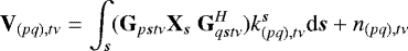
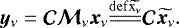
In order to model the complex direction-dependent effects (DDE–station beams, ionosphere, Faraday rotation, etc), we use the Radio Interferometry Measurement Equation (RIME) formalism, which provides a model of a generic interferometer (for extensive discussions of the validity and limitations of the measurement equation see Hamaker et al. 1996; Smirnov 2011). Each of the physical phenomena that transform or convert the electric field before the correlation is modeled by linear transformations (2 × 2 matrices). If ![Mathematical equation: $\vec{s}=[{l},{m},{n}=\sqrt{1-{l}^2-{m}^2}]^T$](/articles/aa/full_html/2018/03/aa31474-17/aa31474-17-eq1.png) is a sky direction, and MH stands for the Hermitian transpose operator of matrix M, then the 2 × 2 correlation matrix V(pq)tν between antennas p and q at time t and frequency ν can be written as:
is a sky direction, and MH stands for the Hermitian transpose operator of matrix M, then the 2 × 2 correlation matrix V(pq)tν between antennas p and q at time t and frequency ν can be written as:
 (1)
(1)
 (2)
(2)
 (3)
(3)
 (4)
(4)
where bpq,t is the baseline vector between antennas p and q. The scalar term  describes the effect of the array geometry and correlator on the observed phase shift of a coherent plane wave between antennas p and q. The 2 × 2 matrix G pstν is the product of direction-dependent Jones matrices corresponding to antenna p (e.g., beam, ionosphere phase screen and Faraday rotation), and X s is referred as the sky term in the direction s, and is the true underlying source coherency matrix. The term n(pq),tν is a randomvariable modeling the system noise. In the following however, we will assume
  and implicitly work on the expected values
  rather than on the random variables (except in Sect. 3.4 and 3.5, where we describe the structure of the noise in the image domain). Making the (tν) indices implicit, we can transform Eq. (2) to:
![Mathematical equation: $\textbf{V}_{pq}=& \displaystyle\sum\limits_{\varphi} \left[ \int_{\vec{s}\in{\mathrm{\Omega}}_{\varphi}} (\JonesMat_p\textbf{X}_{\vec{s}}\ \JonesMat_q^H) k^{\vec{s}}_{pq,\varphi} \right] \\ k^{\vec{s}}_{pq,\varphi}=& \exp{ \left(-2 \mathrm{i}\pi \frac{\nu}{c} \vec{b}_{pq}^T (\vec{s}_{\varphi}-\vec{s}_0)\right)}\\ &\times \exp{ \left(-2 \mathrm{i}\pi \frac{\nu}{c} \vec{b}^T_{pq} \vec{\delta s}_{\varphi}\right)}, $](/articles/aa/full_html/2018/03/aa31474-17/aa31474-17-eq9.png)
where ![Mathematical equation: $\vec{s}_{\varphi}=[\l_{\varphi},\m_{\varphi},\n_{\varphi}]^{T}$](/articles/aa/full_html/2018/03/aa31474-17/aa31474-17-eq10.png) is the direction of the facet phase center and δsφ =s −sφ = [l − lφ, m − mφ, n − nφ] = [δlφ, δmφ, δnφ] are the sky coordinates in the reference frame of facet φ.
is the direction of the facet phase center and δsφ =s −sφ = [l − lφ, m − mφ, n − nφ] = [δlφ, δmφ, δnφ] are the sky coordinates in the reference frame of facet φ.
Applying the term first exponential in Eq. (6) to the visibilities, one still need to apply the position dependent term (second exponential), which can be decomposed as:
 (7)
(7)
The second exponential term is the analog of the w-term corrected for in the W-projection style algorithms. As pointed out by Kogan & Greisen (2009), the first order Taylor expansion approximation of δnφ can be written as:
 (8)
(8)
which, conveniently, can be expressed in terms of a coordinate change in uv:
 (9)
(9)
with  and
and 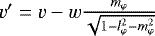 . The linear approximation of δni (Eq. (8)) is plotted in Fig. 1.
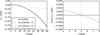 |
Fig. 1 Comparison between the true δni term, and the first-order approximation (right), and residuals (left). The Kogan & Greisen (2009) approximation breaks down away from the facet center (labeled as uv-scaling, dotted line). Applying classical W-projection together with a Kogan & Greisen (2009) style coordinate transformation works better (dashed line), but a blind 3rd–5th-order polynomial works best (solid line). |
2.2 Accurate noncoplanar faceting
As shown in Fig. 1, a more accurate approximation of the  term may be obtained by a fitting a low-order 2D polynomial
 (10)
(10)
where ![Mathematical equation: $\bm{\delta{l}^k_{\varphi}}=\left[1,\delta\l_{\varphi},\delta\l_{\varphi}^2,\hdots,\delta{l}^k_{\varphi}\right]^T$](/articles/aa/full_html/2018/03/aa31474-17/aa31474-17-eq18.png) is a basis function vector for the kth-order 2D polynomial, and Pk,φ is the matrix containing the polynomial coefficients. We can then write
is a basis function vector for the kth-order 2D polynomial, and Pk,φ is the matrix containing the polynomial coefficients. We can then write
![Mathematical equation: ${\vec{b}_{pq}}^T \vec{\delta s}_{\varphi}&= {u}\delta \l_{\varphi}+{v}\delta\m_{\varphi}+{w} (\bm{\delta{l}^k_{\varphi}})^T\bm{\mathrm{P}_{k,\varphi}}(\bm{\delta{m}^k_{\varphi}})\\ &{\overset{\mathrm{def {\overline{\mathrm{P}_{k}}}}}{=\joinrel=\joinrel=}} ({u}+{w} \mathrm{P}_{k,\varphi}^{[10]}) \delta \l_{\varphi}+ ({v}+{w} \mathrm{P}_{k,\varphi}^{[01]}) \delta \m_{\varphi}\\&\ \ \ \ \ \ +{w} (\bm{\delta{l}^k_{\varphi}})^T\overline{\bm{\mathrm{P}_{k,\varphi}}}(\bm{\delta{m}^k_{\varphi}})\\ &{\overset{\mathrm{def {(u',v')}}}{=\joinrel=\joinrel=\joinrel=\joinrel=}} u' \delta \l_{\varphi}+ v' \delta \m_{\varphi} +{w} (\bm{\delta{l}^k_{\varphi}})^T\overline{\bm{\mathrm{P}_{k,\varphi}}}(\bm{\delta{m}^k_{\varphi}})\\ &{\overset{\mathrm{def {{\bm{\mathrm{C}}_{\vec{s}_{\varphi}}}}}}{=\joinrel=\joinrel=\joinrel=\joinrel=}} ({\bm{\mathrm{C}}_{\vec{s}_{\varphi}}}{\vec{b}_{pq}})^T\vec{\delta s}_{\varphi} +{w} (\bm{\delta{l}^k_{\varphi}})^T\overline{\bm{\mathrm{P}_{k,\varphi}}}(\bm{\delta{m}^k_{\varphi}})$](/articles/aa/full_html/2018/03/aa31474-17/aa31474-17-eq19.png)
where  is equal to P k,φ with the coefficients
 ![Mathematical equation: $\mathrm{P}_{k}^{[01]}$](/articles/aa/full_html/2018/03/aa31474-17/aa31474-17-eq21.png) and
and ![Mathematical equation: $\mathrm{P}_{k}^{[10]}$](/articles/aa/full_html/2018/03/aa31474-17/aa31474-17-eq22.png) in cells [0, 1] and [1, 0] zeroed. Based on this polynomial fit, we compute a series of convolutional kernels which we term fw-kernels (for “fitted w kernels”), and apply them by exact analogy with W-projection. As in Kogan & Greisen (2009), we can see here that the first order coefficient of the polynomial fit P k,φ is equivalent to a w-dependent (u, v) coordinate scaling. This has the effect of taking off the main component of the w-related phase gradient, and thereby reducing the fw-kernels’ support size (step from Eq. (11) to Eq. (12)) that depends on (i) the w-coordinate, (ii) the facet diameter and (iii) its location. In practice, if the facets are small enough (as it is the case when applying DDEs–see Sec. 3), the support of the fw-kernels is only marginally larger than the spheroidal-only kernel. The fw-kernels are computed per facet, per a given w-plane, as
in cells [0, 1] and [1, 0] zeroed. Based on this polynomial fit, we compute a series of convolutional kernels which we term fw-kernels (for “fitted w kernels”), and apply them by exact analogy with W-projection. As in Kogan & Greisen (2009), we can see here that the first order coefficient of the polynomial fit P k,φ is equivalent to a w-dependent (u, v) coordinate scaling. This has the effect of taking off the main component of the w-related phase gradient, and thereby reducing the fw-kernels’ support size (step from Eq. (11) to Eq. (12)) that depends on (i) the w-coordinate, (ii) the facet diameter and (iii) its location. In practice, if the facets are small enough (as it is the case when applying DDEs–see Sec. 3), the support of the fw-kernels is only marginally larger than the spheroidal-only kernel. The fw-kernels are computed per facet, per a given w-plane, as
 (15)
(15)
In practice, a 3rd to 5th-order polynomial is sufficient to accurately represent the w-related phase variation across a given facet.
3 Imaging in the presence of direction dependent effects
In this section, we describe, in terms of linear algebra, how the DDEs are taken into account in the forward (gridding) and backward (gridding) imaging steps.
Specifically, we describe how the dirty images and associated PSFs are constructed from the set of direction-time-frequency dependent Jones matrices. We show in Sect. 3.1 that, in general, in the presence of baseline-time-frequency dependent effects, the linear mapping  (Eq. (18) below) between the sky and the dirty image is not a convolution operator. However, in Sect. 3.5, we describe a first-order image correction that modifies this function into a direction-dependent convolution operator, under the condition that the Mueller matrices are approximately baseline-time-frequency independent. As shown in Sect. 3.6, this correction is not sufficient, and the effective PSF retains a directional variation. “Local” PSFs then have to be estimated per facet. In this way, the normalized linear mapping
  (Eq. (30) below) can be understood as a local convolution operator.
3.1 Forward and backward mappings
In order to study the properties of the linear function, it is convenient to describe this mapping from image to visibility space and back performed by the algorithm using linear algebra. For a given sample of 4 visibility products, Eq. (1) can be written in terms of a series of linear transformations:
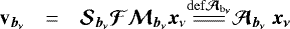 (16)
(16)
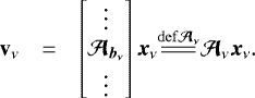
where  is the visibility 4-vector sampled by baseline b = (p, q, t) at frequency ν (for most of this section, we assume a narrow-band scenario). If nx is the number of pixels in the sky model, the true sky image vector xν has a size of 4nx , and for each sky pixel i = 1…nx, the four corresponding correlations3
  or
or  are packed into xν starting from index 4i. Then,
  represents the DDEs, and is a (4nx) × (4nx) block diagonal matrix. For any given image pixel i, the corresponding 4 × 4 block of
  is the Mueller-like4 matrix associated with the pixel direction si:
  .
.  is the Fourier transform operator of size (4nv) × (4nx). Each of its (4 × 4) blocks is a scalar matrix, the scalar being the kernel of the Fourier basis
  (see Eq. (2)). The matrix
  is the sampling matrix, size 4 × (4nv), which selects the 4 visibilities corresponding to bν
For the full set of nv 4-visibilities associated with channel ν, which we designate as Ων, (bν ∈ Ων then means that the bν index can be taken to represent a visibility index from 1 to nv), we can stack nv instances of Eq. (16) to write the forward (image-to-visibility) mapping as:
 (17)
(17)
Note that  represents the “ideal” mapping from images to visibilities, in the sense that a unique DDE is applied at every pixel (ignoring the approximation inherent to pixelizing the sky, we can say that
  represents the true instrumental response). Implementing
  directly in the forward (modeling) step of an imager would be computationally prohibitive: it is essentially a DFT (Direct Fourier Transform) with pixel-by-pixel application of DDEs. Existing approaches therefore construct some FFT-based (Fast Fourier Transform) approximation to
  . The convolutional function approach, i.e. AW-projection, approximates
  by a single FFT followed by convolutions in the uv-plane during degridding. The facet-based approach of the present work segments the sky xν into facets, then does an FFT per-facet, while applying a constant DDE
  (where s φ is the direction of facet φ). The resulting approximate forward operator,
  , becomes exactly equal to
  in the limit of single-pixel facets (see Sect. 3.7 for a further discussion).
3.2 Forming the dirty image
Since  is generally noninvertible, imaging algorithms tend to construct the adjoint operator
  , or some approximation thereof
  , to go back from the visibility domain to the image domain5. This amounts to forming the so-called dirty image.
In the framework of facets and DDE calibration, we obtain what is at best an estimate  (due to finite facet sizes, and also calibration errors), and therefore the adjoint operator being applied is also an approximation. The same applies to convolutional gridding approaches. For the purposes of this section, however, letus assume that the approximation is perfect. We then have the following for the dirty image vector yν :

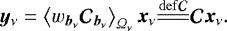
where  is a diagonal matrix containing the set of weights
  at frequencyν. Note that the weighted sum comes about due to the block-column of Eq. (17) being left-multiplied by its conjugate, a block-row.
For each bν, the matrix 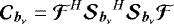 is a convolution, as a direct consequence of the Fourier convolution theorem. This matrix represents the convolution of the sky by the PSF corresponding to a single uv-point (i.e. a single fringe). In the absence of DDEs (
 ), the linear mapping
  can be written as a a weighted sum of such matrices, and is therefore also a convolution:
 (22)
(22)
This is just the familiar result that in the absence of DDEs, the dirty image is a convolution of the apparent sky by a PSF.
Below, we show that in the presence of DDEs (even corrected-for DDEs), this relationship generally ceases to be a true convolution. We will also show that, under certain conditions, the mapping can be modified (at least approximately) into a local convolution, i.e. one where the PSF varies only slowly with direction. This distinction is important: most minor-loop deconvolution algorithms such as CLEAN either assume the problem is a true (global) convolution, or can be trivially modified (at least in the faceted approach) to deal with a local convolution problem, i.e. a position-dependent (per facet) PSF.
3.3 Toeplitz matrices and convolution
Any matrix C representinga one-dimensional convolution is Toeplitz, and vice versa. A Toeplitz matrix is a matrix in which each descending diagonal is constant, i.e. Cij = Ci+1,j+1 ≡ ci−j. We now show that a similar property, which we’ll call Toeplitzian, can be defined for convolution of 2D, 4-polarization images. We can then discuss how DDEs break the convolution relationship by making the matrix representing the tranfer function less Toeplitzian.
First, consider matrices that represent 2D convolution of scalar (unpolarized) images. The pixel ordering, i.e. the order in which we stack the pixels of a 2D image into the image vectors x and y, induces a mapping from vector index i to pixel coordinates (li , mi). Given a fixed pixel ordering, consider a matrix C whose its elements are constant with respect to a translation of pixel coordinates, i.e.  for all ij and i′ j′ such that
  and
and  . There then exists a function of pixel coodinates c(l, m) such that for all ij
 (23)
(23)
and it is then easy to see that applying the C matrix to the image vector x corresponds to a 2D convolution of the corresponding image by c, and vice versa. For an n × n image, assuming the conventional pixel ordering of stacked columns (or rows), the matrix C is composed of n × n blocks, each block being an n × n Toeplitz matrix. Each constant descending diagonal in each such block represents a constant pixel separation Δl, Δm. In other words, Cij is constant for any pair of pixels having the same pixel separation Δl, Δm.
To generalize this to 4-polarization images, we simply replace Cij in Eq. (23) by a 4 × 4 scalar matrix. Our general Toeplitzian matrix is then composed of n × n blocks, each block being a 4n × 4n Toeplitz matrix composed of 4 × 4 scalar matrices. Each column of such matrix represents the convolution kernel (or PSF), shifted to the position of the appropriate image pixel.
The linear function defined by the PSF  or
or  is Toeplitzian, with 1 on the main diagonal (corresponding to the peak of the PSF). We focus on two regimes in which a matrix becomes non-Toeplitzian. The first one is simple, when Cij in Eq. (23) is constant to within a 4 × 4 per-column scaling factor Mj. This correponds to an attenuation of the image by
  , followed by a convolution:
 (24)
(24)
This regime arises when trivial (i.e. non time-baseline dependent) DDEs are present and not accounted for when forming the dirty image.  can be factored out of the sum in Eq. (21) and absorbed into the apparent sky
  . In this case we can still talk of the PSF shape being constant across the image.
The more complex regime arises when the mapping is non-Toeplitizian in the sense that the shape of the PSF changes across the image. This naturally arises when nontrival DDEs are present and not accounted for, and the dirty image is the weighted sum of the sky affected by baseline-dependent DDE
 (25)
(25)
More subtly, even if DDEs are perfectly known and accounted for in  , the resulting function is, generally, not a convolution, in the sense that the shape of the PSF becomes direction-depedent. This is obvious in the case of nonunitary
  (since its amplitude essentially appears twice in Eq. (21), and the resulting dirty image requires renormalization – we will return to this again below). Less obvious is that this holds, generally, even for unitary
  . Consider the simple case of a scalar, unitary DDE (i.e. a phase term affecting both polarizations equally). This corresponds to a diagonal
  with Mi = eıψi on the diagonal. If the matrix elements of
  are given by Cij, then each element of
  , i.e. the response at dirty image pixel j to a source at pixel i (i.e. the PSF sidelobe response), is given by
 (26)
(26)
It is easy to see that the (Toeplitzian) condition of Eq. (23) is only satisfied if ψj − ψi is constant for any pair of pixels having the same pixel separation Δl, Δm. This condition is only true for a linear phase slope over the image.
We have shown that here all nontrivial DDEs, including unitary ones, with the exception of linear phase slopes, generally result in a direction-dependent PSF even when perfectly known and accounted for via Eq. (18). Note that this equation (or some approximation thereof) is applied by all existing imagers. If we consider the w-term as a DDE (see, e.g., Smirnov 2011), we can see that W-projection and W-stacking also represent approximations of Eq. (18), and therefore still yield a direction-dependent PSF.
3.4 Loss of local convolution property and nonuniform noise reponse
Equations (23) and (26) give us a framework in which we can reason about the degree of direction-dependence in the PSF. The pixel separation Δl, Δm corresponds to the PSF sidelobe at Cij . Thus, the direction-dependence of a particular PSF sidelobe Δl, Δm is determined by the variation of the Mueller matrix across the image on a length scale of Δl, Δm. For direction-dependent effects that are locally approximately linear (i.e. close to the form of Eq. (26)), the problem is locally a convolution. As long as this is true, and assuming  is known, one could in principle incorporate knowledge of a local direction-dependent PSF into the minor cycle deconvolution algorithm, using the linear function defined above to form up the dirty images. In the context of facet imaging this seems straightfoward, as we can simply compute a PSF per facet (see below). However, if the Mueller matrices are nonunitary,
  has two very undesirable properties.
Firstly, as is clear from Eq. (26), the PSF sidelobe response  is coupled to
  at both positions i and j. Ideally, we would like to decouple the PSF sidelobe response from the DDE at position i.
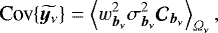
Secondly, consider the thermal noise response in the dirty image given by  . Thermal noise can be assumed to be independent and identically distributed Gaussian in the visibilities
  . If a is a vector of random variables and b = Ba, then the covariance matrices of the two vectors are related by Cov{b} = BCov{a}BH. Applying this to Eq. (18), and using
  for the variance of the real and imaginary parts of each visibility, we get
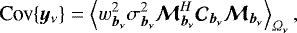 (27) spatially uniform. In particular, the variance (of the four polarization products) at each pixel i is given by
 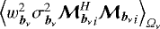 .
.
3.5 Image-plane corrections
We show in this section that when  is approximately baseline-time independent (at a given frequency), we can find a dirty image correction that brings
  back to a direction-dependent convolution operator. This is a reasonable assumption in general if the fractional bandwith of the data chunk is small enough6, and in this case we can write
![Mathematical equation: $\bm{\mathcal{T}}{\mathrel{\overset{\mathrm{def {{\widetilde{{{\bm{\mathcal{M}}_{\nu}}}}}}}}{\scalebox{3}[1]{\begin{inlinestripns}{si241}$\approx$](/articles/aa/full_html/2018/03/aa31474-17/aa31474-17-eq85.png)
We can see from Eq. (28) that we can construct a modified normalized image
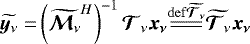 (30)
(30)
mapping. The columns i of  are then the PSF of a source centered on pixel i, and they only differ one to the other by a matrix product. In other words, the PSF centered on pixel i is the same as the PSF centered on pixel j to within a constant. Strictly speaking
  is not a convolution matrix, but we will refer to it as a direction-dependent convolution matrix. An alternative way to look at this is to write
  where
where  is the apparent beam-attenuated sky.
In order to obtain  , we can see from Eq. (28) that although
  is not block diagonal, each ith (4 × 4) block on its diagonal is
![Mathematical equation: $ {{\bm{\mathcal{T}}_{\nu}}}[i,i]=\left<w_b {{\scriptstyle \bm{\mathcal{M}}}}^H_{b,i}{{\scriptstyle \bm{\mathcal{M}}}}_{b,i}\right>_{{\Omega_{\nu}}}. $](/articles/aa/full_html/2018/03/aa31474-17/aa31474-17-eq93.png) (31)
(31)
Assuming approximate baseline-time independence at ν of the direction-dependent local convolution function (i.e. ![Mathematical equation: ${{\bm{\mathcal{T}}_{\nu}}}[i,i]\approx\widetilde{{{\scriptstyle \bm{\mathcal{M}}}}_i}^H\widetilde{{{\scriptstyle \bm{\mathcal{M}}}}_i}$](/articles/aa/full_html/2018/03/aa31474-17/aa31474-17-eq94.png) ), we get
), we get
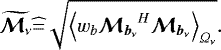 (32)
(32)
If the assumption in Eq. (28) holds (definition of  ), then the image plane correction exists, and it is given by Eq. (32). Furthermore we take into account the deviation from this approximation by using the local PSF (Sect. 3.6) in our deconvolution algorithms (Sect. 4). Applying the
  correction in Eq. (27), the normalized image-plane pixel covariance
  becomes
 (33)
(33)
and  is spatially uniform.
In practice, the Mueller blocks in  are assumed to be diagonally dominant and are reduced to scalar matrices when computing
  .
.
3.6 Direction-dependent PSFs
As shown above, the combined effects of (i) baseline-time-frequency dependence of the DDEs, and (ii) decorrelation cause the linear mappings  and
and  not to be exact convolution matrices. Specifically, the large fractional bandwidth makes the beam pattern vary significantly toward the edge of the field, and the effective PSF is also direction-dependent. All modern imagers are indeed affected by problem (i) in the minor cycle, and problem (ii) in both the major and minor cycles, and so will produce morphologically biased results away from the pointing center. In this section we describe how ddfacet takes into account and compensates for these effects.
3.6.1 Effect of decorrelation
It follows from Eq. (1) that any source in the sky corresponds to a complex vector rotating in the uv-domain and any visibility measurement is an averaged value over that domain. This fact causes the amplitude of the averaged vector to decrease (in the extreme case in which the phase of the complex vector ranges over [−π, π] in the domain of averaging, the average vector amplitude can be zero). This effect is known as decorrelation and is described in much detail by Bridle & Schwab (1999), Thompson et al. (2001), Smirnov (2011), Atemkeng et al. (in prep., and references therein). One can see from Eq. (1) that the magnitude of decorrelation depends on (i) the baseline coordinates and (ii) the distance of the source to the phase center, causing the effective PSF to be direction-dependent. This effect is a direct image-domain consequence of baseline and direction-dependent decorrelation, and is known in the literature as smearing.
The effective mapping is therefore direction-dependent, and no imaging and deconvolution can take this effect into account. This has the direct effect of incorrectly estimating the source’s morphology, and the error gets worse as the source gets further away from the phase center. Since the longest baselines are most affected, decorrelation is minimized by accepting a small decorrelation (e.g. a few per cent decrease in the ratio to peak to integrated flux density) at the edge of the field.
A major strength of a facet-based imaging and deconvolution framework is that we can take decorrelation into account in quite an easy way by computing a PSF per facet. While computing the PSF, each unit visibility is multiplied by the factor γpq,t, defined as
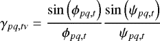 (34)
(34)
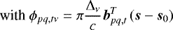 (35)
(35)
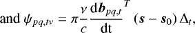 (36)
(36)
where Δt and Δν are the time and frequency size for the domain over which the given visibility has been averaged, and  is the speed of the baseline in the uv domain. Conversely, in the forward step of major cycle, γpq,tν can be applied to the model visibilities on a per-facet basis. This allows decorrelation to be properly accounted for both in the minor and major cycles.
3.6.2 Per-facet PSFs
In the facet approach, it is staightforward to compute a per-facet PSF that takes all of the above effects into account during deconvolution. We compute a PSF per facet ϕ for a point source following
 (37)
(37)
where  is the local convolution function function in facet ϕ, and 01 is a vector containing zeros everywhere except the central pixel, which is set to the value {I, Q, U, V } = {1, 0, 0, 0} Jy. Figure 3 shows the PSF evaluated for a source in two different facets.
Note that in the full-polarization case, i.e. given DDEs with a nontrivial polarization response (nondiagonal, or at least nonscalar Mueller matrices), it is in principle incorrect to speak of one PSF. All four Stokes components are, in general, convolved with different PSFs, and there are also “leakage PSFs” that transfer power between components. A fully accurate description of the local convolution relationship therefore requires that 16 independent PSFs be computed, with all the consequent expense (i.e. 16 separate gridding operations for the PSF computation). In practice, we limit ourselves to computing the Stokes I PSF, and, during the minor cycle of deconvolutin, assume that the other Stokes component PSFs are the same, and treat leakages as negligible, trusting in the major cycle to correct the effect. The impact of this approximation on polarization deconvolution is a topic for future study.
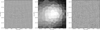 |
Fig. 2 The nonunitary Mueller matrices in |


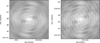 |
Fig. 3 PSF estimated at various locations of the image plane even after the transformation described in Eq. (30) is applied. The net local convolution function significantly varies, and this effect is taken into account by computing a PSF per facet. |
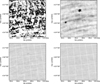 |
Fig. 4 Residual data for a fraction of the field of view of the simulation described in Sect. 6. The left to right and top to bottom panels show the iterations {0, 1, 2, 3}. As explained in Sect. 4.2.1, the ssd algorithm works differently from a matching pursuit in that it does joint deconvolution on subsets of pixels, and the estimated flux is fully removed at each iteration. The ssd has remarkable convergence properties. |
3.7 In-facet errors
As explained in Sect. 1, the facet-based imaging and deconvolution framework presented here has the disadvantage of taking DDEs into account in a discontinuous manner in the image domain. Indeed, within a direction-dependent facet, DDEs are assumed to be constant while they continuously vary. This is typically the case for beam effects that vary very quickly, especially around the half power point. We show in this section that this effect can be partially accounted for by applying a spatially smooth term to the image  .
.
In this section we estimate the flux density error across a given facet φ that arises due to the fact that the Jones matrix has been assumed to be spatially constant. Following Eq. (16), the residual visibility on a given baseline b can be written as
 (38)
(38)
where  is a (4nx) × (4nx) block diagonal matrix which represents the direction-independent Jones matrix that has been assumed for that facet, and
  is the sky that has been estimated. We assume the deconvolution algorithm is subject to an
  -norm constraint, and
 (39)
(39)
is minimized, giving
 (40)
(40)
and therefore
 (41)
(41)
As in Sect. 3.5, assuming the  and
and  are baseline-time independent at ν we get
 (42)
(42)
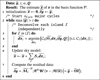
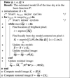 |
Algorithm 1 hmp deconvolution algorithm. Here t is a user defined flux density threshold, α is a minor cycle loop gain. Other symbols are defined in Table 1 and/or in the main text. |
One can see that when no DDEs are being applied during deconvolution ( , as is traditionally done in radio astronomy), one can correct the fluxes by applying a smooth beam correction in the image domain.
4 Wideband deconvolution
In this section, we describe how we solve for the sky in the local deconvolution problem as well as the global inverse problem7  . We present two multiscale wideband deconvolution algorithms that iteratively estimate the underlying true sky. In contrast to the calibration problem, the deconvolution problem is linear, but is strongly ill-conditioned. A wide variety of algorithms have been developed to tackle the conditioning issue.
The first and largest family of deconvolution algorithms in radio interferometry is based on compressive sampling theory (or compressive sensing), and assumes the sky can be fully described by a small number of coefficients in a given dictionary8 of functions (a sparse representation). The dictionary of functions can be, but is not necessarily, a basis function from deltas to shapelets. In practice and for a given dataset, a specific convex solver is used to estimate the coeffiscient associated to the functions of the dictionary. The cost function is often an  -norm subject to an
  constraint. The widely used clean algorithm is one of those9 solvers, but we can also mention moresane (Dabbech et al. 2015), or sasir (Garsden et al. 2015). Each one of these methods uses a specific solver to estimate the coefficients associated with a given dictionary. The second family of algorithms deals with ill-conditioning using Bayesian inference.
Only a few existing algorithms are able to accurately estimate flux densities as well as intrinsic spectral properties (while taking Jones matrices into account). The most efficient and widely used of these is the mtms-clean algorithm (for multi-term multi-scale, see Rau & Cornwell 2011, and references therein). Bhatnagar et al. (2013) have extended this algorithm in order to take time-frequency dependent DDEs into account. The drawbacks of this algorithm combination are that (i) since each Taylor coefficient image stacks information from potentially large fractional bandwidth,  (Eq. (30), Sect. 3) will tend not to be a convolution operator, (ii) it decomposes the signal in terms of Taylor basis functions, and the signal needs to be gridded nt -times if nt is the number of Taylor terms, and (iii) baseline-dependent averaging cannot be used with A-Projection (see Sect. 5.2).
Instead, we produce a (nch × npix) spectral cube, the dirty images of size (npix) being formed into the corresponding nch frequency chunks. The spectral cube then contains information about the sky’s spectral properties. We present in this section two wideband deconvolution algorithms that estimate flux densities as well as the intrinsic spectral properties (taking into account Jones matrices such as primary beam direction-time-frequency behavior). The first uses a variation of the matching pursuit clean algorithm, while the second uses a genetic algorithm.
4.1 hmp deconvolution
In this section we present the hmp deconvolution algorithm (Hybrid Matching Pursuit). The idea is quite simple and consists of decomposing the signal around the brightest pixel i in the spectral cube  into a sum of components with different spatial and spectral properties. The basis function is similar to mtms-clean (Rau & Cornwell 2011), but the idea differs in that (i) we grid the data only once (we do not create dirty images at different resolutions and for different Taylor terms), (ii) the optimisation step is done on a set of pixels (and not only on the brightest pixel), and (iii) at each iteration all coefficients are estimated in the chosen basis function (as opposed to the maximum coefficient only). This last point is illustrated by the example of a faint extended signal containing a brighter point source. While Cornwell (2008) have to introduce an ad hoc “small-scale bias” to reconstruct the compact emission, we aim at finding nonzero coefficients for the point source and the extended emission, at each iteration (the same applies to the spectral axis). The following algorithm is implemented in ddfacet, natively taking direction-dependent residual images and associated PSFs into account (see Sect. 3.5 for a discussion of the normalization).
We first choose a set  of functions into which we want to decompose the spectral cube. For example, it can be made of Gaussians with various sizes and spectral indices. The sky image
  of models centered on pixel i at a frequency ν is then written as

where  is the (nx × np) matrix containing the spectro-spatial dictionary estimated at frequency ν, and πi is the spectro-spatial sky model of pixel i, containing the np parameter values of the spectro-spatial dictionary. We can then write the contribution
  of pixel i to the spectral cube as

where ν is the frequency chunk and  is the normalized spectral PSF. In short,
  maps the vector of spatio-spectral coefiscients π for all pixels to the spectral cube
  , taking into account the local spectral PSFs.
The algorithm is described in detail in Alg. 4. Particular attention needs to be given to step 5 where we estimate the best local model by minimizing a cost function. Different cost functions give different variations of hmp. Relaxing the constraint  , we can for instance set
  as
as
 (49)
(49)
Overview of the mathematical notations used throughout this paper.
where the  norm
norm  of x is computed for the metric Q, with Q being in practice a tapering function. The least-squares solution is then given by the pseudo-inverse
![Mathematical equation: $ \widehat{{\vec{\pi}_{i}}}&=\left[{{\widetilde{\mathrm{\bm{\Theta}}_{i}}}}^T\bm{Q}\ {{\widetilde{\mathrm{\bm{\Theta}}_{i}}}}\right]^{-1}{{\widetilde{\mathrm{\bm{\Theta}}_{i}}}}^T\bm{Q}\ {\widetilde{\vec{y}}}. $](/articles/aa/full_html/2018/03/aa31474-17/aa31474-17-eq142.png) (50)
(50)
Alternatively, we can use a Non-Negative Least Squares (NNLS) optimisation in step 5 (Alg. 4) by setting  as in Eq. (49) while constraining the solution using
  . In our experience the hmp-nnls gives the best results in reconstructing extended emission.
4.2 Wide-band joint subspace deconvolution
In this section, we describe the ssd (SubSpace Deconvolution algorithm). It is a generic hybrid joint deconvolution algorithm that uses subspace optimisation. We present in Sect. 4.2.1 the generic scheme for subspace optimisation in the framework of deconvolution, and in Sect. 4.2.2 we present one such algorithm that uses a genetic algorithm in the optimisation step (ssdga).
4.2.1 Subspace optimisation for deconvolution
It is well known that deconvolution algorithms based on Matching-Pursuit solvers (specifically clean) are not robust in the deconvolution of extended emission. Joint deconvolution algorithms are more robust, as demonstrated by Garsden et al. (2015), but are not useful with large images since their sizes can exceed  pixels. Indeed, Eq. (48) is costlyto invert because
  is expensive to apply10 the data. Therefore in order to make joint deconvolution practical with real life data-sets, we aim at incorporating it in a matching pursuit-type scheme. As for hmp (Sect. 4.1), the idea is to decompose the signal into a basis function but here the parameter space at each iteration is not a set of coefficients for one pixel only, but for a subset
  of pixels in thespectral cube (an island).
To illustrate the idea of ssd, consider the global transfer function in Eq. (48). Since the convolution matrix is diagonally dominant (the PSF goes to zero far from the center), the main idea is that distant regions can be deconvolved separately. This amounts to building an operator  with zeros where
  is considered to be negligible such that
  , and the deconvolution is done jointly within each subspace
  of the global {π} parameter space. This approximation will however lead to biases in the estimate
  of π, because the contribution of the sky in island
  to the observed flux in island
  has been neglected.
This will happen for example when a bright (a) source in an  island has a faint (b) source (
 island) in its side-lobe, and when the two islands are deconvolved independently. The faint source flux can be over- (or under-) estimated in the first iteration since the cross-contamination term is ignored. However if one computes the global residual map in a second iteration, most of the side-lobe of source (a) has been properly removed at
  . If the islands are jointly deconvolved again, the sky model estimate will be better than in the previous iteration. In our experience, this algorithm has remarkable convergence properties.
The ssd algorithm is described in detail in Alg. 4. Given a residual image, in a first step the brightest regions are isolated and joint deconvolution is performed independently on groups of pixels (here called islands) using the local convolution operator  with
with  , where
  is an
is an  matrix that maps the
  pixels of island
  onto the full set of npix pixels. For example we can minimize the cost function by setting
 (51)
(51)
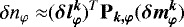
where  are the differential values of the spatio-spectral coefficients in a given basic function (see Sect. 4.1).
In a second step, the union of the sky models are subtracted from the visibilities, and the visibilities are re-imaged (corresponding to the step  ).
).
The conditions for the convergence of ssd are hard to find, but depend on the structure of  compared to
  . We can estimate at step k the contribution to the observedflux
  in
in  of all islands
  . If
. If  is the error in the estimate
 of x, we can write
 (52)
(52)
Since each island  is deconvolved in its own subspace (independently of other islands), the level of the flux density bias at iteration k + 1 is

Assuming the structures of the side-lobes of the different  in
in  are uncorrelated, the power in the cross-island terms averages out in the quadratic sum, and we get

 |
Algorithm 2 ssd deconvolution algorithm. Here t is a user defined flux density threshold. |
Here  is the power in the side-lobes of all islands
  to islands
  . If the cross-contamination power is small enough ssd converges. For example, in the trivial case of two single pixel islands with equal flux s, and cross-contamination term p (the PSF of
  onto
onto  and conversely), at iteration k we have

and ssd always converges.
4.2.2 An example of ssd using genetic algorithm
We have presented in Sect. 4.2.1 the ssd algorithm, which carries out joint deconvolution over a set of sub-spaces in an independent manner. In this section we detail how the genetic algorithm in ssdga implements step 4 in Alg. 4. Specifically, we discuss an example of an ssd algorithm, where we perform step 4 (Alg. 4) using a genetic algorithm (ssdga). Genetic algorithms are very different from convex solvers in the sense that they are (i) combinatorial and (ii) nondeterministic. While genetic algorithms are rather simple to use and very flexible, ssdga is in principle good for the deconvolution of extended signal. We can for instance optimize the  norm which is a nonconvex problem.
This step corresponds to fitting the residual dirty image by a spectral sky-model for each island  , convolved by the local spectral PSF.
Our current implementation is based on the deap package (Fortin et al. 2012). Each individual ‘sourcekin’ consists of aset of fluxes together with a spectral index. Each sourcekin is a spectro-spatial model of the sky in  . It could also include minor axis, major axis, and position angle of a Gaussian for example. The idea consists of building and evolving the population of sourcekin, and the fitness function is set to be
  in our case. An example of spectral deconvolution using ssdga is presented in Sect. 6.
5 Implementation, performance and features
The bulk of ddfacet is implemented in Python 2.7, with a small performance-critical core module (gridding and degridding) written in C. In this section we discuss some important aspects of the implementation. In Sect. 5.1, we describe aspects of parallelization. In Sect. 5.2, we describe how we use a baseline-dependent averaging scheme in the context of wide-field wideband spectral deconvolution, and we explain how we handle the nonregular spatial domains of Jones matrices in Sect. 5.4. In Sect. 6 we demonstrate our imaging and deconvolution framework on a single simulation.
5.1 Parallelization
The gridding, degridding and FFT operations of faceted imaging are embarrassingly parallel, as every facet can be processed completely independently. The ddfacet implementation is parallelized at the single-node level, using the Python multiprocessing package for process-level parallelism, and a custom-developed process manager called AsyncProcessPool that implements asynchronous, on-demand, multiprocessing akin to the concurrent futures11 module found in Python 3. The bulk of the data (visibilities, uv-grids and and images) is stored in shared memory using the SharedArray12 module, and a custom extension called shared_dict. This significantly reduces the overhead of inter-process communication. This also allows us to perform I/O and computation concurrently: a successive data chunk is read in while gridding of the previous chunk proceeds. In the minor cycle, we employ the same technique to parallelize the ssd algorithm. For hmp deconvolution (and other CLEAN-style minor loops), the minor loop is inherently serial, but a reasonable speedup is achieved with minimum effort by employing the numexpr package13 to vectorize large array operations.
All this allows ddfacet to make very good use of multiple cores in a NUMA architecture, maintaining high core occupancy throughout any given imaging run. We are conducting detailed performance studies and these will be the subject of a separate paper. Here we present the summary results of a simple parallelisation scaling experiment.
We perform an imaging run using 14 h of VLA (C+D configuration) data for the field around the source 3C147, in L-band. This totals 2 350 127 time-baseline samples, with 64 channels each, for a total bandwidth of 256 MHz. We make 5100 × 5100 pixel images of a 2.8° × 2.8° field tiled by 23 × 23 = 529 square facets, in two frequency bands of 128 MHz each. A (rotating) primary beam model is applied on a per-facet basis. We run 5 major cycles of hmp CLEAN, down to an absolute flux threshold of 0.4 mJy.
Our test machine has two Intel Xeon E5, Sandy Bridge class CPUs, each with 8 physical cores and 16 virtual cores (hyperthreading enabled). In serial mode, i.e. with all operations running on a single core, we measure a total “wall time” for this imaging run of about 12 h. Ninety four% of this time is spent in the gridding. We then increase the number of parallel processes, and plot the resulting speedup factor (in terms of wall time, thus including all overheads) in Fig. 5. We see exemplary linear scaling of performance up to 16 processes (i.e. to the point where each physical core is occupied by a single process). Beyond this point, the scaling relation declines, as processes running on virtual cores start competing for resources of a single physical core. Note that a speedup factor of 12 from 16 cores is excellent efficiency: a quick calculation shows that this corresponds to 98% of the computation being parallelized.
From this we can conclude that our parallel implementation scales linearly with available physical cores, while the benefits of hyperthreading are marginal in comparison. We also find that the computational cost of the gridding step dominates overall processing. ddfacet therefore implements two strategies for reducing the overall cost of gridding: baseline-dependent averaging (BDA) and sparsification.
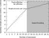 |
Fig. 5 Speedup factor (in terms of overall wall time) obtained by running ddfacet on multiple cores. The solid line corresponds to fixed affinities (each worker process was pinned to a single CPU core), while the dashed line to no affinities (the OS scheduler was allowed to migrate processes across cores). In the former case, processes 0–7 were pinned to the first physical CPU, and 8–15 to the second CPU. This explains the slightly better performance in the no-affinities regime with ≤8 processes, as the OS scheduler was allowed to make use of the second CPU. The graph also shows significanly worse scaling in the hyperthreaded regime. |
5.2 Baseline-dependent averaging
Averaging visibilities has the effect of reducing data volumes and increasing computing efficiency. However, information is unavoidablylost in the process, and therefore inverting the Measurement Equation from the averaged (and therefore smaller) set of visibility measurements is, numerically, subject to poorer conditioning.
The metric we use to limit the loss of information is based on decorrelation effects14 , and those will indeed constrain the maximum time and frequency domain over which visibilities can be averaged. It can be seen from the rime (Eq. (1)) that decorrelation can be caused by the variation over time, frequency and direction of (i) the Jones matrices or (ii) the sky, and most importantly (iii) the geometric phase term (the kernel k term in Eq. (1). Decorrelation due (i) and (ii) largely depends on the target, the instrument and the observing frequency. For example, low-frequency ν ≲ 300 MHz data (such as that taken by the LOFAR telescope) is affected by ionospheric phase, which varies on the timescale of 10–30 s (and is also direction-dependent due to the large FoVs). At higher frequencies, tropospheric phase begins to have a similar (although effectively direction-independent) effect. The decorrelation due to (iii) is well understood and predictable. For a given direction s, if the phase varies linearly across the time or frequency domain  , and one canwrite

where  and
and  are the baseline vectors (in units of wavelength) at the edges of the domain
  .
.
Interferometric data is typically conservatively averaged at best, using a common time-frequency bin across all baselines that corresponds to no more than a few percent amplitude loss on the longest baseline for a source on the edge of the field of view. Several authors have come to the conclusion that this is sub-optimal, and that one could use BDA instead (see Cotton 1989, 1999; Atemkeng et al., in prep.), with more aggressive averaging on the shorter baselines, since for a given direction, time and frequency domain, they decorrelate less than the longer baselines. With core-heavy arrays such as MeerKAT and SKA1, the potential storage savings of BDA can be substantial, since the data sets are dominated by short spacings.
It is important to keep in mind that, for purposes of data storage, the largest time/frequency domain to which any given baseline may be averaged is given by
 (62)
(62)
where  ,
,  , and
, and  are the domains corresponding to an acceptable decorrelation for (i) the Jones matrices, (ii) the sky, and (iii) the geometric phase term respectively. In the presence of DDEs such as the ionosphere,
  is the term that typically constrains
  , because there is no way to correct the stored visibilities for the DDEs; rather, we need to apply Jones matrices to the data during imaging, as described in Sect. 3 (see Eqs. (17) and (18)). For example, consider a single baseline at low frequency, having a decorrelation time scale of the geometric phase term of the order of a few minutes. As the Jones matrices corresponding to the ionosphere are direction dependent, and vary on an approximately ten second time scale, one cannot average the stored data on time scales larger than seconds without substantially degrading the imaging response.
Even if the storage economies of BDA are not realized (and are in any case limited by  ), ddfacet derives computational economies from this technique. If one assumes that the sky term is constant across
  , one can average the 2 × 2 visibilities over
  , while applying the per-facet phase rotations, and the (direction-dependent) Jones matrices, to each individual visibility. This is done on-the-fly in the gridder and degridder code. The actual gridding (or degridding) is then done once per averaging domain, rather than once per visibility. The resulting savings can be substantial, since averaging visibilities involves fewer FLOPS than applying the convolution kernel inherent to gridding or degridding. The BDA gridding algorithm implemented in ddfacet is presented in detail in Alg. 8. We note that a similar approach has been implemented in recent versions of WSCLEAN (Offringa et al. 2014), without the direction-dependent Jones correction.
On-the-fly BDA in the context of faceting offers an interesting performance trade-off. Note that  is determined by facet size, rather than the full FoV size. While imaging smaller facets, more agressive BDA may be applied, since more visibilities can be averaged before a given decorrelation level is reached. Note that at the limit of single-pixel facets, per-facet BDA reduces to averaging the entire (phase-shifted) dataset, which is effectively the same as doing a DFT. Figure 6 shows thecompression ratio achieved for a few fixed decorrelation levels, as a function of number of facets (across the same FoV), for a VLA B-configuration obervation. Note that more core-heavy configurations such as MeerKAT and SKA1-MID should be able to achieve even higher compression ratios. Figure 7 shows the resulting speedup in gridding time per facet. Note that the speedup flattens out at around a factor of 4. Presumably, at this point the gridder performance becomes dominated by memory access. Thus, the computational cost of using numerous smaller facets (resulting in more gridding/FFT operations) is partially offset by the computational savings of increased BDA within each facet.
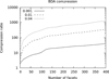 |
Fig. 6 Compression ratios achieved with baseline-dependent averaging, as a function of facet number (thus facet size), for several different decorrelation levels, for a VLA B-configuration observation. |
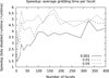 |
Fig. 7 Gridding speedup factors achieved with baseline-dependent averaging, as a function of facet number (thus facet size), for several different decorrelation levels. Observation configuration as per previous figure. |
 |
Fig. 8 Deconvolved images for the simulated data-set described in Sect. 6. The left panel shows the restored image not taking the beam into account and not using wideband deconvolution. Central panel shows the result of the deconvolution taking DDE into account, but still not enabling wideband deconvolution. right panel shows the deconvolution result using ssdga. |
5.3 Sparsification
Recent developments in compressive sensing (CS) theory (see, e.g., Carrillo et al. 2012, and references therein) have provided new mathematical insights into imaging and deconvolution. In particular, CS shows that sparse signals, i.e. signals with limited support in some dictionary, can be successfully recovered from a much smaller number of measurements than that required by e.g. Nyquist sampling, provided a few mathematical criteria (in particular, the Restricted Isometry Property, or RIP) are met. Traditional CLEAN has been shown to be a variation of a CS algorithm.
When multiple major cycles are performed by a CLEAN-like algorithm (as is necessary for even modestly high dynamic range imaging), the models recovered during early major cycles tend to be extremely sparse. This is simply due to the inherent structure of the radio sky: bright sources are few and far between, so it is quite typical that early major cycles of CLEAN affect only a relatively small number of components. Under these conditions, it directly follows from CS theory that we can discard a random subset of uv-samples in the early major cycles (the randomness of the selection ensures that the RIP is maintained), and still recover the same model components, as long as the image signal-to-noise ratio (S/N) remains sufficiently high.
ddfacet implements this idea as the sparsification feature. The implementation naturally interfaces with the BDA gridder. At each major cycle, a user-specified percentage of visibility blocks (i.e. BDA blocks) is tagged as “unlucky” and omitted from the gridding process entirely. Effectively, the uv-coverage is randomly sparsified by a given factor, without changing the relative sampling density. The gridding loop is therefore accelerated by the same factor. The sparsification factor can be set to decrease in successive major cycles, since, at the very least, the final major cycle should be done on the full data.
What is a reasonable sparsification factor? Consider a typical VLA or MeerKAT L-band observation of several hours’ duration. This will contain 106 –107 time-baseline samples (per each frequency channel), and offer an image dynamic range of, conservatively, 104 (in the presence of very bright sources, this can go to 106 and above).Assuming a major cycle gain of 0.1, the first major cycle will clean down to 1000σ, and the second major cycle to 100σ, where σ is the noise rms. A sparsification factor of 100 will reduce S/N by a factor of 10, with a negligible effect on overall uv-coverage, and with the second major cycle remaining well above the noise floor. (In practice, we find that sparsifying above a factor of 100 is not really useful, since at that point the runtime becomes dominated by I/O rather than gridding.) For 5 major cycles, a typical list of sparsification factors would be 100, 100, 30, 10, 1. This results in very substantial acceleration of the first four major cycles.
5.4 Nonregular tessellation
Since astrophysical flux density is not uniformly distributed over the sky, a reasonable DDE calibration strategy consists of clustering sets of sources together, and estimating time–frequency-antenna dependent Jones matrices in each of those directions. As shown by Williams et al. (2016) and van Weeren et al. (2016), it is necessary in that context to image the residual data in the nonregular spatial domains within which the Jones matrices have been estimated.
ddfacet has the ability to image irregularly tessellated images while using 2D FFTs. This is done by providing it with an arbitrary set of nodes (i.e. facet centers). A Voronoi tessellation is then computed internally to generate a polygon file, where each facet is associated with a unique polygon. An image mask is constructed for each polygon. In order to form the residual image, each facet image is multiplied by its corresponding mask, before being stacked onto the combined residual image. We do the converse operation for the degridding.
5.5 Primary beam models
The present implementation of ddfacet can correct for two classes of DDEs: direction-dependent gain solutions derived from a calibration procedure, and/or a priori known DDEs imposed by the primary beam pattern.
The first class of DDEs is specified as an input list of directions and (frequency-dependent) per-antenna Jones terms associated with that direction. Facets are then determined by the nonregular tesselation procedure described above, and imaging proceeds on a per-facet basis, by applying the correct DDE solution (and primary beam E-Jones, computed at facet center) per facet, as described in Sect. 3. In the absence of DD gain solutions, imaging can be done with primary beam corrections alone. In this case the field of view is split into a user-supplied number of square facets, and the primary beam E-Jones is again computed at each facet’s center.
Two primary beam modes are currently implemented. In FITS mode, the user specifies the primary beam pattern as a set of 8 FITS cubes15 giving the real and imaginary components of the 2 × 2 E-Jones elements, as a function of frequency and direction in the antenna frame. ddfacet then computes parallactic angle rotation, and interpolates the E-Jones value appropriate to each facet’s center, as a function of time and frequency. FITS mode is suitable to describing dish arrays. In LOFAR mode, the primary beam corresponding to a LOFAR station is computed using the LofarStationResponse class.
6 Simulations
In this section we discuss in detail a test case for the framework developed throughout this paper. We simulate a small, semi-realistic, LOFAR LBA data-set. The data consists of an interferometric data-set with 630 baselines (36 LOFAR stations), 2.8 h long, with 5 frequency channels spanning the range 30 to 70 MHz. The station are configured in lba_inner mode (van Haarlem et al. 2013) in order to provide us with the widest field of view. The HPBW is on the order 5.77 degrees at 60 MHz.
The simulated sky consists of ~100 point sources with 50-MHz intrinsic fluxdensities S50 = s1.5 with  Jy, and spectral indices
  , where
  is the uniform distribution. To make the case more difficult yet, we add a bright 104 Jy off-axis source.
Apart from the lba_inner station beam being applied, scalar time-frequency-direction dependent Jones matrices are applied to the predicted visibilities. In particular, the Jones matrices have a random phase and amplitude term that varies sinusoidally with time, and this random realization is repeated for each antenna, frequency and direction. The typical amplitude variation is on the level of 0.1, while the phase variation is on the level of 0.1π. This schemeguarantees (i) nonunitarity of the Jones matrices (and Mueller matrices), and (ii) baseline-dependency of the resulting Mueller matrices (see Sect. 3.5).
The Jones matrices together with the LOFAR lba_inner beam are provided to ddfacet and the sky is tessellated as described in Sect. 5.4. The image is 8019 × 8019 pixels with a pixel size of 10 × 10′′, and when the wideband mode is enabled the residual image cube has 3 channels.
To measure the estimated sky produced by the different deconvolution algorithms, we run ddfacet in various modes:
-
[•]di/dd: Direction-independent faceting or direction-dependent faceting.
-
nb/wb: Narrow-band and wideband observations. In the latter case the intrinsic spectral variability is taken into account either by the hmp (hmp-wb) or by the ssdga (ssd-wb).
The results are presented in Figs. 8–10. Figure 8 shows that, as expected, the residuals are much lower when deconvolved with dd+nb and di+wb. In Fig. 9, we plot the relative flux error  as a function of the distance to the beam center. It is quite clear from the plot that, as expected, the di+nb gives biased flux density estimates and higher residual values (see Fig. 8). The main component of the bias is corrected using dd+nb, but the flux density scatter is high. With hmp or ssd deconvolution, the dynamic range increases, and the error on both flux densities and spectral indices decreases. In Fig. 10, we plot the error δα50 in spectral index estimate as a function of the distance from the beam center. While di+wb produces biased spectral index estimates, the hmp or ssd algorithms properly recover them (with ssd doing slightly better).
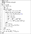 |
Algorithm 3 bda gridder. Here |


 |
Fig. 9 Relative flux density error |

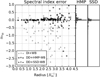 |
Fig. 10 Error |

7 Overview and future work
In this paper we have presented a mathematical framework for wideband wide-field spectral deconvolution that can take generic DDEs into account, as well as an implementation of this framework called the ddfacet imager. This has a number of unique features not available in other imaging and deconvolution frameworks:
-
A wide-field coplanar faceting scheme is implemented. This is a generalization of the Kogan & Greisen (2009) scheme. Nontrivial facet-dependent w-kernels are used to correct for noncoplanarity within the facets.
-
Generic, spatially discrete, time-frequency-baseline-direction-dependent full polarisation Jones matrices can be taken into account in the imaging and deconvolution steps16.
-
As shown in Sect. 3.5 and 3.6, to account for time-frequency-baseline dependent Mueller matrices, we compute a direction dependent PSF for use in the minor cycle of deconvolution.
-
The above also allows for the effects of time and bandwidth averaging to be explicitly incorporated into deconvolution.
In order to accurately deal with large fractional bandwidth of modern interferometers, one has to estimate the spectral properties of the sky term in the Measurement Equation. We have implemented two new wideband deconvolution algorithms:
-
A hybrid matching pursuit algorithm (hmp, see Sect. 4.1), with similarities to mtms-clean (Rau & Cornwell 2011).
-
A hybrid joint deconvolution algorithm that we call Subspace Deconvolution (ssd, see Sect. 4.2). This does joint deconvolution on subsets of pixels (islands), while treating the islands independently. For the former, we have implemented a genetic algorithm to perform the nonlinear optimisation step (Sect. 4.2.2)
Finally, a few interesting and innovative technical features are incorporated:
-
A general tessellation scheme that supports both regular (square) and nonregular (Voronoi tesselation) facets.
-
On-the-fly baseline-dependent averaging within the gridder and degridder, resulting in a factor of several speedup of these operations.
-
A sparsification scheme that dramatically accelerates the initial (shallow) major cycles, when using a CLEAN-style deconvolution loop.
-
Completely asynchronous multiprocessing, which does I/O and computation concurrently, and achieves excellent scaling properties on NUMA architectures.
The current version of ddfacet can deal with full polarisation deconvolution, and can take into account externally defined Jones matrices and/or beam patterns. It has been successfully tested with data diverse telescopes such as LOFAR, VLA, MeerKAT AR1 and ATCA.
Further development of ddfacet is proceeding in a number of directions. These include (i) extending the basis set of ssdga and hmp with Gaussian components for better deconvolution of extended emission, (ii) implementing other types of ssd algorithms, using convex solvers for the optimisation steps, (iii) implementing CS-derived minor cycle algorithms, (iv) back-porting existing multiscale CLEAN algorithms into the framework. On the more technical side, we are working on incorporating (v) GPU-based gridders and degridders, and (vi) the accelerated Direct Fourier Transform implemented in montblanc (Perkins et al. 2015) for high dynamic range imaging. Finally, a distributed implementation of the framework is being designed.
Acknowledgements
The research of O. Smirnov is supported by the South African Research Chairs Initiative of the Department of Science and Technology and National Research Foundation. MJH acknowledges support from the UK Science and Technology Facilities Council [ST/M001008/1]; some testing of ddfacet was carries out using the LOFAR-UK computing facility located at the University of Hertfordshire and supported by STFC [ST/P000096/1]. TWS acknowledges support from the ERC Advanced Investigator program NewClusters 321271.
References
- Bhatnagar, S., Cornwell, T. J., Golap, K., & Uson, J. M. 2008, A&A, 487, 419 [Google Scholar]
- Bhatnagar, S., Rau, U., & Golap, K. 2013, ApJ, 770, 91 [NASA ADS] [CrossRef] [Google Scholar]
- Bridle, A. H., & Schwab, F. R. 1999, in Synthesis Imaging in Radio Astronomy II, eds. G. B. Taylor, C. L. Carilli, & R. A. Perley, ASP Conf. Ser., 180, 371 [Google Scholar]
- Carrillo, R. E., McEwen, J. D., & Wiaux, Y. 2012, MNRAS, 426, 1223 [NASA ADS] [CrossRef] [MathSciNet] [Google Scholar]
- Cornwell, T. J. 2008, IEEE J. Sel. Top. Signal Process., 2, 793 [Google Scholar]
- Cornwell, T. J. & Perley, R. A. 1992, A&A, 261, 353 [NASA ADS] [Google Scholar]
- Cornwell, T. J., Golap, K., & Bhatnagar, S. 2008, IEEE J. Sel. Top. Signal Process., 2, 647 [Google Scholar]
- Cotton, W. D. 1989, in Synthesis Imaging in Radio Astronomy, 6, 233 [NASA ADS] [Google Scholar]
- Cotton, W. 1999, in Synthesis Imaging in Radio Astronomy II, 180, 357 [NASA ADS] [Google Scholar]
- Dabbech, A., Ferrari, C., Mary, D., et al. 2015, A&A, 576, A7 [NASA ADS] [CrossRef] [EDP Sciences] [Google Scholar]
- Fortin, F.-A., De Rainville, F.-M., Gardner, M.-A., Parizeau, M., & Gagné, C. 2012, J. Mach. Learn. Res., 13, 2171 [Google Scholar]
- Garsden, H., Girard, J. N., Starck, J. L., et al. 2015, A&A, 575, A90 [NASA ADS] [CrossRef] [EDP Sciences] [Google Scholar]
- Hamaker, J. P., Bregman, J. D., & Sault, R. J. 1996, A&AS, 117, 137 [NASA ADS] [CrossRef] [EDP Sciences] [Google Scholar]
- Jacob, J. C., Katz, D. S., Prince, T., et al. 2004, The montage architecture for grid-enabled science processing of large, distributed datasets (Pasadena, CA: Jet Propulsion Laboratory, NASA [Google Scholar]
- Kazemi, S., Yatawatta, S., Zaroubi, S., et al. 2011, MNRAS, 414, 1656 [NASA ADS] [CrossRef] [Google Scholar]
- Kogan, L., & Greisen, E. W. 2009, Faceted imaging in AIPS, Tech. Rep. 113, (National Radio Astronomy Observatory. Associated Universities, Inc.) [Google Scholar]
- Noordam, J. E., & Smirnov, O. M. 2010, A&A, 524, A61 [NASA ADS] [CrossRef] [EDP Sciences] [Google Scholar]
- Offringa, A. R., McKinley, B., Hurley-Walker, N., et al. 2014, MNRAS, 444, 606 [NASA ADS] [CrossRef] [Google Scholar]
- Perkins, S. J., Marais, P. C., Zwart, J. T. L., et al. 2015, Astron. Comput., 12, 73 [NASA ADS] [CrossRef] [Google Scholar]
- Rau, U., & Cornwell, T. J. 2011, A&A, 532, A71 [NASA ADS] [CrossRef] [EDP Sciences] [Google Scholar]
- Smirnov, O. M. 2011, A&A, 527, A106 [NASA ADS] [CrossRef] [EDP Sciences] [Google Scholar]
- Smirnov, O. M., & Tasse, C. 2015, MNRAS, 449, 2668 [NASA ADS] [CrossRef] [Google Scholar]
- Tasse, C. 2014a, ArXiv e-prints [arXiv:1410.8706] [Google Scholar]
- Tasse, C. 2014b , A&A, 566, A127 [NASA ADS] [CrossRef] [EDP Sciences] [Google Scholar]
- Tasse, C., van der Tol, S., van Zwieten, J., van Diepen, G., & Bhatnagar, S. 2013, A&A, 553, A105 [NASA ADS] [CrossRef] [EDP Sciences] [Google Scholar]
- Thompson, A. R., Moran, J. M., & Swenson, Jr., G. W. 2001, Interferometry and Synthesis in Radio Astronomy, 2nd edn. (New York: Wiley [CrossRef] [Google Scholar]
- van Haarlem, M. P., Wise, M. W., Gunst, A. W., et al. 2013, A&A, 556, A2 [NASA ADS] [CrossRef] [EDP Sciences] [Google Scholar]
- van Weeren, R. J., Williams, W. L., Hardcastle, M. J., et al. 2016, ApJS, 223, 2 [NASA ADS] [CrossRef] [Google Scholar]
- Williams, W. L., van Weeren, R. J., Röttgering, H. J. A., et al. 2016, MNRAS, 460, 2385 [NASA ADS] [CrossRef] [Google Scholar]
- Yatawatta, S. 2013, Exp. Astron., 35, 469 [NASA ADS] [CrossRef] [Google Scholar]
Throughout the paper, we use the terms stations and antennas interchangably to refer to the elements of an interferometer.
ddfacet is an imager, implemented in C and Python. It will be made publicly available shortly after the publication of this paper.
In practice the gridder and degridder of ddfacet works on Stokes quantities that can be constructed from measured visibilities.
A Mueller matrix proper operates on Stokes vectors rather than visibility vectors. The Mueller matrix in this case would be given by
 , where
S is the
4 × 4
conversion matrix mapping Stokes vectors to visibility vectors. See for example Hamaker et al. (1996); Smirnov (2011).
, where
S is the
4 × 4
conversion matrix mapping Stokes vectors to visibility vectors. See for example Hamaker et al. (1996); Smirnov (2011).
This can be motivated as follows: for any given matrix
A, the null
spaces  and
and
 are identical. Therefore,
applying the adjoint operator
are identical. Therefore,
applying the adjoint operator  to go back to images from visibilities preserves all information not destroyed by
 .
.
In ddfacet the data is internally imaged into frequency-chunked spectral cubes, and the correction described here (Eq. (30)) is done on a user-defined but ideally small bandwidth.
In an abuse of language we can also call inverting  a deconvolution problem, although strictly speaking it is not a convolution operator.
In contrast to a basis, the decomposition of a vector in these dictionaries is not necessarily unique.
Although clean was written before compressive sampling theory had been described.
 is
done computationally by degridding.
is
done computationally by degridding.
Decorrelation is produced by averaging of complex-valued Jones matrices. It is easy to see, for instance, that averaging a rotating complex scalar will result in a loss of amplitude.
In principle it should also be possible to specify a different pattern per antenna, although this option is currently not exposed in the interface.
This is not the case for Bhatnagar et al. (2008); Tasse et al. (2013) that are using A-projection and that need (i) spatially smooth DDE effects, and (ii) time-frequency-baseline independent Jones matrices for the PSF to be direction-independent.
All Tables
All Figures
|
Fig. 1 Comparison between the true δni term, and the first-order approximation (right), and residuals (left). The Kogan & Greisen (2009) approximation breaks down away from the facet center (labeled as uv-scaling, dotted line). Applying classical W-projection together with a Kogan & Greisen (2009) style coordinate transformation works better (dashed line), but a blind 3rd–5th-order polynomial works best (solid line). |
| In the text | |
|
Fig. 2 The nonunitary Mueller matrices in |
| In the text | |
|
Fig. 3 PSF estimated at various locations of the image plane even after the transformation described in Eq. (30) is applied. The net local convolution function significantly varies, and this effect is taken into account by computing a PSF per facet. |
| In the text | |
|
Fig. 4 Residual data for a fraction of the field of view of the simulation described in Sect. 6. The left to right and top to bottom panels show the iterations {0, 1, 2, 3}. As explained in Sect. 4.2.1, the ssd algorithm works differently from a matching pursuit in that it does joint deconvolution on subsets of pixels, and the estimated flux is fully removed at each iteration. The ssd has remarkable convergence properties. |
| In the text | |
|
Algorithm 1 hmp deconvolution algorithm. Here t is a user defined flux density threshold, α is a minor cycle loop gain. Other symbols are defined in Table 1 and/or in the main text. |
| In the text | |
|
Algorithm 2 ssd deconvolution algorithm. Here t is a user defined flux density threshold. |
| In the text | |
|
Fig. 5 Speedup factor (in terms of overall wall time) obtained by running ddfacet on multiple cores. The solid line corresponds to fixed affinities (each worker process was pinned to a single CPU core), while the dashed line to no affinities (the OS scheduler was allowed to migrate processes across cores). In the former case, processes 0–7 were pinned to the first physical CPU, and 8–15 to the second CPU. This explains the slightly better performance in the no-affinities regime with ≤8 processes, as the OS scheduler was allowed to make use of the second CPU. The graph also shows significanly worse scaling in the hyperthreaded regime. |
| In the text | |
|
Fig. 6 Compression ratios achieved with baseline-dependent averaging, as a function of facet number (thus facet size), for several different decorrelation levels, for a VLA B-configuration observation. |
| In the text | |
|
Fig. 7 Gridding speedup factors achieved with baseline-dependent averaging, as a function of facet number (thus facet size), for several different decorrelation levels. Observation configuration as per previous figure. |
| In the text | |
|
Fig. 8 Deconvolved images for the simulated data-set described in Sect. 6. The left panel shows the restored image not taking the beam into account and not using wideband deconvolution. Central panel shows the result of the deconvolution taking DDE into account, but still not enabling wideband deconvolution. right panel shows the deconvolution result using ssdga. |
| In the text | |
|
Algorithm 3 bda gridder. Here |
| In the text | |
|
Fig. 9 Relative flux density error |
| In the text | |
|
Fig. 10 Error |
| In the text | |
Current usage metrics show cumulative count of Article Views (full-text article views including HTML views, PDF and ePub downloads, according to the available data) and Abstracts Views on Vision4Press platform.
Data correspond to usage on the plateform after 2015. The current usage metrics is available 48-96 hours after online publication and is updated daily on week days.
Initial download of the metrics may take a while.