| Issue |
A&A
Volume 611, March 2018
|
|
|---|---|---|
| Article Number | A45 | |
| Number of page(s) | 11 | |
| Section | Extragalactic astronomy | |
| DOI | https://doi.org/10.1051/0004-6361/201730741 | |
| Published online | 22 March 2018 | |
Search for γ-ray emission from superluminous supernovae with the Fermi-LAT
1
Sorbonne Universités, UPMC Univ. Paris 6 et CNRS, UMR 7095, Institut d’Astrophysique de Paris,
98bis bd Arago,
75014
Paris, France
e-mail: This email address is being protected from spambots. You need JavaScript enabled to view it.
, This email address is being protected from spambots. You need JavaScript enabled to view it.
2
Laboratoire AIM-Paris-Saclay, CEA/DSM/IRFU, CNRS, Université Paris Diderot,
91191
Gif-sur-Yvette, France
3
Astronomy Department, University of Geneva,
Ch. d’Ecogia 16,
1290
Versoix, Switzerland
4
GRAPPA Institute, University of Amsterdam,
1098 XH
Amsterdam, The Netherlands
Received:
7
March
2017
Accepted:
25
August
2017
Abstract
We present the first individual and stacking systematic search for γ-ray emission in the GeV band in the directions of 45 superluminous supernovae (SLSNe) with the Fermi Large Area Telescope (LAT). No excess of γ-rays from the SLSN positions was found. We report γ-ray luminosity upper limits and discuss the implication of these results on the origin of SLSNe and, in particular, the scenario of central compact object-aided SNe. From the stacking search, we derived an upper limit at 95% confidence level to the γ-ray luminosity (above 600 MeV) Lγ < 9.1 × 1041 erg s−1 for an assumed E−2 photon spectrum for our full SLSN sample. We conclude that the rate of the neutron stars born with millisecond rotation periods P ≲ 2 ms and B ~ 1012−13 G must be lower than the rate of the observed SLSNe. The luminosity limits obtained on individual sources are also constraining: in particular, SN2013fc, CSS140222, SN2010kd, and PTF12dam can only be born with millisecond periods if B ≲ 1013 G.
Key words: gamma rays: general / supernovae: general
© ESO 2018
1 Introduction
Superluminous supernovae (SLSNe) constitute a rare class of bright transients with luminosities ten to hundreds of times those of usual core-collapse or thermonuclear supernovae (Quimby 2012). With the advent of systematic transient surveys such as the Palomar Transient Factory (Rau et al. 2009), Pan-STARRS1 (Kaiser et al. 2010), Catalina Real-Time Transient Survey (Drake et al. 2009a), or La Silla QUEST (Baltay et al. 2013), optical observations of a large number of these events have been collected, spanning redshifts from z ~ 0.1 to 4 (Cooke et al. 2012). However, the origin of these explosions is not yet understood. Mainly three scenarios have been proposed to explain these exceptionally luminous light curves, which could be (i) powered by the interaction of the supernova (SN) ejecta with the circumstellar medium (e.g. Ofek et al. 2007; Quimby et al. 2011c; Chevalier & Irwin 2011), (ii) pair-instability driven (Gal-Yam et al. 2009; Gal-Yam & Leonard 2009), or (iii) neutron-star driven (Kasen & Bildsten 2010; Dessart et al. 2012; Kotera et al. 2013; Metzger et al. 2014; Murase et al. 2015; Suzuki & Maeda 2017). Given the variety of observed spectra, it is plausible that different processes are at play in different objects (e.g. Gal-Yam 2012a; Nicholl et al. 2014). Interestingly, scenarios (i) and (iii) predict bright associated γ-ray emission in the GeV to TeV range (Murase et al. 2011, 2014, 2015; Katz et al. 2012; Kotera et al. 2013). The search for such γ-ray emission with the Fermi Large Area Telescope (LAT) data is the scope of this paper.
In the most conventional model (scenario i) SLSNe are powered by the interaction between the SN ejecta and a massive, optically thick circumstellar medium (Smith & McCray 2007; Smith et al. 2008; Miller et al. 2009; Benetti et al. 2014). SN2003ma and SN2006gy for example seem to be explained well by this phenomenology (Smith & McCray 2007; Ofek et al. 2007; Smith et al. 2010). Several authors (Murase et al. 2011, 2014; Katz et al. 2012) have demonstrated that a collisionless shock could then be formed and would host efficient cosmic-ray acceleration leading to non-thermal emission from radio-submillimeter to γ-rays. In the GeV range, this emission can escape from the system without severe attenuation, for specific shock velocities (about 4500–5000 km s−1) (Murase et al. 2015), and at late times after the shock breakout. Ackermann et al. (2015) searched for this specific radiation with the LAT at the location of core-collapse SNe (Types IIn and Ib), with standard luminosity, spanning typical time windows of a few months to a year starting from the optical luminosity peak. No detection was reported and model-independent flux upper limits were derived. A fast-rotating central neutron star releasing its rotational energy into the SN ejecta could also drive SLSNe (model iii; e.g. Kasen & Bildsten 2010). The rotation period has to be close to milliseconds to transfer significant energy to the ejecta. The strength of the initial dipole magnetic field of the star sets the timescale over which the energy is injected (a stronger field leads to faster decline). Magnetars (B ~ 1015 G) have thus been proposed as central engines for SLSNe (Kasen & Bildsten 2010; Dessart et al. 2012). Pulsars with millisecond periods at birth and milder dipole magnetic fields B ~ 1013 G would also lead to bright peaks as well as a high-luminosity plateau lasting for several months to years (Kotera et al. 2013; Murase et al. 2015). These authors further calculated that the young neutron-star wind nebula would present a bright X-ray and γ-ray peak, respectively, through synchrotron radiation and inverse Compton (IC) scattering, appearing a few months to years after the explosion. As in model (i), the γ-ray flux would be attenuated above TeV energies owing to two-photon attenuation processes, but is expected to be particularly high around ~10 GeV (Murase et al. 2015).
We present in this work the first systematic individual and stacking search for γ-ray emission in the GeV band, with the LAT, in the directions of 45 SLSNe. We first present the SLSNe sample, dataset, and methods used to measure the γ-ray flux from the directions of selected SLSNe through individual and stacking analyses. We report the γ-ray luminosity upper limits obtained from measurements and discuss the implication of these results on the origin of SLSNe and, in particular, the scenario of a central compact object-aided SN.
2 Superluminous supernovae sample
SLSNe reach typical optical luminosities of ~ 1042–1045 erg s−1 (Quimby et al. 2011c). The γ-ray peak luminosity could be of the same order around the peak energy ϵ ~ 10 GeV (Murase et al. 2015), implying that these objects could be observed with the LAT at a given energy ϵ up to distances Dmax,ϵ = [Lγ,ϵ ∕ (4πFLAT,ϵ)] 1∕2, where Lγ,ϵ is the source γ-ray luminosity and FLAT,ϵ the sensitivity ofthe LAT1 for Pass 8 (Atwood et al. 2013), which are both calculated at energy ϵ. In particular,
 (1)
(1)
The above luminosity distance corresponds to a redshift z ~ 0.36. We selected 45 SLSNe listed in Table A.1 among which 25 are located below this limit. Figure 1 presents the maximum observable distances with the LAT as a function of the source luminosity for different energies ϵ.
In principle, as discussed in Sect. 6, scenarios (i) and (iii) predict γ-ray luminosities that are at least a factor 1/20 to 1/15 lower than the bolometric radiated luminosity. It thus seems more reasonable to look for sources with maximum luminosities of order Lγ ~ 1044 erg s−1 within redshifts z ≲ 0.2. For completeness, we still include the more distant sources in our systematic search. We consider a full sample and two subpopulations bounded by the redshift values 0.0, 0.2, and 1.6.
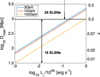 |
Fig. 1 Maximum distance Dmax and corresponding redshift z at which the LAT can observe a SLSN as a function of the γ-ray luminosity Lγ,ϵ, for three energies: ϵ = 3, 10, and 100 GeV. The subsample boundaries are overplotted in black. |
3 Fermi-LAT observations
The LAT, the main instrument on the Fermi spacecraft, is a pair-conversion telescope that is sensitive to γ-rays from 20 MeV to >300 GeV with on-axis effective area >1 GeV of ~ 8000 cm2. The LAT is made of a high-resolution silicon tracker, a hodoscopic CsI electromagnetic calorimeter and an anti-coincidence detector for charged particle background identification. The full description of the instrument and its performance can be found in Atwood et al. (2009). The LAT field of view (~ 2.4 sr) covers the entire sky every 3 h (two orbits) in the survey mode used for this work. The single-event point spread function (PSF) strongly depends on both the energy and conversion point in thetracker, but less on the incidence angle. For 1 GeV normal incidence conversions in the upper section of the tracker the PSF 68% containment radius is 0.6°. Timing is provided to the LAT by the satellite GPS clock and photons are timestamped to an accuracy better than 300 ns. The photons detected by the LAT are categorized in classes according to the energy, direction reconstruction quality, and residual background rates. The categories have different respective strengths depending on the type of analysis (transient, point source, and diffuse emission).
We used for our analysis the Pass 8 LAT data (Atwood et al. 2013), which was collected starting 2008 August 4 and extending until 2015 September 10. This dataset encompasses 7 years and 1 week of observations. There are six main classes within the Pass 8 event reconstruction strategy with the classes nested2 . We selected photons from the “Source” class, which is the third event set in terms of residual charged-particle background and is mainly dedicated to the study of point sources. We kept photons within a radius of 16° from the source position and excluded the periods when the source was viewed at zenith angles > 100° to minimize contamination by photons generated by cosmic-ray interactions in the atmosphere of the Earth. Only photons within the energy range of 600 MeV to 600 GeV were selected. We performed the analyses in seven energy bands between 0.612 and 600 GeV and in the full energy range. Table 1 reports the energy bands used. The energy boundaries are determined by the energy binning of the LAT Collaboration diffuse model3 (Acero et al. 2016a). We chose to use the same binning in our analysis. However to increase photon statistics in particular at the highest energies, we merged the diffuse model energy bands to obtain the larger energy ranges used in our study. Theoretical models (Murase et al. 2015) predict a rather flat spectrum that is consistent with a spectral index of ~ − 2 and owing to the poor angular resolution at low energy (50–600 MeV), we do not expect photons at those energies to contribute significantly to our sensitivity.
Energy band boundaries.
4 Analysis
4.1 Analysis by maximum likelihood estimator (MLE)
4.1.1 Individual analysis
The analysis method is similar to that described in Renault-Tinacci et al. (2015). We describe the main steps below. The spectral analysis was carried out in the energy bands listed in Table 1. We test both wide and narrower energy bands to observe the impact of the increase of photon statistics and of a better sampling of the source spectrum. We modelled the γ-ray emission in an 18° × 18° square region centred on the position of each source. The model consists of a linear combination of a point source at the SN position and of template maps for the diffuse interstellar emission and the isotropic flux resulting from the extragalactic γ-ray background and residuals due to cosmic rays misclassified as γ-rays. The interstellar component and isotropic spectra are available at the Fermi Science Support Centre4 . The model also includes all point sources and extended sources listed in the 3FGL catalogue (Acero et al. 2015).
The γ-ray intensity in each (l, b) direction in Galactic coordinates, I(l, b, E) in cm−2 s−1 sr−1 MeV−1, is modelled at each energy E as
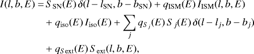 (2)
where SSN(E) gives the source spectrum in cm−2 s−1 MeV−1 and the IISM(l, b, E) and Iiso(E) terms denote the interstellar and isotropic intensities in cm−2 s−1 sr−1 MeV−1, respectively. The qISM(E) and qiso(E) parameters are simple normalization factors to account for possible deviations from the two input spectral shapes.
(2)
where SSN(E) gives the source spectrum in cm−2 s−1 MeV−1 and the IISM(l, b, E) and Iiso(E) terms denote the interstellar and isotropic intensities in cm−2 s−1 sr−1 MeV−1, respectively. The qISM(E) and qiso(E) parameters are simple normalization factors to account for possible deviations from the two input spectral shapes.
Depending on the latitude of the analysis region, the number of background sources in the region varied from 7 to 27 with an average number around 12. We used the source flux spectra Sj(E) from the catalogue as input spectra for the sources (in cm−2 s−1 MeV−1). Their individual flux normalizations  have been let free in each energy band to compensate for potential deviations between the 4-year long observations of the catalogue and our extended dataset.
We modelled the γ-ray intensity inside the analysis region and in a 7°-wide peripheral band to account for photons spilling over inside the analysis region because of the wide LAT PSF. The contribution from the sources detected in the outer band has been summed into a single map Sext(l, b, E) and its normalization  has been left as a free parameter (Ade et al. 2015).
The model intensity I(l, b, E) has been processed through the LAT instrument response functions (IRFs, P8R2_V6SOURCE) to take into account the position-dependent and energy-dependent exposure on the sky and the energy-dependent PSF. We calculated the effective IRFs for the spectrum of each component, taking a power-law spectrum with a photon index equal to − 2 as spectral input for the studied SLSNe. An example of a model sky map is presented in Fig. 2 for SN2013fc.
The modelled photon map, integrated over each energy band, can be compared to the observed data by means of a binned MLE with Poisson statistics to fit the model coefficients to the LAT data (Anderson et al. 2015). We stress that the present analysis independently fits the source flux in each energy band and that it is independent of the initially assumed spectral shape.
To quantify the detection significance of the emission, we used the test statistic, ![Mathematical equation: $TS = 2 \left[\ln(L)-\ln(L_0)\right]$](/articles/aa/full_html/2018/03/aa30741-17/aa30741-17-eq5.png) , where L0 and L are the maximum-likelihood values obtained for the null hypothesis (zero flux from the SN) and when a point source at SN position is assumed, respectively. In the first (and fairly robust) approximation in case of a difference of 1 degree of freedom, the significance is equal to the square root of the TS. We set a detection threshold above a TS of 25, i.e. a 5σ significance.
, where L0 and L are the maximum-likelihood values obtained for the null hypothesis (zero flux from the SN) and when a point source at SN position is assumed, respectively. In the first (and fairly robust) approximation in case of a difference of 1 degree of freedom, the significance is equal to the square root of the TS. We set a detection threshold above a TS of 25, i.e. a 5σ significance.
Performing multiple analysis trials with different parameters, as we have here with several SLSNe for instance, introduces a bias in the analysis due to the so-called look-elsewhere effect (Choudalakis 2011). The chance that the observed significance could have arisen at random due to the size of the parameter space that was searched can be accounted for by applying trials factor corrections to the final significance. For the individual search study, we have to consider 45 SLSNe, seven individual and independent energy bands, the total energy range that overlaps the individual bands, and five overlapping time windows. This corresponds to a number of trials Ntrials = 1800. For such a high number of trials, a 5σ (4σ) pre-trial detection would correspond to a 3.3σ (1.6σ) significance after trials correction. The best significance, obtained for SN2012il in the 3-month time window and the 67–172 GeV band, is equal to 3.8σ, which is decreased to 1.2σ after applying the trials factor. This correction assumes that each dataset is statistically independent, which is overly conservative in our case, since four of the five time windows result in datasets that are subsets of each other and the total energy range overlaps the individual energy bands. Therefore we regard the final detection significances as conservative lower limits to the true significances of the signal over the background.
We checked the existence of a steady γ-ray source in the direction of the selected SLSNe. Such a source could be the host galaxy of the SN or a source along the line of sight. In case of detection (TS > 25, significance > 5σ), a new source would be added to the catalogued sources at the position of the SLSN. We searched for γ-ray emission in the SLSN off-peak dataset, i.e. either between the first available γ-ray observations (2008 August 8) and 1 month before the presumed date of the SN peak time, tSN , or for three SLSNe (SN2008fz, SN2009jh, and PTF09atu) the two last years before the end of the exploited dataset (2015 September 10) because their peak time is less than 1 year after the observations start. No significant source was found in the SN directions in the off-peak window. The existence of significantγ-ray emission from the host galaxy or an aligned source would make the detection of a faint SN signal more difficult.
Theoretical simulations of the duration of the γ-ray emission predict γ-ray emission lasting weeks to months depending on the SN and the central compact object characteristics (Murase et al. 2015). Hence this prediction motivates a search in several time windows. Individual and joint likelihood analyses were performed for the following observation periods:
-
from tpeak5 − 1 month (referred to as tSN in the next sections) up to tpeak + 3 months;
-
from tpeak − 1 month up to tpeak + 6 months;
-
from tpeak − 1 month up to tpeak + 1 year;
-
from tpeak − 1 month up to tpeak + 2 years.
Only 44, 40, and 33 SNe were studied for the 6-month, 2- and 1-year time windows, respectively, because the available dataset was too short for the needed duration. On the other hand, all sources were analysed for the 3-month time windows. To make sure no early γ-ray emission was missed, we used datasets starting 30 days before the optical peak time to account for the uncertainty in its determination (Cano et al. 2015; Liu et al. 2017).
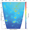 |
Fig. 2 Source model map of SN2013fc after fit integrated over the 600 MeV–10 GeV energy band. The red cross points to the position of the SN2013fc. The thin red line indicates the boundary between the inner map where sources are independently fitted and the peripheral band where the contribution from all sources is fitted as one. All other sources, included in the source model map were previously detected with the Fermi-LAT and their fluxes were fitted during the procedure. |
4.1.2 Joint likelihood analysis
To improve the sensitivity of the analysis to a weak γ-ray signal from SLSNe, we combined sources in a joint likelihood analysis (Anderson et al. 2015). We studied the complete sample and split it into two subgroups based on redshift (and hence also on distance). Figure 1 summarizes the repartition of studied SLSNe. Some sources exploded late with respect to the dataset time limits preventing us from including these sources into the joint likelihood analysis for the longer time bins. Only the 3-month analysis includes the complete sample. Otherwise, we used sources from SN2008fz to DES13S2cmm, SN2008fz to PS1-14bj, and SN2008fz to SN2015bn for the 2-year, 1-year, and 6-month analyses, respectively (following the order in Table A.1).
To be independent from any spectral shape assumption we performed the analysis in energy bands (see Sect. 4.1.1 for details). We performed the combined analysis by tying together in each energy band the flux normalization of all SLSNe in the subsample (Ackermann et al. 2015). It results in a single free parameter per energy band. To correctly tie the SN normalizations together, we defined a common γ-ray scaling factor; i.e. we give more weight to sources with greater expected γ-ray flux in the joint likelihood. Two different weighting approaches can be envisaged in the stacking procedure, relying either on the optical flux or the luminosity distance. Considering the difficulties in concatenating a consistent set of optical magnitude values for the whole sample, we ruled out the optical flux approach. For the joint analysis we assumed all SLSNe to have the same intrinsic γ-ray luminosity and thus the observed γ-ray flux of each source scales with a factor inversely proportional to the luminosity-distance squared. The weight of the flux normalization of each source in each energy bin is  .
.
We derived the SLSNe distances from redshift measurements and a set of cosmological parameters from the Λ CDM model. We used H0 = 69.6 km s−1 Mpc−1, Ω M = 0.286, and ΩΛ = 0.714 values provided in Ade et al. (2016) but other sets exist. Hence we calculated roughly that the choice of a different set would resultin distance estimates less than 5% greater or lower with other commonly used cosmological parameters (e.g. Ade et al. 2014; Hinshaw et al. 2013; Nicholl et al. 2014; Benetti et al. 2014).
For the joint likelihood analysis, only the SN normalization is free in each energy band while the nearby source, diffuse, and isotropic component normalizations are fixed to their values obtained in the individual analyses of each source in the corresponding energy band.
Identically to the individual searches, many trials are realized for the joint likelihood analysis. We count here four time windows, seven small energy bands and the total range, and two redshift subpopulations and the full sample, which brings us to Ntrials = 96. Again the correction is conservative as the redshift subsets overlap along with the time windows and total energy range. In this case, a 5σ, 4σ, or 3σ significance would correspond to a 4σ, 2.7σ, or 1.2σ post-trial detection level, respectively. With the total SLSN population, the 2-year time window and in the 67–172 GeV band, a 3.8σ significance is obtained and is decreased to 2.4σ after trials factor correction. We thus report only upper limits.
4.2 Aperture photometry
We independently verified the results of the likelihood analysis using the aperture photometry method for spectral extraction. For the aperture photometry, we extracted the source signal from circular regions of radius 1° around each source listed in Table A.1. Photons of the “Source” class were retained for the analysis. For each source region the exposure was calculated using the gtexposure tool, which accounts for the energy-dependent loss of the source signal due to the large size of the LAT PSF extending beyond the 1° around the source position energies.
The background was estimated from source-free regions of radius 3° within <10° distance from the source position. This assures that the level of the Galactic diffuse background in the source and background estimate regions is similar. The level of the Galactic diffuse background varies on different angular scales. This is the main limitation of the aperture photometry method, especially for the sources close to the Galactic Plane. However, most of the sources considered for the stacking analysis are at high Galactic latitudes where the level of variations of the Galactic diffuse emission is more moderate and their angular scale is typically larger than a few degrees. This justifies the use of the aperture photometry as a cross-checking method.
The two analysis methods are complementary in the sense that the aperture photometry provides a robust upper limit on the luminosity, which is independent of the details of modelling of diffuse backgrounds in the source region of interest. At the same time, the (moderately) model-dependent likelihood analysis allows us to tighten the upper limits on the luminosity of the SLSN source sample.
5 Results
In the following section, we report the upper limits at 2σ confidence on the summed luminosities, 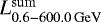 and
and  . These are the sum of measured luminosities in the individual energy bands located between the indicated energy boundaries. These luminosities are named this way in contrast to the total luminosity obtained directly by fitting the flux in the studied energy band. On the other hand, the summed luminosity is the sum of the fluxes obtained by fitting fluxes separately in narrow energy bins covering the large energy band and summing them afterwards. The second method via summation allows us to reach a better sampling of the actual source spectrum compared to the first method through a direct fit that provides a rougher measure of the luminosity. To compute the upper limits on the γ-ray luminosity in individual energy bands from the measured photon fluxes and their errors, we assumed, as for the input spectrum, a E−2 power law in each energy band. We emphasize that the derived upper limits on
  are the most important measurements to probe the theoretical predictions.
5.1 Individual analysis
We gather in Table A.2 the individual luminosities or upper limits at 2σ confidence. No detection, after trial factor correction, are reported over the total energy range nor in individual bands. The only obtained small over-fluctuation occurs in an individual energy band for SN2012il between 67 and 172 GeV at 1.2, 0.9, 0.7, and 0.3σ levels in the 3-month to 2-year time windows, respectively. It is however insignificant. The most constraining upper limit for an individual source was obtained for SN2013fc with a 2-year time window and is equal to 1.2 × 1042 erg s−1 (see Fig. 3).
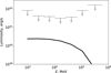 |
Fig. 3 Upper limits on the luminosity of SN2013fc from the individual analysis of the 2-year time window. Down arrows indicate upper limits at 2σ confidence.The black line represents the integrated luminosity computed from a simulated spectrum derived by Murase et al. (2015) for a neutron star with P = 10 ms, B = 1013 G at a distanced = 16.5 kpc and about 206 days after explosion. |
5.2 Jointlikelihood analysis
Tables 2–4 provide the upper limitson luminosity for the stacking analysis obtained for both energy band sets. The study was carried out with three different source samples:
-
all sources;
-
sources with redshift z ∈ [0.0;0.2];
-
sources with redshift z ∈ [0.2;1.6].
Joint likelihood fits result, after trial factor correction, for either of the redshift samples and time windows, in no detection. A 2.4σ over-fluctuation (post trials) can be reported in the 67–172 GeVindividual energy band with the 2-year dataset and the complete sample. The latter includes mostly (~ 66%) sources thatare too distant to be detectable individually and hence we considered this fluctuation as insignificant. Joint likelihood analyses on the subsample of lowest redshifts (closest SLSNe) should be more relevant if any signal was detected. In the absence of signal, i.e. when we are looking at an empty sky, the tightest upper limit is provided by the joint analysis with the largest sample and the longest dataset and is independent of the source distances.
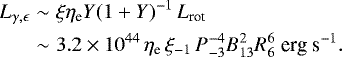
As expected since we do not detect anything but an over-fluctuation, the most constraining limit on the luminosity, Lγ < 9.1 × 1041 erg s−1, is obtained for the total population of SLSNe and the 2-year time window. Figure 4 represents the luminosity upper limits as a function of energy for this case. We obtained upper limits with the subsample for z > 0.2 lower than for z < 0.2 and this is simply explained by the fact that the subset z > 0.2 is larger than the subpopulation with z < 0.2 and both samples result in no detection and hence are basically two empty skies. We considered both close and farthest SLSNe because we simply took into account all the catalogued SNe. Nonetheless we had in mind that those with redshift beyond 0.2 would be theoretically undetectable.
The results of the aperture photometry analysis, shown in Fig. 5 for the 2-year time span, are consistent with those of the likelihood analysis, although the upper limits on the luminosity of the stacked source sample are somewhat higher (by ≃ 30%) in the GeV energy band. At the same time, in the energy range above 100 GeV the aperture photometry bound is tighter than that derived from the likelihood analysis. This is explained by the fact that the background photon statistics in this energy band are low and the signal is detectable in a nearly background-free regime. Modelling of the diffuse background in the likelihood analysis approach introduces additional parametersin the analysis and, as a consequence, slightly relaxes the bounds on the source flux and luminosity. However, modelling the diffuse background precisely is more critical at low energy and for sources close to the Galactic plane. Hence, modifying the diffuse model in this analysis (E > 600 MeV and high latitudes) would only have a tiny effect. Acero et al. (2016b) performed a study of the systematic errors dueto the choice of the diffuse model.
Luminosities from joint likelihood analysis measurements with all sources.
Luminosities from joint likelihood analysis measurements and sources with redshift between 0.2 and 1.6.
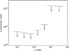 |
Fig. 4 Upper limits on the luminosity of the SLSN from joint likelihood analysis for a 2-year time window and a sample containing all sources (Table 2). Down arrows indicate upper limits at 2σ. |
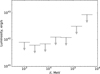 |
Fig. 5 Upper limits on the luminosity of the SLSN obtained from the aperture photometry for a 2-year time window and a sample containing all sources. Down arrows indicate upper limits at 2σ. |
6 Discussion
We discuss here the implication of the derived contraints on the γ-ray luminosity received from SLSNe in the scenario of central compact object-aided SN. In this scenario, a fast-rotating central neutron star releases its rotational energy into the SN ejecta via its wind (see Sect. 1 and see e.g. Kasen & Bildsten 2010; Kotera et al. 2013). The electromagnetic energy of the pulsar is dissipated into kinetic energy in the wind at a yet unknown location (see e.g. Kirk et al. 2009), seeding the surrounding pulsar wind nebula with accelerated pairs. These are expected to radiate by synchrotron or IC scattering and possibly produce a γ-ray emission. The simulations presented in Murase et al. (2015) in this framework were used as a basis for the discussion.
From the upper limits on the γ-ray luminosity measured at the location of SLSNe, it is possible to derive constraints on the values of the central neutron star period P and dipole field strength B.
The emitted γ-ray signal is produced by leptons accelerated in the young neutron star wind nebula region, as is evidenced for example in the Crab nebula and as is successfully modelled in various other pulsar wind nebulae (e.g. Gelfand et al. 2009; Fang & Zhang 2010; Bucciantini et al. 2011; Tanaka & Takahara 2011). The energy channeled into γ-rays should scale as the electromagnetic luminosity provided by the pulsar into the wind6 , 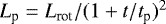 , where the initial pulsar luminosity
  erg s−1, over a typical spin-down timescale tp . The pulsar rotational energy reservoir can be written
  , assuming for simplicity a pulsar spin-down braking index7 n = 3. The spin-down timescale is given by
 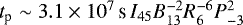 . In all the above formulae, R and I are the star radius and the moment of inertia (see Shapiro & Teukolsky 1983), respectively.
A fraction ηe of Lp is dissipated into pairs at the pulsar wind nebula. The level of this dissipation is currently the subject of intense discussions in the community, and is related to the so-called “sigma-problem” (see e.g. Kirk et al. 2009). However, the observations of the Crab nebula and of other young nebulae point to ηe ~ 1 (e.g. Kirk et al. 2009) with a less significant fraction of the wind energy going into the nebula magnetic field. The pairs then radiate via synchrotron and IC processes in the nebula region, and this emission is attenuated by the radiation fields in the nebula and by matter further out in the supernova ejecta.
In the 1–10 GeV energy range, for observation times of months to a few years after the supernova explosion, the radiation is dominated by the IC process and the obtained spectrum follows approximately a power law of index ~ − 2 (Murase et al. 2014). The expected luminosity of a young neutron star at time tp at energies ϵ ~ 1–10 GeV can then be written (Kotera et al. 2013; Murase et al. 2014) as
 (3)
(3)
Here Y = tsyn∕tIC is the Compton parameter, i.e. the ratio between the synchrotron and IC cooling timescales. The numerical value is calculated assuming a Thomson regime Y = 1. This is a safe estimate as the Klein–Nishina effect mainly cuts off the flux at high energies but does not affect the overall normalization between 1–10 GeV. The factor ξ < 1 takes into account the spread of the IC radiation over a given energy range with the uncertainties on the spectral indices at injection – which can range from hard indices ~−1.5 for reconnection-type, one-shot acceleration processes to softer indices ≲−2 for stochastic acceleration mechanisms – and the attenuation due to radiation and matter. Interestingly, in this energy range, for t ~ tp and for mildly magnetized objects (B ≳ 5 × 10¹³ G), the radiated flux is robust to attenuation by the nebula radiation fields and matter, within a factor of a few (Murase et al. 2015). A value of ξ = 0.1 can thus be viewed as reasonable. However, for magnetars, the radiated spectra are softer and the overall flux are lower and lead to ξ ≪ 1.
Figure 6 shows the contours of the luminosity Lγ,1−10 GeV estimated in the parameter space P − B, assuming ηe = 1 and ξ = 0.1. We overlaid the luminosity limits derived for individual SLSNe for which we obtained the strongest constraints, and for the total stacked sample for time windows of tSN to tSN + 2 years or tSN + 1 year. Table 5 summarizes these upper limits. In the contour plot, the sets of P − B above the line are allowed for a given source or population, modulo the scaling factor ηe ξ−1. In particular within the conservative hypotheses on ηe and ξ−1, the central pulsar can be submillisecond only if B < 2 × 10¹² G. In Figs. 7 to 10 of Murase et al. (2015), two simulated cases for P = 2 ms and P = 10 ms are presented for different magnetic field values. The results presented in this paper rule out the case with P = 2 ms.
The limit given by the joint likelihood analysis of all sources in our sample (white line) places strong constraints on the rate of the neutron star population with mild dipole magnetic fields and millisecond rotation periods. It indicates that the rate of objects born with millisecond-rotation periods P ≲ 2 ms and B ~ 1012−13 G (where the assumption ηe ξ−1 = 1 is conservative) must be lower than the rate of the observed SLSNe (of order ~ 200 Gpc−3 yr−1 at z~ 0.16; Quimby et al. 2013b). The luminosity limits obtained on individual sources are also constraining: in particular, SN2013fc, CSS140222, and SN2010kd can be born with millisecond periods only for B ≲ 1013 G. The derivedupper limit for SN2013fc, the closest source of the sample located at about 80 Mpc, is only ~30% higher than for the joint likelihood analysis (whose reference distance is equal to 100 Mpc) for the same time window. This indicates that the combined limit, obtained with the 1∕d2-weighting, is dominated by the closest source(s). A similar result was noticed in Ackermann et al. (2015).
Ackermann et al. (2015) followed the same method of joint likelihood analysis to search for the emission from standard core-collapse supernovae. They discuss their results within the framework of the model of interaction of the SN ejecta with the circumstellar material. As in this work, weighting for the distances, they derived upper limits on the emitted luminosity. These authors obtain Lγ,1−10 GeV < 2.8 × 1040 erg s−1 compared to Lγ,1−10 GeV < 9.1 × 1041 erg s−1 in our study. Their luminosity constraint is roughly a factor 30 tighter than that measured in this paper, despite a dataset that is a third shorter because they studied a sample more than three times larger and roughly five times closer (hence more detectable).
Our results suppose that the dipole magnetic field of the neutron star is set at its highest value at birth. However some studies (Muslimov & Page 1995; Ho 2011; Viganò & Pons 2012) propose that the fallback accretion after a supernova explosion onto the newborn neutron star would result in the burial of the magnetic field into the crust and its re-emergence over a time scale of thousands years or more (e.g. Geppert et al. 1999; Ho 2011). The diffusion time of the magnetic field, which results in its growth, is strongly dependent on the depth of burial, itself directly related to the mass of accreted matter (Ho 2011; Lorenz et al. 1993). In addition, the mass of accreted matter inversely scales with the space velocity of the neutron star (Güneydaş & Ekşi 2013). Hence according to this model, a runaway neutron star would be more unlikely to have a buried magnetic field. Torres-Forné et al. (2016) showed that masses as low as 10−3 − 10−2 M⊙ are sufficient to bury a few 1012 G magnetic field. This makes the occurrence of such phenomena not unusual and hence must be kept in mind when considering the pulsar-aided scenario.
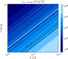 |
Fig. 6 Expected γ-ray luminosities Lγ,1−10 GeV of SLSNe powered by neutron stars with dipole magnetic field B and rotation period P, assuming a pair luminosity fraction ηe = 1 and an attenuation factor ξ = 0.1 (see Eq. (3)). Overlaid are the γ-ray luminosity limits derived in this work for selected individual SLSNe in black lines, and for the total joint likelihood analysis sample as a white line (Table 2), for time windows of tSN to tSN + 2 years or tSN + 1 year for CSS140222. The white dotted line indicates the limit derived for standard core-collapse SNe (Ackermann et al. 2015). The parameter-space above the line is allowed for a given source or population, modulo the scaling factor ηe ξ−1 , with ξ < 1 in any case. The high magnetic field end (B ≳ 5 × 10¹³ G) should be viewed with care as in the magnetar regime, ξ ≪ 1, implying less stringent constraints on the parameter space. |
7 Conclusion
We searched for the first time, through individual and stacking analyses, for γ-ray emission from a reasonable sample of SLSNe discovered through optical surveys. No signals were observed above the detection threshold and we derived the first upper limits on γ-ray signals from these objects. Assuming a scaling of the γ-ray flux with 1∕d2, we report an upper limit at 95% confidence level to the γ-ray luminosity Lγ < 9.1 × 1041 erg s−1 for an assumed E−2 photon spectrum, for our full SLSN sample and the 2-year time window.
Three scenarios are mainly proposed to explain the exceptional luminosities of SLSNe. Two of these scenarios, one relying on the interaction of the supernova ejecta with the circumstellar material and the other on the power supplied by a central compact object, predict γ-ray emission in the GeV–TeV range. Both can apply to SLSNe but also to standard core-collapse SNe.
From the LAT non-detection and the predictions from the neutron-star powered model, one can obtain observational constraints on the rotation period and dipolar magnetic field strength of the central object. Based on conservative assumptions, we find that the rate of the neutron stars born with millisecond rotation periods P ≲ 2 ms and B ~ 1012−13 G must be lower than the rate of the observed SLSNe. The luminosity limits obtained on some individual sources are also constraining.
We recommend reiterating this analysis in the future with a much larger sample of SLSNe (upper limits decreasing as the square root of the number of stacked sources), more γ-ray data and better sensitivity. However it would be really difficult to improve the upper limits by more than a factor 2 or 3. Another approach would be to weight the sources differently, with respect to the optical flux for instance as in Ackermann et al. (2015), if one is able to consistently concatenate a catalogue of optical flux values for a large sample of SLSNe. In any case, future studies of SLSNe will benefit from the upcoming optical surveys that will provide an unprecedently complete catalogue of detailed informations on SNe. The Zwicky Transient Facility (ZTF; first light in 2017, Bellm 2014) and the Large Synoptic Survey Telescope (LSST; under construction in Chile, Abell et al. 2009) will be particularly relevant and efficient.
Luminosities from joint likelihood analysis measurements and sources with redshift between 0.0 and 0.2.
Acknowledgements
We thank K. Murase for fruitful discussions and A. Franckowiak for her careful reading and insightful comments. N.R.T. was supported by the PER-SU fellowship at Sorbonne Universités. K.K. acknowledges financial support from the PER-SU fellowship at Sorbonne Universités and from the Labex ILP (reference ANR-10-LABX-63, ANR-11-IDEX-0004-02). The Fermi-LAT Collaboration acknowledges generous ongoing support from a number of agencies and institutes that have supported both the development and operation of the LAT as well as scientific data analysis. These include the National Aeronautics and Space Administration and the Department of Energy in the United States, the Commissariat à l’Energie Atomique and the Centre National de la Recherche Scientifique/Institut National de PhysiqueNucléaire et de Physique des Particules in France, the Agenzia Spaziale Italiana and the Istituto Nazionale di Fisica Nucleare in Italy, the Ministry of Education, Culture, Sports, Science and Technology (MEXT), High Energy Accelerator Research Organization (KEK) and Japan Aerospace Exploration Agency (JAXA) in Japan, and the K.A. Wallenberg Foundation, the Swedish Research Council and the Swedish National Space Board in Sweden. Additional support for science analysis during the operations phase is gratefully acknowledged from the Istituto Nazionale di Astrofisica in Italy and the Centre National d’Études Spatiales in France. S.A. was supported by NetherlandsOrganization for Scientific Research (NWO) through a Vidi grant. This work performed in part under DOE Contract DE-AC02-76SF00515. We also thank Guillochon et al. (2017) for the useful online catalogue of SN data they set up. The authors wish to acknowledge the anonymous referee for the helpful suggestions and comments that enriched thepaper and helped to highlight some of its results. This work is supported by the APACHE grant (ANR-16-CE31-0001) of the French Agence Nationale de la Recherche.
Appendix A Additional tables
Equatorial and Galactic coordinates, redshift, and SN date in Gregorian and MJD calendars of the studied SLSNe.
Luminosities from measurements between tpeak and tpeak+3 months, 6 months, 1 year, and 2 years.
References
- Abell, P. A., Allison, J., Anderson, S. F., et al. 2009, LSST Science Book, Version 2.0 [arXiv:0912.0201] [Google Scholar]
- Acero, F., Ackermann, M., Ajello, M., et al. 2015, ApJS 218, 23 [Google Scholar]
- Acero, F., Ackermann, M., Ajello, M., et al. 2016a, ApJS 223, 26 [NASA ADS] [CrossRef] [Google Scholar]
- Acero, F., Ackermann, M., Ajello, M., et al. 2016b, ApJS 224, 8 [NASA ADS] [CrossRef] [Google Scholar]
- Ackermann, M., Arcavi, I., Baldini, L., et al. 2015, ApJ 807, 169 [NASA ADS] [CrossRef] [Google Scholar]
- Ade, P. A. R., Aghanim, N., Armitage-Caplan, C., et al. 2014, A&A 571, A16 [NASA ADS] [CrossRef] [EDP Sciences] [Google Scholar]
- Ade, P. A. R., Aghanim, N., Aniano, G., et al. 2015, A&A 582, A31 [NASA ADS] [CrossRef] [EDP Sciences] [Google Scholar]
- Ade, P. A. R., Aghanim, N., Arnaud, M., et al. 2016, A&A 594, A13 [NASA ADS] [CrossRef] [EDP Sciences] [Google Scholar]
- Anderson, B., Chiang, J., Cohen-Tanugi, J., et al. 2015, in 5th Fermi Symp. [arXiv:1502.03081] [Google Scholar]
- Atwood, W. B., Abdo, A. A., Ackermann, M., et al. 2009, ApJ 697, 1071 (LAT Instrument Paper) [NASA ADS] [CrossRef] [Google Scholar]
- Atwood, W., Albert, A., Baldini, L., et al. 2013, in 2012 Fermi Symp. Proc. [arXiv:1303.3514] [Google Scholar]
- Baltay, C., Rabinowitz, D., Hadjiyska, E., et al. 2013, PASP 125, 683 [NASA ADS] [CrossRef] [Google Scholar]
- Bellm, E. 2014, in The Third Hot-wiring the Transient Universe Workshop, eds. P. R. Wozniak, M. J. Graham, A. A. Mahabal, & R. Seaman, 27 [Google Scholar]
- Benetti, S., Nicholl, M., Cappellaro, E., et al. 2014, MNRAS 441, 289 [NASA ADS] [CrossRef] [Google Scholar]
- Benitez, S., Polshaw, J., Inserra, C., et al. 2014, ATel, 6118 [Google Scholar]
- Blagorodnova, N., Campbell, H., Fraser, M., et al. 2014, ATel, 5934 [Google Scholar]
- Bucciantini, N., Arons, J., & Amato, E. 2011, MNRAS 410, 381 [Google Scholar]
- Cano, Z., de Ugarte Postigo, A., Perley, D., et al. 2015, MNRAS 452, 1535 [NASA ADS] [CrossRef] [Google Scholar]
- Cenko, S. B., Kandrashoff, M. T., Silverman, J. M., & Filippenko, A. V. 2010, Central Bureau Electronic Telegrams 2461, 2 [NASA ADS] [Google Scholar]
- Chandra, P., Ofek, E. O., Frail, D. A., et al. 2009, ATel, 2241 [Google Scholar]
- Chevalier, R. A., & Irwin, C. M. 2011, ApJ 729, L6 [Google Scholar]
- Chomiuk, L., Chornock, R., Soderberg, A. M., et al. 2011, ApJ 743, 114 [NASA ADS] [CrossRef] [Google Scholar]
- Choudalakis, G. 2011, Prepared for PHYSTAT2011 [arXiv:1101.0390] [Google Scholar]
- Cooke, J., Sullivan, M., Gal-Yam, A., et al. 2012, Nature 491, 228 [NASA ADS] [CrossRef] [PubMed] [Google Scholar]
- Dessart, L., Hillier, D. J., Waldman, R., Livne, E., & Blondin, S. 2012, MNRAS 426, L76 [NASA ADS] [CrossRef] [Google Scholar]
- Dong, S., Shappee, B. J., Prieto, J. L., et al. 2016, Science 351, 257 [NASA ADS] [CrossRef] [Google Scholar]
- Drake, A. J., Djorgovski, S. G., Mahabal, A., et al. 2009a, ApJ 696, 870 [NASA ADS] [CrossRef] [MathSciNet] [Google Scholar]
- Drake, A. J., Djorgovski, S. G., Mahabal, A., et al. 2009b, Central Bureau Electronic Telegrams, 1958 [Google Scholar]
- Drake, A. J., Djorgovski, S. G., Prieto, J. L., et al. 2010a, ApJ 718, L127 [NASA ADS] [CrossRef] [MathSciNet] [Google Scholar]
- Drake, A. J., Mahabal, A. A., Djorgovski, S. G., et al. 2010b, ATel, 2544 [Google Scholar]
- Drake, A. J., Djorgovski, S. G., Graham, M. J., et al. 2013a, Central Bureau Electronic Telegrams, 3459 [Google Scholar]
- Drake, A. J., Djorgovski, S. G., Mahabal, A., et al. 2013b, Central Bureau Electronic Telegrams, 3560 [Google Scholar]
- Fang, J., & Zhang, L. 2010, A&A 515, A20 [NASA ADS] [CrossRef] [EDP Sciences] [Google Scholar]
- Gal-Yam, A. 2012a, Science 337, 927 [NASA ADS] [CrossRef] [PubMed] [Google Scholar]
- Gal-Yam, A. 2012b, Science 337, 927 [NASA ADS] [CrossRef] [PubMed] [Google Scholar]
- Gal-Yam, A., & Leonard, D. C. 2009, Nature 458, 865 [NASA ADS] [CrossRef] [PubMed] [Google Scholar]
- Gal-Yam, A., Mazzali, P., Ofek, E. O., et al. 2009, Nature 462, 624 [NASA ADS] [CrossRef] [PubMed] [Google Scholar]
- Gelfand, J. D., Slane, P. O., & Zhang, W. 2009, ApJ 703, 2051 [NASA ADS] [CrossRef] [Google Scholar]
- Geppert, U., Page, D., & Zannias, T. 1999, A&A 345, 847 [NASA ADS] [Google Scholar]
- Graham, M. L., Zheng, W., Filippenko, A. V., et al. 2014, ATel, 6635 [Google Scholar]
- Guillochon, J., Parrent, J., Kelley, L. Z., & Margutti, R. 2017, ApJ 835, 64 [NASA ADS] [CrossRef] [Google Scholar]
- Güneydaş A., & Ekşi K. Y. 2013, MNRAS 430, L59 [NASA ADS] [CrossRef] [Google Scholar]
- Hinshaw, G., Larson, D., Komatsu, E., et al. 2013, ApJS 208, 19 [NASA ADS] [CrossRef] [Google Scholar]
- Ho, W. C. G. 2011, MNRAS 414, 2567 [NASA ADS] [CrossRef] [Google Scholar]
- Inserra, C., Smartt, S. J., Fraser, M., et al. 2013a, Central Bureau Electronic Telegrams, 3467 [Google Scholar]
- Inserra, C., Smartt, S. J., Fraser, M., et al. 2013b, Central Bureau Electronic Telegrams, 3463 [Google Scholar]
- Kaiser, N., Burgett, W., Chambers, K., et al. 2010, in Ground-based and Airborne Telescopes III, Proc. SPIE 7733, 77330E [NASA ADS] [CrossRef] [Google Scholar]
- Kasen, D., & Bildsten, L. 2010, ApJ 717, 245 [NASA ADS] [CrossRef] [Google Scholar]
- Katz, B., Sapir, N., & Waxman, E. 2012, ApJ 747, 147 [NASA ADS] [CrossRef] [Google Scholar]
- Kirk, J. G., Lyubarsky, Y., & Petri, J. 2009, in Astrophys. Space Sci. Lib., ed. W. Becker 357, 421 [NASA ADS] [CrossRef] [Google Scholar]
- Kotera, K., Phinney, E. S., & Olinto, A. V. 2013, MNRAS 432, 3228 [NASA ADS] [CrossRef] [Google Scholar]
- Le Guillou, L., Mitra, A., Baumont, S., et al. 2015, ATel, 7102 [Google Scholar]
- Leget, P.-F., Guillou, L. L., Fleury, M., et al. 2014, ATel, 5718 [Google Scholar]
- Leloudas, G., Ergon, M., Taddia, F., et al. 2014, ATel, 5839 [Google Scholar]
- Liu, Y.-Q., Modjaz, M., & Bianco, F. B. 2017, ApJ 845, 85 [NASA ADS] [CrossRef] [Google Scholar]
- Lorenz, C. P., Ravenhall, D. G., & Pethick, C. J. 1993, Phys. Rev. Lett. 70, 379 [NASA ADS] [CrossRef] [PubMed] [Google Scholar]
- Lunnan, R., Chornock, R., Berger, E., et al. 2013, ApJ 771, 97 [NASA ADS] [CrossRef] [Google Scholar]
- Lunnan, R., Chornock, R., Berger, E., et al. 2014, ApJ 787, 138 [NASA ADS] [CrossRef] [Google Scholar]
- Lunnan, R., Chornock, R., Berger, E., et al. 2016, ApJ 831, 144 [NASA ADS] [CrossRef] [Google Scholar]
- McCrum, M., Smartt, S. J., Kotak, R., et al. 2014, MNRAS 437, 656 [NASA ADS] [CrossRef] [Google Scholar]
- McCrum, M., Smartt, S. J., Rest, A., et al. 2015, MNRAS 448, 1206 [NASA ADS] [CrossRef] [Google Scholar]
- Metzger, B. D., Vurm, I., Hascoët, R., & Beloborodov, A. M. 2014, MNRAS 437, 703 [NASA ADS] [CrossRef] [Google Scholar]
- Miller, A. A., Chornock, R., Perley, D. A., et al. 2009, ApJ 690, 1303 [NASA ADS] [CrossRef] [Google Scholar]
- Murase, K., Thompson, T. A., Lacki, B. C., & Beacom, J. F. 2011, Phys. Rev. D 84, 043003 [NASA ADS] [CrossRef] [Google Scholar]
- Murase, K., Thompson, T. A., & Ofek, E. O. 2014, MNRAS 440, 2528 [NASA ADS] [CrossRef] [Google Scholar]
- Murase, K., Kashiyama, K., Kiuchi, K., & Bartos, I. 2015, ApJ 805, 82 [NASA ADS] [CrossRef] [Google Scholar]
- Muslimov, A., & Page, D. 1995, ApJ 440, L77 [NASA ADS] [CrossRef] [Google Scholar]
- Nicholl, M., Smartt, S. J., Jerkstrand, A., et al. 2014, MNRAS 444, 2096 [NASA ADS] [CrossRef] [Google Scholar]
- Ofek, E. O., Cameron, P. B., Kasliwal, M. M., et al. 2007, ApJ 659, L13 [CrossRef] [Google Scholar]
- Papadopoulos, A., Sullivan, M., D’Andrea, C., et al. 2013, ATel, 5603 [Google Scholar]
- Pastorello, A., Smartt, S. J., Botticella, M. T., et al. 2010, Central Bureau Electronic Telegrams, 2413 [Google Scholar]
- Pignata, G., Apostolovski, Y., Paillas, E., et al. 2013, Central Bureau Electronic Telegrams, 3644 [Google Scholar]
- Prajs, S., Cartier, R., Frohmaier, C., et al. 2015, ATel, 7412 [Google Scholar]
- Quimby, R. M. 2012, in IAU Symp. 279, 22 [NASA ADS] [Google Scholar]
- Quimby, R., Gal-Yam, A., Arcavi, I., et al. 2010a, ATel, 2634 [Google Scholar]
- Quimby, R. M., Kulkarni, S., Ofek, E., et al. 2010b, ATel, 2979 [Google Scholar]
- Quimby, R. M., Cenko, S. B., Yaron, O., et al. 2011a, ATel, 3465 [Google Scholar]
- Quimby, R. M., Gal-Yam, A., Arcavi, I., et al. 2011b, ATel, 3841 [Google Scholar]
- Quimby, R. M., Kulkarni, S. R., Kasliwal, M. M., et al. 2011c, Nature 474, 487 [NASA ADS] [CrossRef] [Google Scholar]
- Quimby, R. M., Arcavi, I., Sternberg, A., et al. 2012, ATel, 4121 [Google Scholar]
- Quimby, R. M., Kulkarni, S., Ofek, E., et al. 2013a, Central Bureau Electronic Telegrams, 3461 [Google Scholar]
- Quimby, R. M., Yuan, F., Akerlof, C., & Wheeler, J. C. 2013b, MNRAS 431, 912 [NASA ADS] [CrossRef] [Google Scholar]
- Rau, A., Kulkarni, S. R., Law, N. M., et al. 2009, PASP 121, 1334 [NASA ADS] [CrossRef] [Google Scholar]
- Renault-Tinacci, N., Grenier, I., & Harding, A. K. 2015, in 34th International Cosmic Ray Conference (ICRC2015) 34, 843 [NASA ADS] [Google Scholar]
- Scalzo, R., Yuan, F., Childress, M., et al. 2014, Central Bureau Electronic Telegrams, 3836 [Google Scholar]
- Shapiro, S. L., & Teukolsky, S. A. 1983, Black Holes, White Dwarfs, and Neutron Stars: The Physics of Compact Objects (Hoboken, NJ: John Wiley & Sons Inc.) [Google Scholar]
- Smartt, S. J., Inserra, C., Fraser, M., et al. 2012, ATel, 4299 [Google Scholar]
- Smith, N., & McCray, R. 2007, ApJ 671, L17 [NASA ADS] [CrossRef] [Google Scholar]
- Smith, N., Chornock, R., Li, W., et al. 2008, ApJ 686, 467 [NASA ADS] [CrossRef] [Google Scholar]
- Smith, N., Chornock, R., Silverman, J. M., Filippenko, A. V., & Foley, R. J. 2010, ApJ 709, 856 [NASA ADS] [CrossRef] [Google Scholar]
- Smith, M., Sullivan, M., D’Andrea, C. B., et al. 2016, ApJ 818, L8 [NASA ADS] [CrossRef] [Google Scholar]
- Suzuki, A., & Maeda, K. 2017, MNRAS 466, 2633 [NASA ADS] [CrossRef] [Google Scholar]
- Tanaka, S. J., & Takahara, F. 2011, ApJ 741, 40 [NASA ADS] [CrossRef] [Google Scholar]
- Tomasella, L., Benetti, S., Pastorello, A., et al. 2012, ATel, 4512 [Google Scholar]
- Torres-Forné, A., Cerdá-Durán, P., Pons, J. A., & Font, J. A. 2016, MNRAS 456, 3813 [NASA ADS] [CrossRef] [Google Scholar]
- Viganò, D., & Pons, J. A. 2012, MNRAS 425, 2487 [NASA ADS] [CrossRef] [Google Scholar]
- Vinko, J., Zheng, W., Romadan, A., et al. 2010, Central Bureau Electronic Telegrams, 2556 [Google Scholar]
- Vreeswijk, P. M., Savaglio, S., Gal-Yam, A., et al. 2014, ApJ 797, 24 [NASA ADS] [CrossRef] [Google Scholar]
- Wright, D., Cellier-Holzem, F., Inserra, C., et al. 2012, ATel, 4313 [Google Scholar]
- Yan, L., Quimby, R., Ofek, E., et al. 2015, ApJ 814, 108 [NASA ADS] [CrossRef] [Google Scholar]
Examples of LAT Pass 8 sensitivities for 10 years: FLAT,3 GeV = 1.0 × 10⁻⁶ MeV s−1 cm−2, FLAT,10 GeV = 1.25 × 10⁻⁶ MeV s−1 cm−2, FLAT,100 GeV = 5.0 × 10⁻⁶ MeV s−1 cm−2 obtained from http://www.slac.stanford.edu/exp/glast/groups/canda/lat_Performance.htm
Description of the Pass 8 classes at: https://fermi.gsfc.nasa.gov/ssc/data/analysis/documentation/Cicerone/Cicerone_Data/LAT_DP.html#PhotonClassification
If peak time is not known, detection time is used.
In this section, numerical quantities are noted Qx ≡ Q∕10x in cgs units, unless specified otherwise.
Although observations indicate n ~ 2–2.5, our choice of breaking index does not impact our results, as most of the neutron star rotational energy has been released at times tp, at which we make our measurements.
All Tables
Luminosities from joint likelihood analysis measurements and sources with redshift between 0.2 and 1.6.
Luminosities from joint likelihood analysis measurements and sources with redshift between 0.0 and 0.2.
Equatorial and Galactic coordinates, redshift, and SN date in Gregorian and MJD calendars of the studied SLSNe.
Luminosities from measurements between tpeak and tpeak+3 months, 6 months, 1 year, and 2 years.
All Figures
|
Fig. 1 Maximum distance Dmax and corresponding redshift z at which the LAT can observe a SLSN as a function of the γ-ray luminosity Lγ,ϵ, for three energies: ϵ = 3, 10, and 100 GeV. The subsample boundaries are overplotted in black. |
| In the text | |
|
Fig. 2 Source model map of SN2013fc after fit integrated over the 600 MeV–10 GeV energy band. The red cross points to the position of the SN2013fc. The thin red line indicates the boundary between the inner map where sources are independently fitted and the peripheral band where the contribution from all sources is fitted as one. All other sources, included in the source model map were previously detected with the Fermi-LAT and their fluxes were fitted during the procedure. |
| In the text | |
|
Fig. 3 Upper limits on the luminosity of SN2013fc from the individual analysis of the 2-year time window. Down arrows indicate upper limits at 2σ confidence.The black line represents the integrated luminosity computed from a simulated spectrum derived by Murase et al. (2015) for a neutron star with P = 10 ms, B = 1013 G at a distanced = 16.5 kpc and about 206 days after explosion. |
| In the text | |
|
Fig. 4 Upper limits on the luminosity of the SLSN from joint likelihood analysis for a 2-year time window and a sample containing all sources (Table 2). Down arrows indicate upper limits at 2σ. |
| In the text | |
|
Fig. 5 Upper limits on the luminosity of the SLSN obtained from the aperture photometry for a 2-year time window and a sample containing all sources. Down arrows indicate upper limits at 2σ. |
| In the text | |
|
Fig. 6 Expected γ-ray luminosities Lγ,1−10 GeV of SLSNe powered by neutron stars with dipole magnetic field B and rotation period P, assuming a pair luminosity fraction ηe = 1 and an attenuation factor ξ = 0.1 (see Eq. (3)). Overlaid are the γ-ray luminosity limits derived in this work for selected individual SLSNe in black lines, and for the total joint likelihood analysis sample as a white line (Table 2), for time windows of tSN to tSN + 2 years or tSN + 1 year for CSS140222. The white dotted line indicates the limit derived for standard core-collapse SNe (Ackermann et al. 2015). The parameter-space above the line is allowed for a given source or population, modulo the scaling factor ηe ξ−1 , with ξ < 1 in any case. The high magnetic field end (B ≳ 5 × 10¹³ G) should be viewed with care as in the magnetar regime, ξ ≪ 1, implying less stringent constraints on the parameter space. |
| In the text | |
Current usage metrics show cumulative count of Article Views (full-text article views including HTML views, PDF and ePub downloads, according to the available data) and Abstracts Views on Vision4Press platform.
Data correspond to usage on the plateform after 2015. The current usage metrics is available 48-96 hours after online publication and is updated daily on week days.
Initial download of the metrics may take a while.