| Issue |
A&A
Volume 610, February 2018
|
|
|---|---|---|
| Article Number | A57 | |
| Number of page(s) | 7 | |
| Section | Atomic, molecular, and nuclear data | |
| DOI | https://doi.org/10.1051/0004-6361/201731968 | |
| Published online | 28 February 2018 | |
Excitation and charge transfer in low-energy hydrogen atom collisions with neutral oxygen★
Theoretical Astrophysics, Department of Physics and Astronomy, Uppsala University,
Box 516,
751 20
Uppsala,
Sweden
e-mail: This email address is being protected from spambots. You need JavaScript enabled to view it.
Received:
19
September
2017
Accepted:
22
November
2017
Abstract
Excitation and charge transfer in low-energy O+H collisions is studied; it is a problem of importance for modelling stellar spectra and obtaining accurate oxygen abundances in late-type stars including the Sun. The collisions have been studied theoretically using a previously presented method based on an asymptotic two-electron linear combination of atomic orbitals (LCAO) model of ionic-covalent interactions in the neutral atom-hydrogen-atom system, together with the multichannel Landau-Zener model. The method has been extended to include configurations involving excited states of hydrogen using an estimate for the two-electron transition coupling, but this extension was found to not lead to any remarkably high rates. Rate coefficients are calculated for temperatures in the range 1000–20 000 K, and charge transfer and (de)excitation processes involving the first excited S-states, 4s.5So and 4s.3So, are found to have the highest rates.
Key words: atomic data / atomic processes / line: formation / Sun: abundances / stars: abundances
Data are available at the CDS via anonymous ftp to cdsarc.u-strasbg.fr (130.79.128.5) or via http://cdsarc.u-strasbg.fr/viz-bin/qcat?J/A+A/610/A57. The data are also available at https://github.com/barklem/public-data
© ESO 2018
1 Introduction
As the third most abundant element in the Universe, oxygen is of great importance. Oxygen has a large impact on stellar structure, and thus the precise abundance of oxygen in the Sun lies at the heart of the current “solar oxygen problem”, which is the inability to reconcile theoretical solar models adopting the surface oxygen abundance derived from spectroscopy with helioseismic observations (Bahcall & Pinsonneault 2004; Bahcall et al. 2005; Delahaye & Pinsonneault 2006; Basu & Antia 2008; Serenelli et al. 2009; Basu et al. 2015). No simple solution has been found and it is clear that progress must be made on various aspects of the solar models, not least the interior opacities (Bailey et al. 2015; Mendoza 2017), and on the accuracy and reliability of the measurement of the solar oxygen abundance (Asplund et al. 2004; Steffen et al. 2015). Oxygen is also an important element in understanding Galactic chemical evolution (see e.g. Stasińska et al. 2012; Amarsi et al. 2015), and in understanding the chemistry of stellar systems with exoplanets (Madhusudhan 2012; Nissen et al. 2014).
The only strong feature of oxygen available in late-type stars is the O I triplet lines at 777 nm, which from comparisons of models with centre-to-limb observations on the Sun is well known to form out of local thermodynamic equilibrium (LTE; Altrock 1968; Eriksson & Toft 1979; Kiselman 1993; Allende Prieto et al. 2004; Pereira et al. 2009b,a). Modelling without the assumption of LTE, in statistical equilibrium, requires that the effects of all radiative and collisional processes on the atom of interest be known. Collisional data with electrons and hydrogen atoms are of most relevance in late-type stars (Lambert 1993; Barklem 2016a, and references therein). Data for electron collisions on O I are reasonably well established, with R-matrix calculations available that are in good agreement (Zatsarinny & Tayal 2002; Barklem 2007; Tayal & Zatsarinny 2016). However, for hydrogen collisions basically all astrophysical modelling has either relied on simple classical estimates or omitted these processes. In particular, the Drawin formula, a modified classical Thomson model approach (Drawin 1968, 1969; Drawin & Emard 1973; Steenbock & Holweger 1984), usually with a scaling factor SH calibrated on the centre-to-limb observations in the Sun has been used (e.g. Steffen et al. 2015). Some studies (e.g. Asplund et al. 2004) have preferred to omit these processes altogether on the basis that the Drawin formula compares poorly to existing experiment and detailed calculations.
Thus, to put oxygen abundances in late-type stars, including the Sun, on a firm footing, requires reliable data for O+H collision processes (see e.g. Asplund 2005 and Barklem 2016a for reviews). Previous work on inelastic hydrogen collision processes with neutral atoms, for the one available experiment (Fleck et al. 1991) and for the detailed calculations for simple atoms (Belyaev et al. 1999, 2010, 2012; Belyaev & Barklem 2003; Guitou et al. 2011) has shown the importance of the ionic crossing mechanism, leading to both excitation and charge transfer processes. Such detailed calculations are time consuming and difficult for systems involving complex atoms, and so in order to be able to obtain estimates of the processes with the highest rates for the many atoms needed in astrophysical modelling including complex atoms, asymptotic model approaches considering the ionic crossing mechanism have recently been put forward. In particular, a semi-empirical approach has been developed (Belyaev 2013) based on a fitting formula to the coupling based on measured and calculated values (Olson et al. 1971) and applied in a number of studies (Belyaev et al. 2014, 2016; Belyaev & Voronov 2017). In addition, a theoretical two-electron linear combination of atomic orbitals (LCAO) method has been developed (Barklem 2016b, 2017), based on earlier work (Grice & Herschbach 1974; Adelman & Herschbach 1977; Anstee 1992). Comparisons with detailed calculations for the simple atoms show that both methods perform well in identifying the processes with the highest rates and in estimating these rates to order-of-magnitude accuracy. Astrophysical modelling of simple atoms has shown that this is sufficient in such cases (Barklem et al. 2003; Lind et al. 2011; Osorio et al. 2015). Whether this situation can be extrapolated to complex atoms is unclear; however, calculating estimates of rates for the complex systems based on these model approaches provides a much sounder basis for progress than the currently employed classical estimates. In the present paper, calculations for O+H using the LCAO model are presented. Calculations with the semi-empirical estimate of the coupling (Olson et al. 1971), as well as Landau-Herring method estimates (Smirnov 1965, 1967; Janev 1976), are done in order to investigate the sensitivity of the results to the coupling, and thus obtain some indication of the uncertainty due to this source.
2 Calculations
Calculationshave been performed using the method and codes described in Barklem (2016b, hereafter B16, 2017) and the notation here follows that paper. Calculations are done for potentials and couplings from the LCAO method described in that paper, and for the semi-empirical formula of Olson et al. (1971), and the Landau-Herring method as derived by Janev (1976) and Smirnov (1965, 1967). Hereafter, these models are referred to as LCAO, SEMI-EMP, LH-J, and LH-S, respectively. Many aspects of the codes have been improved, including the ability to handle covalent states in which hydrogen is excited to the n = 2 state. This is necessary for O+H, as the comparable ionisation energies of O and H means that covalent states dissociating to O (2p4.3P) + H(n = 2) are below the ionic limit. This could lead to processes such as
 (1)
(1)
potentially with small thresholds. In the current model, such a process proceeds via interaction of the O (2p4.3P) + H(n = 2) covalent state with an ionic state O+(2p3) + H−. Such a non-adiabatic transition corresponds to a two-electron process, and the appropriate coupling has been calculated using the expression presented by Belyaev & Voronov (2017), which is based on work in Belyaev (1993), an estimate that expresses the coupling for a two-electron transition  in terms of the corresponding coupling for the one-electron transition case
  , namely
 (2)
(2)
where all quantities are in atomic units. We note that the LCAO model is called a two-electron model since it describes two-electrons explicitly, but gives the coupling between states corresponding to a one-electron transition. If the interaction of an ionic state O+ (2p3) + H− with the covalent state O(2p4.3P) + H(n = 2) is considered, the interpretation of this process following from Belyaev (1993) is that the two electrons on H− simultaneously transfer towards the O+ core, but due to the lack of a possible state accepting both electrons, one electron ends up in an excited state on the proton.
A few other small changes have been made in the codes that are worth noting. In B16, angular momentum coupling factors C are applied as described in Eqs. (18)–(20) of that paper. As the SEMI-EMP model formula for the coupling is based on cases where angular momentum coupling plays a role, and not only on cases with spherical symmetry where C = 1, it is debatable that this factor should be employed in this case. In order to be consistent with other work (Belyaev 2013; Belyaev et al. 2014, 2016; Belyaev & Voronov 2017), this factor is now always set to C = 1 for the SEMI-EMP model. Further, it is noted that to employ eqn. 18 for the two LH models, an extra factor  is required to account for the two equivalent electrons on H−. In the LCAO model this is not present since both electrons are considered explicitly in the two-electron wavefunction, while the LH model only considers one electron (see e.g. Chibisov & Janev (1988) for details).
The considered states and their relevant data used as input for the calculation are presented in Table 1. The resulting possible symmetries are given in Table 2, including the five symmetries in which the considered ionic states may occur, and thus which are calculated. We note that the most excited ionic state O+ (2p3.2Po) + H− is included in the calculations, but only has crossings with the considered covalent states at very short internuclear distance where the asymptotic methods used here are not valid. The calculations are performed for R > 5 a0, and thus no transitions relating to this core arise in the calculations, and this core state could be removed. It was retained, however, for completeness so that all possible parents of the oxygen ground term are explicit. Four states, 4d.5 Do, 4d.3 Do, 4f.5 F, and 4f.3 F, fall below the first ionic limit corresponding to O+(2p3.4So) + H−; however, they have not been included in the calculations as the crossings occur at R > 250 a0, and are practically diabatic. The crossing with the highest covalent state occurs at around 163 a0, and thus the potential calculations are performed for internuclear distances R ranging from 5 to 200 a0. Collision dynamics are calculated in the multichannel Landau-Zener model, and the cross sections are calculated for collision energies from thresholds up to 100 eV. The rate coefficients are then calculated for temperatures in the range 1000–20 000 K, with steps of 1000 K, for the various models.
Input data for the calculations.
Possible symmetries for O+H molecular states arising from various asymptotic atomic states, and the total statistical weights.
3 Results and discussion
The resulting potentials for symmetries and cores where crossings occur are presented in Fig. 1. The first thing to be noted is that the ground covalent configuration O(2p4.3P, 1 D,1 S) + H has no crossings in the calculated range of internuclear distance, and thus no transitions in the present model. Second, the crossings resulting from the  core occur at quite short rangesand can be expected not to give rise to processes with large cross sections and high rates. The system of most interest is thus the 4Σ− symmetry resulting from the core corresponding to the O+ ground state 4So, as would be reasonably expected. A more detailed view of the crossings in this system at intermediate internuclear distance (~30 a0) is shown in Fig. 2. In particular, the crossing between the states labelled 6 and 7, shows a very small separation, which is due to the two-electron transition resulting from the fact that state 6 dissociates to O (2p4.3P) + H(n = 2). In Fig. 3, the couplings H1j for 4Σ− with core
  are plotted against the crossing distance Rc. It is seen for this crossing that the coupling is between 2 and 3 orders of magnitude smaller than the typical couplings for one-electrontransitions at similar internuclear distance. It is also seen that the couplings derived from the adiabatic and diabatic models (see Sect. II.B of B16) are in quite good agreement.
The LCAO model results for the rate coefficients, as well as the minimum and maximum values from alternate models, i.e. the “fluctuations” (see B16 and below), are published electronically at the CDS. The rate coefficients ⟨σv⟩ at 6000 K, typical for line forming regions in the solar atmosphere, from the calculations are presented in two different ways in Figs. 4 and 5; this temperature is assumed for the following discussion. The fluctuations are shown in Fig. 5, which plots the maximum and minimum rate coefficients calculated using the LCAO, SEMI-EMP, and LH-J models. The LH-S model departs significantly from the other three models, leading to much larger fluctuations, in particular much lower results for processes with already low rates, and thus was omitted.
The twofigures demonstrate that, as has been found for other atoms, the largest endothermic processes from any given initial state are either charge transfer processes, specifically ion-pair production, or excitation processes to nearby states. There are obvious reasons for this; charge transfer involves only one non-adiabatic transition, while excitation involves two, and nearby states have small thresholds. In particular, it can be seen that ion-pair production from the 4s.5 So and 4s.3 So states gives the largest charge transfer and overall rate coefficients, and the transition between these two states gives the highest excitation rate coefficient, all three around 10−9 to 10−8 cm3 s−1. This result follows that seen in earlier work, where the first excited S-state often has the highest rates, due to the crossings occurring at optimal internuclear distances, and S-states leading to high statistical weights (Barklem et al. 2012). These highest rate coefficients show fluctuations typically of around one order of magnitude, and this may give some indication of the uncertainty in the results for these processes where the ionic crossing mechanism can be expected to dominate.
Processes involving low-lying states with configuration 3s have rate coefficients lower than 10−12 cm3 s−1, due to rather small cross sections resulting from the fact that the crossings involving these states occur at rather short internuclear distance, R < 10 a0, with low transition probabilities, and thus lead naturally to small cross sections. They also show large fluctuations due to strong (exponential) dependence of the transition probability on the coupling for these crossings with low transition probabilities. Such low rate coefficients correspond to thermally averaged cross sections (⟨σv⟩∕⟨v⟩) of the order of  or less, and thus these processes could be dominated by contributions from other coupling mechanisms, namely radial couplings at short range and/or rotational and/or spin-orbit couplings. The potential energy calculations of Easson & Pryce (1973, see also Langhoff et al. 1982; van Dishoeck & Dalgarno 1983) show a large number of states potentially interacting at short range, R < 3 a0, which could give rise to such mechanisms.
Finally, processes involving the O(2p4.3P) + H(n = 2) configuration can been seen from Fig. 5 to have comparable or lower rate coefficients than other similar processes (e.g. those involving the nearby 3s and 3p states) and are typically low, less than 10−12 cm3 s−1. Thus, based on the estimate of the two-electron transition coupling used here, processes involving this configuration do not provide any high rates, at least via this coupling mechanism.
The only other calculations of inelastic O+H processes seem to be those for the process O (2p4.3P) + H(1s) ⇄O(2p4.1D) + H(1s), which is important in a number of astrophysical environments. Federman & Shipsey (1983) performed Landau-Zener calculations based on curve crossings at short range between the relevant potential curves. Krems et al. (2006) performed detailed quantum mechanical calculations using accurate quantum chemistry potentials and couplings (van Dishoeck & Dalgarno 1983; Parlant & Yarkony 1999). The relevant couplings are due to spin-orbit and rotational (Coriolis) couplings (Yarkony 1992; Parlant & Yarkony 1999), and not the radial couplings due to the ionic crossing mechanism in the model used here. Both Federman & Shipsey (1983) and Krems et al. (2006) find rates of the order of 10−14 cm3 s−1 for the excitation process at 6000 K. The calculations performed here lead to zero cross sections and rate coefficients because the ionic crossings are at extremely short range.
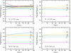 |
Fig. 1 Potential energies for O+H from the LCAO model for calculated symmetries and cores containing ionic crossings. The numbers on the right side of the plots indicate the asymptotic states as given in Table 2. |
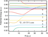 |
Fig. 2 Potential energies for O+H from the LCAO model, detailed view of 4Σ− with core |

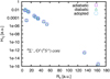 |
Fig. 3 Couplings H1j from the LCAO model plotted against the crossing distance Rc for 4Σ− with core |

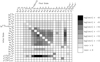 |
Fig. 4 Graphical representation of the rate coefficient matrix ⟨σv⟩ (in cm3 s−1) for inelastic O + H and O+ + H− collisions at temperature T = 6000 K. Results are from the LCAO asymptotic model. The logarithms in the legend are to base 10. |
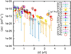 |
Fig. 5 Rate coefficients ⟨σv⟩ for O+H collision processes at 6000 K, plotted against the asymptotic energy difference between initial and final molecular states, ΔE. The data are shown for endothermic processes, i.e. excitation and ion-pair production. The initial states of the transition are colour-coded, and the processes leading to a final ionic state (ion-pair production) are circled. The points are from the LCAO model and the bars show the fluctuations. |
4 Concluding remarks
Excitation and charge transfer in low-energy O+H collisions has been studied using a method based on an asymptotic two-electron LCAO model of ionic-covalent interactions in the neutral atom-hydrogen-atom system, together with the multichannel Landau-Zener model (see B16). The method has been extended to include configurations involving excited states of hydrogen, namely the O (2p4.3P) + H(n = 2) configuration, but this extension was found to contribute only to processes with rather low rates when using an estimate for the two-electrontransition coupling proposed by Belyaev & Voronov (2017). Rate coefficients are presented for temperatures in the range 1000–20 000 K, and charge transfer and (de)excitation processes involving the first excited S-states, 4s.5 So and 4s.3 So, are found tohave the highest rates. The fluctuations calculated with alternate models are around an order of magnitude, which may give some indication of the uncertainty in these rates.
Since the O I triplet lines of interest in astrophysics correspond to 3s.5 So → 3p.5P, rates involving these states may be of importance. The work of Fabbian et al. (2009) shows the importance of the intersystem collisional coupling between the 3s.3So and 3s.5So states due to electron collisions, and Amarsi et al. (2016), when using the Drawin formula, has found the transition in the line due to hydrogen collisions to be of importance. The importance of these transitions seems to be borne out in preliminary statistical equilibrium calculations in stellar atmospheres (Amarsi, priv. comm.). Detailed testing of the sensitivity of the modelling to the data presented here will be carried out in the near future. The estimates calculated here for processes 3s.5 So → 3s.3So and 3s.5 So → 3p.5P give very low rate coefficients, ~4 × 10⁻¹⁴ cm3 s−1 and ~7 × 10⁻¹⁷ cm3 s−1, respectively.These low rates are uncertain since excitation processes involving these states are likely to have significant contributions from coupling mechanisms other than the ionic-covalent mechanism considered in the present model. It should be noted that if the de-excitation transition 3s.3 So → 3s.5So had a collisional coupling with similar efficiency to that for 2p4.1D → 2p4.3P from Krems et al. (2006), the excitation rate coefficient would be of the order of 10−13 to 10−12 cm3 s−1 (noting the much smaller energy separation). While there is no reason that the two transitions should behave in the same manner, this demonstrates the possibility for such couplings to provide significant contributions to the rate coefficients. The possible deficiencies of the Landau-Zener model for such short-range crossings at near-threshold energies should also be borne in mind (e.g. Belyaev et al. 1999; Barklem et al. 2011). Modern quantum chemistry calculations including potentials and couplings and detailed scattering calculations for the low-lying states of OH, at least up to states dissociating to O (3p) + H would be important to clarify this issue, and of potential importance in accurate modelling of the O I triplet in stellar spectra, and thus in obtaining accurate oxygen abundances in late-type stars including the Sun.
Acknowledgements
I thank Anish Amarsi for the comments on the draft, and for important preliminary feedback from astrophysical modelling. I also thank Thibaut Launoy for the useful discussions that illuminated issues regarding the angular momentum coupling factors. This work received financial support from the Swedish Research Council and the project grant “The New Milky Way” from the Knut and Alice Wallenberg Foundation.
References
- Adelman, S. A., & Herschbach, D. R. 1977, Mol. Phys., 33, 793 [NASA ADS] [CrossRef] [Google Scholar]
- Allende Prieto, C., Asplund, M., & Fabiani Bendicho, P. 2004, A&A, 423, 1109 [NASA ADS] [CrossRef] [EDP Sciences] [Google Scholar]
- Altrock, R. C. 1968, Sol. Phys., 5, 260 [NASA ADS] [CrossRef] [Google Scholar]
- Amarsi, A. M., Asplund, M., Collet, R., & Leenaarts, J. 2015, MNRAS, 454, L11 [NASA ADS] [CrossRef] [Google Scholar]
- Amarsi, A. M., Asplund, M., Collet, R., & Leenaarts, J. 2016, MNRAS, 455, 3735 [NASA ADS] [CrossRef] [Google Scholar]
- Anstee, S. D. 1992, Ph.D. Thesis, The University of Queensland, Australia [Google Scholar]
- Asplund,M. 2005, ARA&A, 43, 481 [NASA ADS] [CrossRef] [Google Scholar]
- Asplund, M., Grevesse, N., Sauval, A. J., Allende Prieto, C., & Kiselman, D. 2004, A&A, 417, 751 [NASA ADS] [CrossRef] [EDP Sciences] [Google Scholar]
- Bahcall, J. N., & Pinsonneault, M. H. 2004, Phys. Rev. Lett., 92, 121301 [NASA ADS] [CrossRef] [PubMed] [Google Scholar]
- Bahcall, J. N., Serenelli, A. M., & Basu, S. 2005, ApJ, 621, L85 [NASA ADS] [CrossRef] [Google Scholar]
- Bailey, J. E., Nagayama, T., Loisel, G. P., et al. 2015, Nature, 517, 56 [NASA ADS] [CrossRef] [Google Scholar]
- Barklem, P. S. 2007, A&A, 462, 781 [NASA ADS] [CrossRef] [EDP Sciences] [Google Scholar]
- Barklem, P. S. 2016a, A&ARv, 24, 1 [Google Scholar]
- Barklem, P. S. 2016b, Phys. Rev. A, 93, 042705 [NASA ADS] [CrossRef] [Google Scholar]
- Barklem, P. S. 2017, Phys. Rev. A, 95, 069906 [NASA ADS] [CrossRef] [Google Scholar]
- Barklem, P. S., Belyaev, A. K., & Asplund, M. 2003, A&A, 409, L1 [NASA ADS] [CrossRef] [EDP Sciences] [Google Scholar]
- Barklem, P. S., Belyaev, A. K., Guitou, M., et al. 2011, A&A, 530, A94 [NASA ADS] [CrossRef] [EDP Sciences] [Google Scholar]
- Barklem, P. S., Belyaev, A. K., Spielfiedel, A., Guitou, M., & Feautrier, N. 2012, A&A, 541, A80 [NASA ADS] [CrossRef] [EDP Sciences] [Google Scholar]
- Basu, S., & Antia, H. M. 2008, Phys. Rep., 457, 217 [NASA ADS] [CrossRef] [Google Scholar]
- Basu, S., Grevesse, N., Mathis, S., & Turck-Chièze, S. 2015, Space Sci. Rev., 196, 49 [NASA ADS] [CrossRef] [Google Scholar]
- Belyaev, A. K. 1993, Phys. Rev. A, 48, 4299 [NASA ADS] [CrossRef] [PubMed] [Google Scholar]
- Belyaev, A. K. 2013, Phys. Rev. A, 88, 052704 [NASA ADS] [CrossRef] [Google Scholar]
- Belyaev, A. K., & Barklem, P. S. 2003, Phys. Rev. A, 68, 062703 [NASA ADS] [CrossRef] [Google Scholar]
- Belyaev, A. K., & Voronov, Y. V. 2017, A&A, 606, A106 [NASA ADS] [CrossRef] [EDP Sciences] [Google Scholar]
- Belyaev, A. K., Grosser, J., Hahne, J., & Menzel,T. 1999, Phys. Rev. A, 60, 2151 [NASA ADS] [CrossRef] [MathSciNet] [Google Scholar]
- Belyaev, A. K., Barklem, P. S., Dickinson, A. S., & Gadéa, F. X. 2010, Phys. Rev. A, 81, 032706 [NASA ADS] [CrossRef] [Google Scholar]
- Belyaev, A. K., Barklem, P. S., Spielfiedel, A., et al. 2012, Phys. Rev. A, 85, 32704 [NASA ADS] [CrossRef] [Google Scholar]
- Belyaev, A. K., Yakovleva, S. A., & Barklem, P. S. 2014, A&A, 572, A103 [NASA ADS] [CrossRef] [EDP Sciences] [Google Scholar]
- Belyaev, A. K., Yakovleva, S. A., Guitou, M., et al. 2016, A&A, 587, A114 [NASA ADS] [CrossRef] [EDP Sciences] [Google Scholar]
- Chibisov, M., & Janev, R. 1988, Phys. Rep., 166, 1 [NASA ADS] [CrossRef] [Google Scholar]
- Delahaye, F., & Pinsonneault, M. H. 2006, ApJ, 649, 529 [NASA ADS] [CrossRef] [Google Scholar]
- Drawin, H. W. 1968, Z. Phys., 211, 404 [NASA ADS] [CrossRef] [EDP Sciences] [Google Scholar]
- Drawin, H. W. 1969, Z. Phys., 225, 483 [NASA ADS] [CrossRef] [EDP Sciences] [Google Scholar]
- Drawin, H. W., & Emard, F. 1973, Phys. Lett. A, 43, 333 [NASA ADS] [CrossRef] [Google Scholar]
- Easson, I., & Pryce, M. H. L. 1973, Can. J. Phys., 51, 518 [NASA ADS] [CrossRef] [Google Scholar]
- Eriksson, K., & Toft, S. C. 1979, A&A, 71, 178 [NASA ADS] [Google Scholar]
- Fabbian, D., Asplund, M., Barklem, P. S., Carlsson, M., & Kiselman, D. 2009, A&A, 500, 1221 [NASA ADS] [CrossRef] [EDP Sciences] [Google Scholar]
- Federman, S. R., & Shipsey, E. J. 1983, ApJ, 269, 791 [NASA ADS] [CrossRef] [Google Scholar]
- Fleck, I., Grosser, J., Schnecke, A., Steen, W., & Voigt, H. 1991, J. Phys. B: At. Mol. Opt. Phys., 24, 4017 [NASA ADS] [CrossRef] [MathSciNet] [Google Scholar]
- Grice, R., & Herschbach, D. R. 1974, Mol. Phys., 27, 159 [NASA ADS] [CrossRef] [Google Scholar]
- Guitou, M., Belyaev, A. K., Barklem, P. S., Spielfiedel, A., & Feautrier, N. 2011, J. Phys. B: At. Mol. Opt. Phys., 44, 035202 [NASA ADS] [CrossRef] [Google Scholar]
- Janev, R. K. 1976, J. Chem. Phys., 64, 1891 [NASA ADS] [CrossRef] [Google Scholar]
- Kiselman, D. 1993, A&A, 275, 269 [Google Scholar]
- Krems, R. V., Jamieson, M. J., & Dalgarno, A. 2006, ApJ, 647, 1531 [NASA ADS] [CrossRef] [Google Scholar]
- Lambert, D. L. 1993, Phys. Scr. T, 47, 186 [NASA ADS] [CrossRef] [Google Scholar]
- Langhoff, S. R., van Dishoeck, E. F., Wetmore, R., & Dalgarno, A. 1982, J. Chem. Phys., 77, 1379 [NASA ADS] [CrossRef] [Google Scholar]
- Lind, K., Asplund, M., Barklem, P. S., & Belyaev, A. K. 2011, A&A, 528, A103 [NASA ADS] [CrossRef] [EDP Sciences] [Google Scholar]
- Madhusudhan, N. 2012, ApJ, 758, 36 [NASA ADS] [CrossRef] [Google Scholar]
- Mendoza, C. 2017, ArXiv e-prints [arXiv:1704.03528] [Google Scholar]
- Nissen, P. E., Chen, Y. Q., Carigi, L., Schuster, W. J., & Zhao, G. 2014, A&A,568, A25 [NASA ADS] [CrossRef] [EDP Sciences] [Google Scholar]
- Olson, R. E., Smith, F. T., & Bauer, E. 1971, App. Opt., 10, 1848 [Google Scholar]
- Osorio, Y., Barklem, P. S., Lind, K., et al. 2015, A&A, 579, A53 [NASA ADS] [CrossRef] [EDP Sciences] [Google Scholar]
- Parlant, G., & Yarkony, D. R. 1999, J. Chem. Phys., 110, 363 [NASA ADS] [CrossRef] [Google Scholar]
- Pereira, T. M. D., Asplund, M., & Kiselman, D. 2009a, A&A, 508, 1403 [NASA ADS] [CrossRef] [EDP Sciences] [Google Scholar]
- Pereira, T. M. D., Kiselman, D., & Asplund, M. 2009b, A&A, 507, 417 [NASA ADS] [CrossRef] [EDP Sciences] [Google Scholar]
- Serenelli, A. M., Basu, S., Ferguson, J. W., & Asplund, M. 2009, ApJ, 705, L123 [NASA ADS] [CrossRef] [Google Scholar]
- Smirnov, B. M. 1965, Sov. Phys. Dok., 10, 218 [Google Scholar]
- Smirnov, B. M. 1967, Sov. Phys. Dok., 12, 242 [Google Scholar]
- Stasińska, G., Prantzos, N., Meynet, G., et al. 2012, EAS Pub. Ser., 54, Oxygen in the Universe (Les Ulis, France: EDP Sciences) [Google Scholar]
- Steenbock, W., & Holweger, H. 1984, A&A, 130, 319 [NASA ADS] [Google Scholar]
- Steffen, M., Prakapavičius, D., Caffau, E., et al. 2015, A&A, 583, A57 [NASA ADS] [CrossRef] [EDP Sciences] [Google Scholar]
- Tayal, S. S., & Zatsarinny, O. 2016, Phys. Rev. A, 94, 042707 [NASA ADS] [CrossRef] [Google Scholar]
- vanDishoeck, E. F., & Dalgarno, A. 1983, J. Chem. Phys., 79, 873 [NASA ADS] [CrossRef] [Google Scholar]
- Yarkony D. R. 1992, J. Chem. Phys., 97, 1838 [NASA ADS] [CrossRef] [Google Scholar]
- Zatsarinny, O., & Tayal, S. S. 2002, J. Phys. B: At. Mol. Opt. Phys., 35, 241 [NASA ADS] [CrossRef] [Google Scholar]
All Tables
Possible symmetries for O+H molecular states arising from various asymptotic atomic states, and the total statistical weights.
All Figures
|
Fig. 1 Potential energies for O+H from the LCAO model for calculated symmetries and cores containing ionic crossings. The numbers on the right side of the plots indicate the asymptotic states as given in Table 2. |
| In the text | |
|
Fig. 2 Potential energies for O+H from the LCAO model, detailed view of 4Σ− with core |
| In the text | |
|
Fig. 3 Couplings H1j from the LCAO model plotted against the crossing distance Rc for 4Σ− with core |
| In the text | |
|
Fig. 4 Graphical representation of the rate coefficient matrix ⟨σv⟩ (in cm3 s−1) for inelastic O + H and O+ + H− collisions at temperature T = 6000 K. Results are from the LCAO asymptotic model. The logarithms in the legend are to base 10. |
| In the text | |
|
Fig. 5 Rate coefficients ⟨σv⟩ for O+H collision processes at 6000 K, plotted against the asymptotic energy difference between initial and final molecular states, ΔE. The data are shown for endothermic processes, i.e. excitation and ion-pair production. The initial states of the transition are colour-coded, and the processes leading to a final ionic state (ion-pair production) are circled. The points are from the LCAO model and the bars show the fluctuations. |
| In the text | |
Current usage metrics show cumulative count of Article Views (full-text article views including HTML views, PDF and ePub downloads, according to the available data) and Abstracts Views on Vision4Press platform.
Data correspond to usage on the plateform after 2015. The current usage metrics is available 48-96 hours after online publication and is updated daily on week days.
Initial download of the metrics may take a while.