| Issue |
A&A
Volume 610, February 2018
|
|
|---|---|---|
| Article Number | A36 | |
| Number of page(s) | 6 | |
| Section | Celestial mechanics and astrometry | |
| DOI | https://doi.org/10.1051/0004-6361/201731901 | |
| Published online | 21 February 2018 | |
Measurement of the solar system acceleration using the Earth scale factor
1
Geoscience Australia,
PO Box 378,
Canberra
2601, Australia
e-mail: Oleg.Titov@ga.gov.au
2
Technische Universität Wien, Department of Geodesy and Geoinformation,
Gusshausstrasse 27-29,
1040
Vienna, Austria
Received:
6
September
2017
Accepted:
30
November
2017
Aim. We propose an alternative method to detect the secular aberration drift induced by the solar system acceleration due to the attraction to the Galaxy centre. This method is free of the individual radio source proper motion caused by intrinsic structure variation.
Methods. We developed a procedure to estimate the scale factor directly from very long baseline interferometry (VLBI) data analysis in a source-wise mode within a global solution. The scale factor is estimated for each reference radio source individually as a function of astrometric coordinates (right ascension and declination). This approach splits the systematic dipole effect and uncorrelated motions on the level of observational parameters.
Results. We processed VLBI observations from 1979.7 to 2016.5 to obtain the scale factor estimates for more than 4000 reference radio sources. We show that the estimates highlight a dipole systematics aligned with the direction to the centre of the Galaxy. With this method we obtained a Galactocentric acceleration vector with an amplitude of 5.2 ± 0.2 μas/yr and direction αG = 281∘± 3∘ and δG = −35∘± 3∘.
Key words: astrometry / reference systems / techniques: interferometric
© ESO 2018
 Open Access article, published by EDP Sciences, under the terms of the Creative Commons Attribution License (http://creativecommons.org/licenses/by/4.0), which permits unrestricted use, distribution, and reproduction in any medium, provided the original work is properly cited.
1 Introduction
The solar system is rotating around the Galactic centre with a period of approximately 200 million years. The solar system barycentre shows, therefore, rotational acceleration in the direction of the Galactic centre of 5–6 microarcseconds of arc per year (μas/yr) and this effect, the secular aberration drift (SAD), results in a systematic proper motion of reference radio sources around the sky.
The theoretical prediction of the dipole systematics (Fanselow 1983; Bastian 1995; Eubanks et al. 1995; Gwinn et al. 1997; Sovers et al. 1998; Mignard 2002; Kovalevsky 2003; Kopeikin & Makarov 2006) was recently confirmed after the analysis of a global set of very long baseline interferometry (VLBI) data since 1979 (Titov 2011; Xu et al. 2012, 2013; Titov & Lambert 2013, 2016; MacMillan 2014). The magnitude of the dipole systematics is consistent, whereas the estimate of the dipole direction varies mostly owing to the strong influence of the variability of the relativistic jets (Table 1). The individual apparent proper motion of the reference radio sources may reach 0.5 ms of arc/yr (i.e. 100 times of the dipole effect). Therefore, the exclusion of astrometrically unstable radio sources from the analysis is a highly labour-intensive process that yields marginal results with a formal error of 1 μas/yr (e.g. Titov & Lambert 2013). In the meantime, Mignard & Klioner (2012) showed that the Gaia mission will obtain the parameters of the Galactocentric acceleration with a formal error of 0.2 μas/yr, i.e. five times better. Therefore, we are seeking methods to improve the VLBI data results.
Theoretically, the Galactocentric acceleration vector points to the centre of the Galaxy, which is supposed to be the location of the compact radio source Sagittarius A* with the estimated coordinates αG = 267∘ for right ascension and δG = −29∘ for declination having the absolute position error of 0. ′′12 (Reid & Brunthaler 2004). A comprehensive instruction to calculate the acceleration amplitude using the International Astronomical Union-recommended Galactic centre distance (Rgal = 8.5 kpc) with the Galaxy rotation velocity at Rgal (Vgal = 220 km s−1) and assuming the circular type of motion is given, for examplein Kovalevsky (2003) or Titov (2011). This results in a value  , which can be converted to the acceleration vector a with the magnitude of 3.8 μas/yr. There are dozens of papers devoted to revision of the parameters Rgal and Vgal based on different modern observation data and analysis strategies. For instance, Reid et al. (2009) provided new meanings for Rgal = 8.4 ± 0.6 kpc and Vgal = 254 ± 16 km s−1. The corresponding acceleration amplitude is 2.49 × 10⁻¹³ km s−2 and the amplitude A of the dipole proper motion equals to 5.1 μas/yr. In one of the most recent publications, de Grijs & Bono (2016) recommended a downward adjustment of the Rgal to 8.3 kpc and an upward revision of Vgal in the range from 232 km s−1 to 266 km s−1. The corresponding amplitude of the Galactocentric acceleration vector lies therefore within the range (2.10 ÷ 2.76) × 10−13 km s−2 followed by the expected amplitude of the dipole proper motion between 4.3 and 5.7 μas/yr.
Titov (2011) noted that the conventional equation of the geodetic VLBI group delay (Petit & Luzum 2010, chap. 11) could be altered to accommodate the Galactocentric acceleration. This modification provides a way to estimate the SAD either as a dipole systematics in proper motions or as a systematic effect in the VLBI scale. Section 2 recalls the corresponding mathematical equations and demonstrates the advantage of the latter option. In Sect. 3, we present the results obtained by applying the new method to analysis of VLBI data during 1979.7–2016.5 together with the SAD estimates from global VLBI adjustments.
Estimates of the SAD parameters from available publicationsif only a dipole component is estimated.
2 Basic equations
The fundamental geodetic VLBI observable, the group delay τgroup, is the first derivative of the phase with respect to angular frequency ofthe incoming signal. A group of eight channels within the frequency band from 8.1 to 8.9 GHz (known as X -band) measures the phases simultaneously to obtain the group delay by the least-squares adjustment. The conventional group delay model approximating the observed VLBI data is given by Petit & Luzum (2010, Chap. 11) as
 (1)
where b is the vector of baseline b = r2 − r1, s is the barycentric (solar system barycentre) unit vector of radio source, V⊕ is the barycentric velocity of the geocentre, w2 is the geocentric velocity of the second station, c is the speed of light, G is the gravitational constant, M⊙ is the mass of the Sun, and R⊕⊙ is the geocentric distance to the Sun.
(1)
where b is the vector of baseline b = r2 − r1, s is the barycentric (solar system barycentre) unit vector of radio source, V⊕ is the barycentric velocity of the geocentre, w2 is the geocentric velocity of the second station, c is the speed of light, G is the gravitational constant, M⊙ is the mass of the Sun, and R⊕⊙ is the geocentric distance to the Sun.
The term  is related to the general relativity effect. The impact of w2 is small and may be ignored for sake of simplicity. After these alterations Eq. (1) is given by
 (2)
(2)
Equation (2) now comprises only the effects of special relativity of orders  and
and  . Leaving only the terms of
  and using the Taylor series expansion for
  , Eq. (2) comes down to the main aberration effect
 (3)
where the second term represents the correction for the annual aberration
(3)
where the second term represents the correction for the annual aberration
 (4)
(4)
Titov (2011) showed that the Galactocentric acceleration vector a can be added to the conventional Eq. (1) by replacing the barycentric velocity V⊕ with the sum V⊕ + aΔt, where Δt is the time since the reference epoch 2000.0. As a result the corresponding correction for the aberration effect is
 (5)
(5)
Since the proper motions affect the source positions in the form s′ = s + Δs = s + μΔt, the vector of proper motion should be represented as a sum of two components μ = μ1 + μ2 = s(s⋅μ) + μ2, where μ2 is the component along the acceleration vector a, and μ1 has the direction perpendicular to vectors a and s . Then, the additional delay induced by random-like apparent proper motion of a radio source is given by
 (6)
(6)
It should be noted that even if the projection of Δs from Eq. (4) on the vector s is zero, i.e. s ⋅ Δ s = 0, the time delay in Eqs. (5) and (6) describes a projection of Δ s on the baseline vector b. Therefore, in a general case, the delays in Eqs. (5) and (6) as well as both components of Eq. (5),  and
and  , are non-zero values.
From the sum of Eqs. (5) and (6),
 (7)
it can be concluded that the first term, proportional to the geometric delay
(7)
it can be concluded that the first term, proportional to the geometric delay  , is sensitive to the component μ1 alone. This implies that the estimate of the Galactocentric acceleration with the first term of Eq. (7) is likely to be more accurate than from analysis of individual proper motion of reference radio sources.
If the model (Eq. (1)) described the observations perfectly, then the scale factor (F) determined by
 (8)
is equal to unity for all observations, i.e. F ≡ 1 (e.g. MacMillan 2017). However, if the proper motions are not estimated, then the first term in Eq. (7) as a part of the group delay (Eq. (1)) is considered as a contribution to the scale factor. After division in Eq. (8), the scale factor is given by
(8)
is equal to unity for all observations, i.e. F ≡ 1 (e.g. MacMillan 2017). However, if the proper motions are not estimated, then the first term in Eq. (7) as a part of the group delay (Eq. (1)) is considered as a contribution to the scale factor. After division in Eq. (8), the scale factor is given by
 (9)and manifests itself as a variable parameter depending on the Galactocentric acceleration, radio source position, and the time since a reference epoch. Consequently, the partial derivative of the group delay w.r.t. the scale factor as a time-dependent effect is given by
 (10)or it can be expressed as a time-independent effect in the following way:
 (11)
(11)
3 Analysis of VLBI data
In this paper we analyse almost all VLBI sessions provided by the International VLBI Service for Geodesy and Astrometry (IVS; Schuh & Behrend 2012) together with the Very Long Baseline Array (VLBA) Calibrator Survey (VCS) observing sessions VCS1-6 (Beasley et al. 2002; Fomalont et al. 2003; Petrov et al. 2005, 2006, 2008; Kovalev et al. 2007)and VCS-II (Gordon et al. 2016), i.e. 5825 observing sessions from 1979.7 until 2016.5. A dedicated observational project was started in Australia with Parkes 64 metre radio telescope and other Long Baseline Array (LBA) facilities since 2004 to enforce astrometry in the southern hemisphere.
The VLBI analysis was carried out with the software VieVS (Böhm et al. 2012) and processing of our standard reference solution (P1) followed the International Earth Rotation and Reference Systems Service (IERS) Conventions 2010 (Petit & Luzum 2010) and the technique specific VLBI analysis recommendations. Further details of the parametrisation and analysis set-up for our standard VLBI solution are given in Krásná et al. (2015).
3.1 Scalefactor
The scale factor is usually not estimated in the routine procedure ofgeodetic VLBI data analysis. However, there is a possibility to estimate the scale factor either as a single parameter (in a session-wise or global adjustment) or as a specific parameter for each radio source individually within the global solution, similar to the radio source coordinates.
3.1.1 Scale factor as a single parameter
Using Eq. (10) we obtained the session-wise estimates of the scale factor from the standard solution (Fig. 1), where the station positions and velocities were fixed to the a priori values in ITRF2014 (Altamimi et al. 2016). The Earth orientation parameters and positions of the radio sources (no-net-rotation on the defining ICRF2 radio sources; Fey et al. 2009, 2015) were estimated in the usual way on a session-wise basis. The green line in the figure shows the smoothed estimates using the local least-squares regression. The annual periodicity visible in the scale factor estimates is predominantly due to the omitted hydrology loading corrections in the station coordinates, as shown by MacMillan (2017), and the weighted mean over the estimated scale corrections of 0.7 part-per-billion (ppb) is in accordance with the definition of the ITRF2014 scale, which is obtained by the arithmetic average of the scale of satellite laser ranging (SLR) and VLBI solutions. The scale discrepancy between these two combined solutions building the ITRF2014 is 1.37 ± 0.10 ppb at epoch 2010.0 (Altamimi et al. 2016). There is an ongoing discussion about the reason for the systematic difference in scale as determined from the two high accurate space geodetic techniques. Recently, Appleby et al. (2016) pointed out that there seems to be a range bias in the case of SLR, which would be responsible for about the half of the obtained scale discrepancy.
Figure 2 shows the respective formal errors of the scale factor estimates presented in Fig. 1. A rapid decrease of the formal errors can be seen between the early VLBI years and 1995. The most accurate estimates of the scale factor belong to the RDV (Research and Development VLBA) sessions and these are highlighted with the magenta dots.
 |
Fig. 1 Session-wise corrections to the scale factor Δ F w.r.t. ITRF2014. The green line follows the smoothed estimates using the local least-squares regression. The magenta dots highlight the estimates from RDV sessions. |
 |
Fig. 2 Formal errors of the session-wise corrections to the scale factor Δ F w.r.t. ITRF2014. The magenta dots highlight the formal errors from RDV sessions, shown in detail in the lower plot. |
3.1.2 Scale factor as a specific global parameter for each radio source
In this section we focus on the globally computed scale factor correction, that is from a common adjustment of the VLBI sessions, where we estimated this correction as a specific parameter for each radio source individually (except the 39 special handling sources). We ran a global solution with a standard parametrisation (P1), where corrections to the terrestrial reference frame (i.e. position and linear velocity of VLBI radio telescopes), celestial reference frame (i.e. position of radio sources), and the individual scale factor for each radio source are determined. Using Eq. (10) for the partial derivative we obtained the scale factor corrections plotted in the upper part of Fig. 3 as a function of right ascension (left-hand side) and as a function of declination (right-hand side). As a next step, the conventional equation for the group delay model (Petit & Luzum 2010, Chap. 11) is extended by the Galactocentric acceleration vector a following Titov (2011). The SAD effect is reduced from the measurements a priori using the following values: A = 5μas/yr, αG = 267∘ and δG = −29∘. We refer to this parametrisation as to P2. Applying the P2 we ran asecond global solution. The difference in Δ F (lower part of Fig. 3) between the standard solution and the solution with reduced SAD effect shows a clear systematic effect arising from the omitted SAD effect in the standard parametrisation. The maximum difference in the right ascension (left-hand side) and declination (right-hand side) coincides consequently with the direction to the Galactic centre and reaches about 0.2 ppb, whereas the weighted mean of the difference is −0.016 ppb.
To dispose of the time dependency of the scale factor we express the partial derivative of the group delay with Eq. (11). Another two global solutions (with P1 and P2 parametrisation) were computed. The resulting annual drift of the scale factor corrections Δ F∕Δt from P1 is plotted as a function of equatorial coordinates in the upper part of Fig. 4 and the lower part shows the difference between the P1 and P2 parametrisation. Comparing the Figs. 3 and 4 it is obvious that the scale factor corrections, expressed as a time-independent effect in the [ppb/yr] units, are free of large outliers. The annual variation of the scale factor due to the omitted SAD effect reaches about 0.02 ppb/yr, which reflects the mean observing time of about 10 yr over all included radio sources.
Since we estimated the source-wise scale corrections together with the terrestrial (TRF) and celestial (CRF) reference frame within the global adjustment, a constant bias in the scale difference propagates also to the estimated terrestrial reference frame. Comparison of the TRF from the parametrisation P1 minus TRF from P2 in terms of the 14-parameters weighted Helmert transformation gives a negligible difference of −0.011 ± 0.001 ppb (−0.07 ± 0.01 mm) for the scale. It means that omitting the Galactocentric acceleration effect in the VLBI analysis does not have any significant effect on the global scale of the estimated TRF.
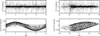 |
Fig. 4 Annual drift of the scale factor corrections Δ F∕Δ t for all 4097 radio sources as a function of equatorial coordinatesw.r.t. right ascension (left-hand side) and declination (right-hand side). Upper plots: estimates from the parametrisation P1; lower plots: difference P1 minus P2. |
 |
Fig. 3 Correction to the scale factor Δ F for all 4097 radio sources as a function of equatorial coordinatesw.r.t. right ascension (left-hand side) and declination (right-hand side). Upper plots: estimates from the parametrisation P1; lower plots: difference P1 minus P2. |
3.2 Galactocentric acceleration vector
3.2.1 Galactocentric acceleration vector from source-wise scale factor
The individual scale factor corrections ΔF∕Δt could be fitted by the following model:
 (12)
using the components of the acceleration vector a1, a2, a3
(12)
using the components of the acceleration vector a1, a2, a3
 (13)where A is the amplitude of the Galactocentric acceleration and αG, δG are the equatorial coordinates of the vector direction. The three parameters determining the dipole (a1, a2, a3) are to be estimated using the standard least-squares method. Then the amplitude A and the coordinates αG, δG are given by
 (14)
(14)
 (15)
(15)
Table 2 shows the estimated dipole components from fitting the annual variation of the scale factor for different cut-off limits for the number of observations N of each radio source in order to mitigate the effect of rarely observed radio sources and to verify the stability of the solution with respect to N. For a wide range of N (from 50 to 20 000), where the compromise between the number of observations and the number of sources is fulfilled, the amplitude of the dipole effect varies between 4.8 and 5.3 μas/yr, and the best formal error is 0.2 μas/yr, i.e. much less than from the analysis of proper motions (Titov 2011; Titov & Lambert 2013, 2016). One can conclude that this approach is less sensitive to the peculiar behaviour of the active galactic nuclei. The estimated direction in declination (from −28∘ to −35∘) gets close to the value estimated by Reid & Brunthaler (2004) within its formal error, whereas there is a offset of 14∘ between the estimated direction in right ascension ( ~281∘) and the value 267∘ reported by Reid & Brunthaler (2004). The bias can be explained by the apparent proper motion of astrometrically unstable radio sources. This instability is caused by internal motion of matter in relativistic jet.
As shown in Fig. 1 the time series of the scale factor estimates contains an annual signal originating predominantly from the omitted hydrology loading corrections. Therefore, we computed another solution based on P1, where we applied the hydrology loading displacement time series provided by the NASA Goddard Space Flight Center VLBI group (Eriksson & MacMillan 2014) on the station coordinates a priori. We ran again a global solution where the annual drift of the individual scale factor corrections was estimated in the same way as in the solutions mentioned above. From fitting the estimates belonging to radio sources with more than 50 observations, the following dipole components were obtained: A = 5.1 ± 0.2μas/yr, αG = 279∘± 3∘ and δG = −35∘± 3∘. This yields a difference of 0.1 μas/yr in A and 2∘ in αG with respect to the solution based on parametrisation P1, which lies within the formal errors of the estimates and shows that the seasonal hydrology variation in the station coordinates does not have any significant effect on the estimated dipole components.
Estimates and their formal errors of the dipole components in the Δ F∕Δ t a posteriori from the parametrisation P1.
3.2.2 Galactocentric acceleration vector as a global parameter
The dipole components can be also estimated as global parameters in a VLBI solution in the form of the Galactocentric acceleration vector. The parametrisation P2 allowed us to build the partial derivative of the group delay with respect to the three components (a1, a2, a3) of a. We ran a global solution in which corrections to the terrestrial reference frame (i.e. position and linear velocity of VLBI radio telescopes), celestial reference frame (i.e. position of radio sources), and the three components of the Galactocentric acceleration vector were determined. Table 3 summarises the estimated SAD parameters given with the amplitude A of the Galactocentric acceleration vector and with the direction in αG and δG. The first column shows the resulting Galactocentric acceleration vector from a global adjustment of all VLBI sessions in our dataset (i.e. from 1979.7 until 2016.5). The second column contains the Galactocentric acceleration vector determined within an adjustment of large global networks only, represented by the following specific IVS programmes: the National Earth Orientation Service (NEOS-A) sessions, Rapid turnaround IVS-R1 and IVS-R4 sessions, and all available two-weeks CONTinuous campaigns (CONT), i.e. ~2000 sessions from 1993 until 2016.5. Both solutions yield a value for the amplitude A, which is consistent with the estimates published in the last few years (Titov 2011; Xu et al. 2012, 2013; Titov & Lambert 2013, 2016; MacMillan 2014). The direction in declination of the vector coincides with the value estimated by Reid & Brunthaler (2004) if only the large network sessions were included in the solution, which implies that this procedure is sensitive to the inclusion of weak networks.
Galactocentric acceleration vector estimated as global parameter within VLBI solutions.
4 Conclusions
We introduce a new method to detect the SAD induced by the Galactocentric acceleration from the geodetic VLBI measurements. It is based on fitting the scale factor corrections estimated for each source individually within a global solution. In Titov & Lambert (2013) we used the individual proper motion of reference radio sources to visualise the dipole effect caused by the Galactocentric acceleration. However, because of contamination by large apparent motions induced by relativistic jet, the proper motions have large random noise almosthiding the dipole systematics. However, if the dipole components in proper motion are not estimated, the systematic effect comes to the scale effect that, in contrast to the proper motion, is free of the relativistic jet problems.
From fitting the individual scale factor corrections of sources with more than 50 observations during 1979.7–2016.5 we obtained a Galactocentric acceleration vector with an amplitude of 5.2 ± 0.2 μas/yr and direction αG = 281∘± 3∘ and δG = −35∘± 3∘. The SAD was also estimated directly within a global adjustment of the VLBIdata. The Galactocentric acceleration vector determined from the selected large network IVS sessions after 1993 (A = 5.4 ± 0.4μas/yr, αG = 273∘± 4∘, δG = −27∘± 8∘) is closer to the value reported by recent papers (e.g. Reid & Brunthaler 2004; de Grijs & Bono 2016) than the estimate from the entire VLBI history. The formal error of the amplitude of the acceleration vector estimated by means of the scale factor is about five times better than the estimate from the proper motions (Titov & Lambert 2016) and comparable to the accuracy expected to be obtained with the Gaia mission (Mignard & Klioner 2012). This demonstrates the advantage of the new approach with respect to the traditional procedure.
Our result also points out the potential impact of neglecting the Galactocentric acceleration on the scale factor and, finally, on the geodetic positions of the radio telescopes. The scale factor becomes dependent on the positions of the reference radio sources, i.e. larger in the direction of the Galactic anti-centre, and smaller in the direction of the Galactic centre. In a global sense, the quality of the geodetic results is worsening and, moreover, the loss of quality would increase linearly with time.
The results presented in this paper were computed with the VieVS software and verified with the OCCAM software package.
Acknowledgments
The authors thank the anonymous referee for her/his constructive comments. The authors acknowledge the IVS and all its components for providing VLBI data (Nothnagel et al. 2015). The Long Baseline Array is part of the Australia Telescope National Facility which is funded by the Australian Government for operation as a National Facility managed by CSIRO (P483 and V515). This study also made use of data collected through the AuScope initiative. AuScope Ltd is funded under the National Collaborative Research Infrastructure Strategy (NCRIS), an Australian Commonwealth Government Programme. The Very Long Baseline Array (VLBA) is operated by the National Radio Astronomy Observatory, which is a facility of the National Science Foundation, and operated under cooperative agreement by Associated Universities, Inc. Hana Krásná works within the Hertha Firnberg position T697-N29, funded by the Austrian Science Fund (FWF). This paper has been published with the permission of the Geoscience Australia CEO.
References
- Altamimi, Z., Rebischung, P., Métivier, L., & Collilieux, X. 2016, J. Geophys. Res. Solid Earth, 121, 6109 [Google Scholar]
- Appleby, G., Rodríguez, J., & Altamimi, Z. 2016, J. Geodesy, 90, 1371 [NASA ADS] [CrossRef] [Google Scholar]
- Bastian, U. 1995, in Proc. RGO-ESA Workshop on Future Possibilities for Astrometry in Space, ESA SP-379, eds. M. A. C. Perryman & F. Van Leeuwen, 99 [Google Scholar]
- Beasley, A. J., Gordon, D., Peck, A. B., et al. 2002, ApJS, 141, 13 [NASA ADS] [CrossRef] [Google Scholar]
- Böhm, J., Böhm, S., Nilsson, T., et al. 2012, in IAG Symposium 2009, eds. S. Kenyon, M. Pacino, & U. Marti, 136, 1007 [Google Scholar]
- de Grijs, R., & Bono, G. 2016, ApJS, 227, 5 [NASA ADS] [CrossRef] [Google Scholar]
- Eriksson, D., & MacMillan, D. S. 2014, J. Geodesy, 88, 675 [NASA ADS] [CrossRef] [Google Scholar]
- Eubanks, T. M., Matsakis, D. N., Josties, F. J., et al. 1995, in International Astronomical Union (IAU) Symp., eds. E. Hog & P. K. Seidelmann, 166, 283 [NASA ADS] [Google Scholar]
- Fanselow, J. L. 1983, Observation Model and Parameter Partials for the JPL VLBI Parameter Estimation Software MASTERFIT-V1.0 (JPL Publication 83-39) [Google Scholar]
- Fey, A., Gordon, D., & Jacobs, C. S. 2009, The Second Realization of the International Celestial Reference Frame by Very Long Baseline Interferometry, (IERS Technical Note No. 35) [Google Scholar]
- Fey, A., Gordon, D., Jacobs, C. S., et al. 2015, AJ, 150, 58 [NASA ADS] [CrossRef] [Google Scholar]
- Fomalont, E. B., Petrov, L., MacMillan, D. S., Gordon, D., & Ma, C. 2003, AJ, 126, 2562 [NASA ADS] [CrossRef] [Google Scholar]
- Gordon, D., Jacobs, C., Beasley, A., et al. 2016, AJ, 151, 154 [NASA ADS] [CrossRef] [Google Scholar]
- Gwinn, C. R., Eubanks, T. M., Pyne, T., Birkinshaw, M., & Matsakis, D. N. 1997, ApJ, 485, 87 [NASA ADS] [CrossRef] [Google Scholar]
- Kopeikin, S. M., & Makarov, V. V. 2006, AJ, 131, 1471 [NASA ADS] [CrossRef] [Google Scholar]
- Kovalev, Y. Y., Petrov, L., Fomalont, E., & Gordon, D. 2007, AJ, 133, 1236 [NASA ADS] [CrossRef] [Google Scholar]
- Kovalevsky, J. 2003, A&A, 404, 743 [NASA ADS] [CrossRef] [EDP Sciences] [Google Scholar]
- Krásná, H., Malkin, Z., & Böhm, J. 2015, J. Geodesy, 89, 1019 [NASA ADS] [CrossRef] [Google Scholar]
- MacMillan, D. S. 2014, AGU Fall Meeting Abstracts [Google Scholar]
- MacMillan, D. S. 2017, J. Geodesy, 91, 819 [NASA ADS] [CrossRef] [Google Scholar]
- Mignard, F. 2002, in GAIA: A European Space Project, eds. O. Bienaymé & C. Turon, EAS Publication Series, 2, 327 [Google Scholar]
- Mignard, F., & Klioner, S. 2012, A&A, 547, A59 [NASA ADS] [CrossRef] [EDP Sciences] [Google Scholar]
- Nothnagel, A., Alef, W., Amagai, J., et al. 2015, GFZ Data Services (Potsdam, Germany: Helmoltz Centre) [Google Scholar]
- Petit, G., & Luzum, B. 2010, IERS Conventions 2010 (IERS Technical Note No. 36) [Google Scholar]
- Petrov, L., Kovalev, Y. Y., Fomalont, E., & Gordon, D. 2005, AJ, 129, 1163 [NASA ADS] [CrossRef] [Google Scholar]
- Petrov, L., Kovalev, Y. Y., Fomalont, E., & Gordon, D. 2006, AJ, 131, 1872 [NASA ADS] [CrossRef] [Google Scholar]
- Petrov, L., Kovalev, Y. Y., Fomalont, E., & Gordon, D. 2008, AJ, 136, 580 [NASA ADS] [CrossRef] [Google Scholar]
- Reid, M. J., & Brunthaler, A. 2004, ApJ, 616, 872 [NASA ADS] [CrossRef] [Google Scholar]
- Reid, M. J., Menten, K. M., Zheng, X. W., et al. 2009, ApJ, 700, 137 [NASA ADS] [CrossRef] [Google Scholar]
- Schuh, H., & Behrend, D. 2012, J. Geodyn., 61, 68 [NASA ADS] [CrossRef] [Google Scholar]
- Sovers, O. J., Fanselow, J. L., & Jacobs, C. S. 1998, Rev. Mod. Phys., 70, 1393 [NASA ADS] [CrossRef] [Google Scholar]
- Titov, O. 2011, Astron. Rep., 55, 91 [NASA ADS] [CrossRef] [Google Scholar]
- Titov, O., & Lambert, S. 2013, A&A, 559, A95 [NASA ADS] [CrossRef] [EDP Sciences] [Google Scholar]
- Titov, O., & Lambert, S. 2016, ArXiv e-prints [arXiv:1603.09416] [Google Scholar]
- Xu, M. H., Wang, G. L., & Zhao, M. 2012, A&A, 544, A135 [NASA ADS] [CrossRef] [EDP Sciences] [Google Scholar]
- Xu, M. H., Wang, G. L., & Zhao, M. 2013, MNRAS, 430, 2633 [NASA ADS] [CrossRef] [Google Scholar]
All Tables
Estimates of the SAD parameters from available publicationsif only a dipole component is estimated.
Estimates and their formal errors of the dipole components in the Δ F∕Δ t a posteriori from the parametrisation P1.
Galactocentric acceleration vector estimated as global parameter within VLBI solutions.
All Figures
|
Fig. 1 Session-wise corrections to the scale factor Δ F w.r.t. ITRF2014. The green line follows the smoothed estimates using the local least-squares regression. The magenta dots highlight the estimates from RDV sessions. |
| In the text | |
|
Fig. 2 Formal errors of the session-wise corrections to the scale factor Δ F w.r.t. ITRF2014. The magenta dots highlight the formal errors from RDV sessions, shown in detail in the lower plot. |
| In the text | |
|
Fig. 4 Annual drift of the scale factor corrections Δ F∕Δ t for all 4097 radio sources as a function of equatorial coordinatesw.r.t. right ascension (left-hand side) and declination (right-hand side). Upper plots: estimates from the parametrisation P1; lower plots: difference P1 minus P2. |
| In the text | |
|
Fig. 3 Correction to the scale factor Δ F for all 4097 radio sources as a function of equatorial coordinatesw.r.t. right ascension (left-hand side) and declination (right-hand side). Upper plots: estimates from the parametrisation P1; lower plots: difference P1 minus P2. |
| In the text | |
Current usage metrics show cumulative count of Article Views (full-text article views including HTML views, PDF and ePub downloads, according to the available data) and Abstracts Views on Vision4Press platform.
Data correspond to usage on the plateform after 2015. The current usage metrics is available 48-96 hours after online publication and is updated daily on week days.
Initial download of the metrics may take a while.