| Issue |
A&A
Volume 610, February 2018
|
|
|---|---|---|
| Article Number | A46 | |
| Number of page(s) | 10 | |
| Section | Stellar structure and evolution | |
| DOI | https://doi.org/10.1051/0004-6361/201730769 | |
| Published online | 23 February 2018 | |
A universal relation for the propeller mechanisms in magnetic rotating stars at different scales
1
INAF – Osservatorio Astronomico di Brera,
Via E. Bianchi 46,
23807
Merate,
LC, Italy
e-mail: This email address is being protected from spambots. You need JavaScript enabled to view it.
2
INAF – Osservatorio Astronomico di Roma,
Via Frascati 33,
00078
Monteporzio Catone,
Roma, Italy
3
INAF – Istituto di Astrofisica Spaziale e Fisica Cosmica – Milano,
Via E. Bassini 15,
20133
Milano, Italy
4
INAF – Osservatorio Astronomico di Capodimonte,
Salita Moiariello 16,
80131
Napoli, Italy
Received:
11
March
2017
Accepted:
13
November
2017
Abstract
Accretion of matter onto a magnetic, rotating object can be strongly affected by the interaction with its magnetic field. This occurs in a variety of astrophysical settings involving young stellar objects, white dwarfs, and neutron stars. As matter is endowed with angular momentum, its inflow toward the star is often mediated by an accretion disc. The pressure of matter and that originating from the stellar magnetic field balance at the magnetospheric radius: at smaller distances the motion of matter is dominated by the magnetic field, and funnelling towards the magnetic poles ensues. However, if the star, and thus its magnetosphere, is fast spinning, most of the inflowing matter will be halted at the magnetospheric radius by centrifugal forces, resulting in a characteristic reduction of the accretion luminosity. The onset of this mechanism, called the propeller, has been widely adopted to interpret a distinctive knee in the decaying phase of the light curve of several transiently accreting X-ray pulsar systems. By comparing the observed luminosity at the knee for different classes of objects with the value predicted by accretion theory on the basis of the independently measured magnetic field, spin period, mass, and radius of the star, we disclose here a general relation for the onset of the propeller which spans about eight orders of magnitude in spin period and ten in magnetic moment. The parameter-dependence and normalisation constant that we determine are in agreement with basic accretion theory.
Key words: stars: neutron / X-rays: binaries / accretion, accretion discs / magnetic fields
© ESO 2018
1 Introduction
The innermost regions of accretion flows towards a magnetic star are governed by the magnetic field which channels the inflowing material onto the magnetic polar caps. The motion of the inflowing matter starts being dominated by the magnetic field at the magnetospheric radius, where the star’s magnetic field pressure balances the ram pressure of the infalling matter. In spherical symmetry, simple theory predicts that this will occur at the Alfvén radius,
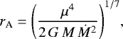 (1)
where μ is the magnetic dipole moment (μ = B R3), Ṁ is the mass accretion rate, G is the gravitational constant, and M, R, and B are the star mass, radius, and dipolar magnetic field, respectively (Pringle & Rees 1972; Frank et al. 2002). In interacting binaries, the accreting matter is endowed with a large angular momentum, which leads to the formation of an accretion disc where matter spirals in by transferring angular momentum outwards, while gravitational energy is converted into internal energy and/or radiation. The interaction of an accretion disc with a magnetosphere has been investigated extensively through theoretical studies (Ghosh & Lamb 1979; Wang 1987; Shu et al. 1994; Lovelace et al. 1995; Li & Wickramasinghe 1997; D’Angelo & Spruit 2012; Parfrey et al. 2016) and through magnetohydrodynamical simulations (Romanova et al. 2003; Zanni & Ferreira 2013).
(1)
where μ is the magnetic dipole moment (μ = B R3), Ṁ is the mass accretion rate, G is the gravitational constant, and M, R, and B are the star mass, radius, and dipolar magnetic field, respectively (Pringle & Rees 1972; Frank et al. 2002). In interacting binaries, the accreting matter is endowed with a large angular momentum, which leads to the formation of an accretion disc where matter spirals in by transferring angular momentum outwards, while gravitational energy is converted into internal energy and/or radiation. The interaction of an accretion disc with a magnetosphere has been investigated extensively through theoretical studies (Ghosh & Lamb 1979; Wang 1987; Shu et al. 1994; Lovelace et al. 1995; Li & Wickramasinghe 1997; D’Angelo & Spruit 2012; Parfrey et al. 2016) and through magnetohydrodynamical simulations (Romanova et al. 2003; Zanni & Ferreira 2013).
In somemodels (Ghosh & Lamb 1979; Shu et al. 1994; Wang 1987) the boundary between the disc and the magnetosphere is expressed through a slight modification of Eq. (1): the dependence on the parameters remains the same, but the magnetospheric radius is rm = ξ rA, with ξ ~0.1–1 a normalisation factor that depends on the assumptions of different theories (Ghosh & Lamb 1979; Spruit & Taam 1993; Wang 1987; Kluźniak & Rappaport 2007). Models which consider different types of disc magnetic-field threading and outflow-launching mechanisms also lead to a similar dependence on the parameters (Shu et al. 1994; Lovelace et al. 1995; Li & Wickramasinghe 1997). Other studies predict instead a different dependence of the magnetospheric radius on the stellar parameters. For example, three-dimensional magnetohydrodynamical simulations (Romanova & Owocki 2016), predict a flatter dependence than μ4∕7 , while the dead-disc model yields a steeper dependence (D’Angelo & Spruit 2012).
Disc matter orbiting at Keplerian speeds, where truncation by magneticstresses occurs, may rotate faster or slower than the magnetosphere, depending on whether the corotation radius
 (2)
is larger or smaller than the magnetospheric radius, respectively (P is the rotational period of the star). In the former case (i.e. rm < rcor) gravity dominates and matter can enter the magnetosphere, get attached to the field lines, and proceed toward the star surface in a near free fall. In the case where rm > rcor, the centrifugal drag by the magnetosphere exceeds gravity, and most matter is propelled away or halted at the boundary, rather than being accreted. This centrifugal inhibition induces a marked reduction of the accretion-generated luminosity (by a factor of up to ~rm∕R for radiatively efficient accretion); it was originally proposed as an explanation for the small number of luminous Galactic X-ray binary systems (mainly accreting neutron stars, Illarionov & Sunyaev 1975). Stella et al. (1986) discussed the propeller mechanism in the context of accreting X-ray pulsar systems undergoing large variations of the mass inflow rate and showed that the sharp steepening in the decaying X-ray luminosity of transient systems (notably the case of Be-star system V 0332+53) could be interpreted as being due to the onset of centrifugal inhibition of accretion. In subsequent studies, the same mechanism was applied to interpret the sharp decay, usually taking place over a few days, in the light curvesof both high mass and low mass X-ray binary systems hosting a rotating magnetic neutron star (e.g. Aql X-1, Campana et al. 1998; 4U 0115+63, Campana et al. 2001). Values of the neutron star magnetic field in these systems derived from the application of the propeller mechanism were found to be broadly consistent with those inferred through cyclotron resonant features. The propeller mechanism may also be expected to operate in all other classes of magnetic, rotating objects undergoing accretion and displaying outbursts that involve substantial changes in the mass inflow rate. In fact the condition for the onset of the propeller (rm ~rcor) is close to the spin equilibrium condition. Spin equilibrium can be attained by a rotating magnetic star secularly as a result of the spin-up and spin-down torques operating on the magnetic star (Ghosh & Lamb 1979; Priedhorsky 1986; Yi et al. 1997; Nelson et al. 1997; Campbell 2011; Parfrey et al. 2016). Different regimes can be probed through the luminosity variations of up to several orders of magnitude induced by the propeller, depending on the mass inflow rate and the star’s spin period and magnetic field strength (Campana et al. 1998).
(2)
is larger or smaller than the magnetospheric radius, respectively (P is the rotational period of the star). In the former case (i.e. rm < rcor) gravity dominates and matter can enter the magnetosphere, get attached to the field lines, and proceed toward the star surface in a near free fall. In the case where rm > rcor, the centrifugal drag by the magnetosphere exceeds gravity, and most matter is propelled away or halted at the boundary, rather than being accreted. This centrifugal inhibition induces a marked reduction of the accretion-generated luminosity (by a factor of up to ~rm∕R for radiatively efficient accretion); it was originally proposed as an explanation for the small number of luminous Galactic X-ray binary systems (mainly accreting neutron stars, Illarionov & Sunyaev 1975). Stella et al. (1986) discussed the propeller mechanism in the context of accreting X-ray pulsar systems undergoing large variations of the mass inflow rate and showed that the sharp steepening in the decaying X-ray luminosity of transient systems (notably the case of Be-star system V 0332+53) could be interpreted as being due to the onset of centrifugal inhibition of accretion. In subsequent studies, the same mechanism was applied to interpret the sharp decay, usually taking place over a few days, in the light curvesof both high mass and low mass X-ray binary systems hosting a rotating magnetic neutron star (e.g. Aql X-1, Campana et al. 1998; 4U 0115+63, Campana et al. 2001). Values of the neutron star magnetic field in these systems derived from the application of the propeller mechanism were found to be broadly consistent with those inferred through cyclotron resonant features. The propeller mechanism may also be expected to operate in all other classes of magnetic, rotating objects undergoing accretion and displaying outbursts that involve substantial changes in the mass inflow rate. In fact the condition for the onset of the propeller (rm ~rcor) is close to the spin equilibrium condition. Spin equilibrium can be attained by a rotating magnetic star secularly as a result of the spin-up and spin-down torques operating on the magnetic star (Ghosh & Lamb 1979; Priedhorsky 1986; Yi et al. 1997; Nelson et al. 1997; Campbell 2011; Parfrey et al. 2016). Different regimes can be probed through the luminosity variations of up to several orders of magnitude induced by the propeller, depending on the mass inflow rate and the star’s spin period and magnetic field strength (Campana et al. 1998).
2 Propeller transition in different classes of sources
We consider here different classes of accretion-powered transient sources that possess a disc, and search for signs of the transition from the accretion to the propeller regime in their light curves:these are neutron stars in low mass and high mass X-ray binaries (LMXBs and HMXBs), white dwarfs of the intermediate polar (IP) class displaying dwarf nova outbursts, and young stellar objects in FUor or EXor-like objects. In our sample we include only accreting stars with observationally determined (or constrained) values of the magnetic field, in addition to measurements of the spin period, distance, mass and radius. These quantities are required to determine the dependence of the limiting luminosity before the onset of the propeller (see below and Sect. 6). Therefore, we exclude objects in which the magnetic field is inferred only on the basis of phenomena related to the interaction between magnetosphere and accretion flow (e.g. accretion torques). The resulting suitable objects are a small sample, but they provide the key to testing the relationship between the magnetospheric radius and the star’s parameters. In the following sections we describe in detail the values of the physical parameters that we adopted for each selected source.
We took a purely observational approach and initially inspected the outburst light curves of transient sources with known parameters, searching for a sharp knee or drop1. Then, if a knee or a drop was found in the outburst light curve, we worked out the corresponding luminosity and retained the source in the sample.
If these drops are interpreted in terms of the propeller mechanism, simple modelling predicts that the accretion luminosity Lacc = G M Ṁ∕R will decrease to Lmag = G M Ṁ∕rm after the drop, as the inflow of matter is halted at the magnetospheric radius (rm > R) by the centrifugal barrier (Corbet 1996; Campana et al. 1998). The limiting luminosity before the onset of the propeller is obtained by equating the magnetospheric radius to the corotation radius, resulting in
 (3)
Here μ is in 1030 G cm3, P in s, M in solar masses, and R in 106 cm units. Simulations, as well as observations of a few transitionalaccreting millisecond pulsars at the onset of the propeller, show that the mass inflow is not halted completely by the propeller; some matter still finds its way towards the star surface (Ustyugova et al. 2006; Romanova & Owocki 2016).
(3)
Here μ is in 1030 G cm3, P in s, M in solar masses, and R in 106 cm units. Simulations, as well as observations of a few transitionalaccreting millisecond pulsars at the onset of the propeller, show that the mass inflow is not halted completely by the propeller; some matter still finds its way towards the star surface (Ustyugova et al. 2006; Romanova & Owocki 2016).
Observationally two different behaviours are found: outbursts with a marked decay (or knee) in the light curve and outbursts with a smoother light curve decay. For the former we calculate the limiting luminosity Llim as the bolometric luminosity at the onset of the steep decay. We evaluate bolometric corrections on a case-by-case basis (see below). For the sources displaying a smooth decay, we assume that unimpeded accretion of matter onto the surface takes place even in quiescence. In our framework a smooth decay would imply that the source does not enter the propeller regime, and thus an indirect constraint on the neutron star parameters.
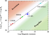 |
Fig. 1 Correlation among the star magnetic dipole μ (in Gauss cm3 units) estimated with different methods (unrelated to the accretion theory) and a combination of stellar parameters P7∕3 R (P in s and R in units of 106 cm) at the observationally determined luminosity at which the outburst light curves shows a knee or a drop (Lmin in erg s−1). We indicated LMXBs with red triangles, HMXBs with green squares, white dwarfs in intermediate polars with blue dots, and YSOs with cyan stars. The continuous line represents the best fit power law relation and separates the region where unimpeded matter accretion onto the star surface takes place from the region where it is halted (partially or completely) by the propeller mechanism. |
3 Observations and results: neutron stars
In this section we discuss in some detail the accreting magnetic neutron stars in high and low mass X-ray binaries which are in our sample. Special attention is given to the determination of the magnetic fields. In particular, the magnetic field strength for the two accreting millisecond pulsars in LMXBs is derived from the radio-pulsar spin-down measured during quiescence (Hartman et al. 2009; Papitto et al. 2013) and for the four HMXBs from the cyclotron resonant scattering features in their X-ray spectra (Tsygankov 2016).
3.1 SAX J1808.4–3658
SAX J1808.4–3658, the first accreting millisecond pulsar discovered (Wijnands & van der Klis 1998), has a spin period of 2.5 ms. The magnetic moment was estimated by interpreting the spin-down during quiescence as being due to rotating magnetic dipole radiation; this gave μ = 9.4 × 1025 G cm3 (Hartman et al. 2009). Other methods have been suggested in the literature, but all of them involve the magnetospheric radius and so are not relevant to the present study. We note, however, that the value of μ obtained through these estimates is broadly consistent with the value derived from rotating magnetic dipole radiation. Errors and values have been symmetrised in log scale for fitting purposes, and we adopted log(μ/G cm3) =  .
.
Gilfanov et al. (1998) after the discovery outburst already noted a fast dimming of the source around a luminosity of ~5 × 1035 erg s−1. Swift monitoring observations of the 2005 outburst led Campana et al. (2008) to estimate a limiting 0.3–10 keV luminosity of (2.5 ± 1.0) × 1035 erg s−1 by taking the lowest value during outburst and the luminosity of the rebrightenings. Using the broad-band Suzaku spectrum during outburst (Cackett et al. 2009), we estimated a bolometric correction of 1.7, giving a 0.1–100 keV limiting luminosity of log(Llim/erg s−1) =  .
.
3.2 IGR J18245–2452
IGR J18245–2452 is a transitional pulsar, the only one so far found to alternate between the accretion powered regime and the millisecond radio-pulsar regime (Papitto et al. 2013). IGR J18245–2452 lies in the M28 globular cluster at 5.5 kpc. The spin period is 3.9 ms (Papitto et al. 2013). Also in this case the magnetic field can be derived from the spin-down in the radio-pulsar regime. However, the period derivative is known with a large uncertainty and it is likely affected by the source acceleration in M28. Ferrigno et al. (2014) set a limit on the magnetic field to (0.7– 35) × 108 G. This resultsin a magnetic dipole moment of log(μ/G cm3) =  . The Swift monitoring of the 2013 outburst showed a steepening in the X-raylight curve around a 0.5–10 keV luminosity of ~1036 erg s−1 (Linares et al. 2014). An XMM-Newton observation caught IGR J18245–2452 continuously switching between a low and a high intensity state, with flux variations of a factor of ~100 on timescales of a few seconds (Ferrigno et al. 2014). This behaviour was interpreted in terms of centrifugal inhibition of accretion. Pulsations have also been detected at lower luminosities, though with pulse fraction decreasing with luminosity. On the contrary at higher luminosities the pulse fraction remained nearly constant. By adopting a bolometric correction of 2.5 based on spectral fits, we derived a limiting 0.1–100 keV luminosity of log(Llim/erg s−1) =
  .
.
3.3 GROJ1744–28
GRO J1744–28 is a peculiar transient bursting pulsar discovered close to the Galactic centre (Kouveliotou et al. 1996). It has a pulse periodof 0.467 s (Finger et al. 1996). The magnetic field has been directly estimated from an absorption cyclotron feature at Ecyc ~ 4.7 ± 0.1 keV in the X-ray spectrum with a hint of higher order harmonics (D’Aí et al. 2015; see also Doroshenko et al. 2015 who found a slightly lower line energy at ~4.5 keV). Its centroid energy is related to the magnetic field through  keV, where z is the gravitational redshift at the neutron star surface. Here and throughout this work we assume values of
  and 10 km for the mass and radius of the neutron star, respectively.For these values the gravitational redshift is z = 0.21, and a magnetic field of B = (4.9 ± 0.1) × 1011 G is derived, corresponding to a magnetic dipole moment of log(μ/G cm3) =
  . GRO J1744–28 is likely associated with the Galactic centre population at a distance of 8 kpc. A drop in the X-ray flux of a factor of ~10 and the disappearance of the pulsed signal in the RXTE data were interpreted by Cui (1997) as the onset of the propeller regime. The 2–60 keV absorbed limiting flux has been estimated as ~2.3 × 10⁻⁹ erg cm−2 s−1. Given the power law spectrum provided by Cui (1997, 1998), we derive a bolometric correction of 1.5 for the 0.1–100 keV unabsorbed flux. This results in a limiting luminosity of log(Llim/erg s−1) ~ 37.4.
This result is, however, subject to possible systematic uncertainties due to the high crowding in the Galactic centre region observed by the non-imaging RXTE proportional counter array. To improve on this, we take advantage of the deep monitoring of GRO 1744–28 carried out with the Swift satellite (Gehrels et al. 2004) during the 2014 outburst. The Swift/XRT (Burrows et al. 2005) light curve can be found in Fig. 2 (which was derived through the Leicester University automatic pipeline, Evans et al. 20092). During the main phase of the outburst the light curve was affected by a large number of bright bursts that characterise the “bursting pulsar” GRO 1728–44. These bursts ceased abruptly when the count rate decreased below ~20 c s−1. After a few days the periodic pulsations, which had a pulsed fraction of 10 ± 2% (90% confidence level), also dropped to < 8% (see Table 1). Fitting the pulsed fraction before and after obsid. 00030898054 (see Table 2) with the same value, results in an unacceptable fit (3 σ). Fitting the outburst light curve with a (phenomenological) Gaussian model, from the peak to the time when the pulsations become undetectable, shows that at later times there is a hint of a steeper turn off of the observed rate than model extrapolation (a Lorentzian or an exponential function provides poorer fits). Together with the disappearance of bursting activity and of X-ray pulsations, this can be taken as an indirect evidence for the propeller onset, even though differences from the abrupt turn off observed in other systems are apparent.
We estimate the limiting luminosity from the Swift spectrum of the first observation when no pulsations are detected (Obsid. 00030898054, see Table 1). The source spectrum was extracted with a 20 pixel radius circle, whereas the background spectrum was extracted at the edge of the window timing (WT) strip. Energy-resolved data were rebinned to 1 count per channel and fitted with an absorbed power law model by using C-statistics. We found NH = (9.8 ± 1.1) × 1022 cm−2 and a hard power law with Γ = 1.2 ± 0.2, consistent with previous estimates (Younes et al. 2015). The 0.3–10 keV unabsorbed flux is 9.5 ×10⁻¹⁰ erg cm−2 s−1, which, extrapolated to the 0.1–100 keV range, results in log(Llim/erg s−1) =  , a factor of 3lower than that estimated by Cui (1997).
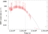 |
Fig. 2 Swift/XRT light curve of the 2014 outburst of GRO 1744–28. Variations in the XRT count rate along each observation are apparent, and the strong flares are due to Type II burst activity (thought to be due to accretion instability at the magnetosphere). The continuous line shows a Gaussian fit to the first part of the outburst (excluding the flaring activity). This fit does not apply to the latest stages of the outburst, which display a steeper decay. The dashed vertical line marks the time at which Type II bursting activity disappeared. The dotted vertical line marks the time at which pulsations were not detected. |
Swift/XRT observation log for GRO J1744–28.
3.4 4U 0115+63
4U 0115+63is a well-known hard X-ray transient binary, hosting a 3.61 s spinning neutron star orbiting an O9e companion (V635 Cas; Rappaport et al. 1978). Cyclotron features were observed in the X-ray spectrum during outbursts (White et al. 1983); four cyclotron harmonics were revealed during a BeppoSAX observation, resulting in a precise determination of the fundamental cyclotron line energy of Ecyc = 12.74 ± 0.08 keV (Santangelo et al. 1999). Using the same redshift as before, this converts to a magnetic moment of log(μ/G cm3) =
 . The distance was estimated to be ~7 kpc (Negueruela et al. 2001). 4U 0115+63 showed a very large variation during a long BeppoSAX observation (a factor of ~250 in 15 h; Campana et al. 2001), which was interpreted in terms of the action of the centrifugal barrier. A knee was present in the rising phase (see Fig. 2 intervals 2 and 3 in Campana et al. 2001) from which we estimate a limiting luminosity in the 0.1–100 keV of log(Llim/erg s−1) =
  . Our estimate is consistent with the one by Tsygankov (2016) evaluated through a drop in the Swift/XRT light curve of the 2015 outburst, even though the latest stages of the outburst were not well sampled.
3.5 V 0332+53
V 0332+53 is a hard X-ray transient similar to 4U 0115+63. The companion is an O8-9e-type main sequence star at a distance of ~7 kpc (Negueruela et al. 1999). The neutron star spin period is 4.4 s (Doroshenko et al. 2016). Cyclotron line features were discovered by Makishima et al. (1990). Detailed studies carried out with RXTE and INTEGRAL revealed up to two higher harmonics and a fundamental line energy between 25–27 keV depending on the modelling (Kreykenbohm et al. 2005; Pottschmidt et al. 2005). This leads to a redshift corrected magnetic dipole moment log(μ/G cm3) =
 . Stella et al. (1986) were the first to find signs of centrifugal inhibition of accretion in the outburst decay of V 0332+53. A detailed analysis by Tsygankov (2016) of the 2015 outburst decay with Swift/XRT showed a rapid turn off at a limiting luminosity of log(Llim/erg s−1) =
  (0.1–100 keV).
3.6 SMC X-2
The Small Magellanic Cloud (d = 62 kpc) hosts a large number of Be-star X-ray binaries. One of them, SMC X-2, has a short spin period of 2.37 s (Corbet et al. 2001). NuSTAR and Swift simultaneous observations showed the presence of a cyclotron line feature at 28 ± 1 keV (Jaisawal & Naik 2016). This leads to a redshift corrected magnetic dipole moment log(μ/G cm3) =
 . A dense Swift/XRT monitoring of the recent 2016 outburst (Lutovinov et al. 2017) reveals a steepening in the outburst light curve at a luminosity of ~4 × 1036 erg s−1. Assuming a correction factor of 1.5 to account for our lower energy bound (from 0.5 to 0.1 keV), we obtain log(Llim/erg s−1) =
  .
.
3.7 Other sources
We note that the abrupt X-ray flux drop of more than a decade in minutes to hours that was observed in several HMXB pulsators with spin periods in the ~100 s range was ascribed to a sudden decrease in the density of the companion’s wind from which they accrete (Vela X-1, Kreykenbohm et al. 2009; GX 301-2, Göğüş et al. 2011; 4U 1907+09, Doroshenko et al. 2012); therefore, we did not include these sources in our sample. Other HMXBs for which the magnetic field was measured from cyclotron line features possess a spin period that is too long to propel the inflowing matter away during any stage of their outbursts.
The two transitional millisecond X-ray pulsars PSR J1023+0038 (Archibald et al. 2009) and XSS J12270–4859 (de Martino et al. 2013; Bogdanov et al. 2015; Roy et al. 2015), which have known spin periods, magnetic fields, and distances, have not yet displayed an X-ray outburst and therefore are not included in the sample.
4 Observations and results: white dwarfs
Accreting magnetic white dwarfs are usually classified as intermediate polars and polars depending on the strength of the magnetic field and, in turn, whether or not a disc forms. The white dwarf magnetic field in polars is strong enough to prevent the formation of an accretion disc and they do not display outbursts. On the other hand, a small number of intermediate polars display dwarf nova-like outbursts. These sources are generally short orbital period systems (i.e. Porb < 2 h) except for GK Per (Porb ~48 h) and very few others. We selected 68 intermediate polars from Mukai’s web page3 , including all sources flagged as probable, confirmed, and ironclad. We further down-selected these by keeping only white dwarfs with known spin period, mass, and distance estimates. Radii were computed from  (Nauenberg 1972).
Magnetic fields are difficult to measure due to the lack of detectable optical/near-IR polarisation in the majority of IPs. A few of them were found to be polarised with loosely estimated B-fields ~(4–30) × 106 G (see Ferrario et al. 2015 and references therein). We therefore assume a conservative upper limit of 4 × 10⁶ G for the systems under study simply because none of the sources under the present analysis has shown hints of optical/near-IR polarisation yet.
A lower limit cannot be easily worked out. A non-negligible magnetic field is needed since the emission is pulsed and thus matter is channeled onto the poles. Based on this we considered two intermediate polars showing pulsed emission in X-rays at high luminosities: YY (DO) Dra (Szkody et al. 2002) and GK Per (Yuasa et al. 2016). From the best bremsstrahlung model fitting of the X-rayspectrum of these sources we derived the density of the accreting material (assuming a conservative column height of the order of the stellar radius). Then, equating the thermal pressure to the magnetic pressure we derived a magnetic field in excess of ~105 G in both cases. The same value is obtained by calculating the limiting magnetic field for which column-like accretion would still occur over the entire white dwarf surface (Frank et al. 2002). Therefore we conservatively assume B > 105 G as a lower limit for the magnetic field in intermediate polars.
4.1 WZ Sge
WZ Sge is a dwarf nova showing regular outbursts with a recurrence period of ~30 yr. It shows super-outbursts (7 mag amplitude) with characteristic reflaring at the end of the primary event. WZ Sge has an orbital period of 81.6 min and lies at a distance of 43 pc based on parallax measurements. The mass of the white dwarf is  (Steeghs et al. 2007). Several oscillations around 28 s have been discovered in the optical. Optical observations in quiescence revealed a 27.87 s signal that was phase stable from night to night (Patterson 1980). In addition a signal at the same period was detected in the 2–6 keV range from ASCA data, but not in previous X-ray observations (Patterson et al. 1998), which likely represents the white dwarf spin period. WZ Sge is a good candidate IP (Lasota et al. 1999). A distinctive knee in the 2001 outburst light curve was observed around V ~11 (Kato et al. 2009). Ultraviolet observations allowed an order of magnitude estimate of the mass accretion rate before and after the time of the transition. During the plateau phase, before the occurrence of the knee, the mass accretion rate was
  yr−1 (Long et al. 2003), whereas it was
  yr−1 at the peak of the first rebrightening, close in magnitude to the occurrence of the knee (Godon et al. 2004). Taking the mean value of these two estimates and increasing the error by a factor of two, we end up with log(Llim/erg s−1) =
  .
.
It is important to note that WZ Sge is the prototype of a subclass of dwarf novae characterised by optical light curves which display large outbursts, followed by a knee in the decay phase and subsequent rebrightenings (Kato 2015). WZ Sge is one of the few members of this class for which the spin period has been inferred.
Despite other interpretations of dimmings and rebrightenings during dwarf nova outburst decays (e.g. Meyer & Meyer-Hofmeister 2015; Hirose & Osaki 1990), which can still occur but in the end will produce a decrease in the mass inflow rate and in turn the onset of the propeller, here the inference of our work is that all WZ Sge-type binaries should host a fast spinning white dwarf. Based on the knee luminosity and magnetic field in the above-described range, we expect spin periods in the 10–500 s range.
4.2 V455 And
V455 And (also known as HS 2331+3905) is a unique cataclysmic variable that was discovered in the Hamburg Quasar Survey. Partial eclipses in the optical light curve recur at the orbital period of 81.1 min. A stable period at 67.62 s was found in quiescent optical data, which is interpreted as the spin period of the white dwarf (Bloemen et al. 2012). Modelling the quiescent far-UV emission of the white dwarf leads to a distance of 90 pc (Araujo-Betancor et al. 2005). No firm estimate of the mass has been obtained; we assumed  , the same value used to fit the far-UV spectrum.
In 2007 September, V455 And increased its brightness by 8 mag, similar to the outburst amplitudes observed in WZ Sge stars. A step-like (2 mag) decrease was observed ~20 d after the beginning of the outburst when V455 And had V = 12.7. Multifilter observationsallowed Matsui et al. (2009) to estimate a temperature of (10–12) × 103 K at the transition, and we derive a bolometric correction of a factor of 10 with respect to the observed V magnitude.
4.3 HT Cam
HT Cam is a cataclysmic variable with a short orbital period (81 min). Its 515.1 s spin period was found from optical photometricand X-ray data (Kemp et al. 2002). Following de Martino et al. (2005), we assume a white dwarf mass of  and a distance of 100 pc.
HT Cam shows rare and brief outbursts from V ~ 17.8 to V ~ 12–13. One of these outbursts was monitored in detail in 2001 by Ishioka et al. (2002). After a short plateau, HT Cam showed a dramatic decline of more than 4 mag d−1. The declinerate changed around V ~ 14, when pulsations also became less pronounced (Ishioka et al. 2002). It is difficult to derive the luminosity at the turning point since the transition to quiescence was extremely rapid (a few days) and no multiwavelength data are available. We therefore consider the bolometric quiescent luminosity as derived from the X-ray band of 9 × 1030 erg s−1 (de Martino et al. 2005) and correct it for the luminosity change in the optical by 3.8 mag. We adopt in this case a total error of an order of magnitude (Table 1).
4.4 AE Aqr
AE Aqr is an intermediate polar which hosts one of the fastest known white dwarfs (33 s spin period) in an IP system (Patterson 1979).
It shows a peculiar phenomenology, with strong broad-band variability from the radio to X-ray and possibly TeV energies. Doppler tomography based on optical spectra showed an irregular accretion pattern that has been interpreted as arising from the action of the propeller mechanism (Wynn et al. 1997). The distance is ~100 pc (based on HIPPARCOS data) and the mass has been estimated to be  (Casares et al. 1996). Estimates for the magnetic field are uncertain. Values in the (0.3–30) × 106 G have been obtained, as summarised by Li et al. (2016). The X-ray luminosity of 1031 erg s−1, provides a reasonable estimate of the bolometric luminosity (Oruru & Meintjes 2012; see also the recent Swift/XRT+NuSTAR estimate Kitaguchi et al. 2014, Table 3).
4.5 Other sources
There are a number of other IPs which do not display hints of a knee in their outburst light curve decay (see Tables 1 and 3). Consequently, we assume that their quiescent emission is powered by accretion onto the white dwarf surface and adopt the corresponding luminosity as an upper limit to Llim. Figure 3 shows these upper limits plotted together with the points in Fig. 1; all of them are consistent with the propeller line, while others are close to it (Table 4).
Owing to insufficient data (convincing distance, mass estimates, and more importantly a sound bolometric correction for the knee luminosity), CC Scl was not included in our sample even though it showed a drop in flux that could be due to the action of the propeller.
Summary table for white dwarfs in confirmed IPs with smooth outburst declines, providing upper limits.
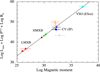 |
Fig. 3 As in Fig. 1. We have included here a few upper limits from WDs in IPs close to the propeller line (orange upper limits), and one source (AE Aqr) considered to persistently lie in the propeller regime (grey lower limit). The upper and lower limits are displayed to show the consistence with the relation, but they were not used in the fit. |
White dwarf parameters.
5 Observations and results: young stellar objects
Young stellar objects (YSOs) are often surrounded by an accretiondisc formed by matter infalling from the parent cloud. A small number of these low mass pre-main sequence stars show large outbursts or eruptions of several magnitudes, signifying episodes of enhanced mass accretion rate. Based on their properties, they are classified as FUors (named after the prototype of this class FU Ori), which display violent and probably recurrent outbursts about once per century, and EXors (EX Lup ancestor), which show shorter duration (weeks to months) and less pronounced irregular outbursts several times in a decade (Hartman et al. 2016; Audard et al. 2014). FUors and EXors are relatively rare; for only one YSO, V1647 Ori, we could find all values that are needed for our study. EX Lup itself might have shown a steep drop in flux at the end of the 2008 outburst, but the steepening did not have a knee; instead its light curve morphology resembles the dip-like structure seen in nova outburst from DQ Her and likely caused by the formation ofdust. FU Ori initiated a major outburst from 15–16 mag to about 10 mag over several months in 1936 with a very slow decay and no sign of a turn off. The mass accretion rate increased by 2–3 orders of magnitude (Beck & Aspin 2012); therefore, we did not include these YSOs in our sample.
5.1 V1647 Ori
V1647 Ori is an eruptive YSO in Orion. It showed several outbursts that do not share the timescales and amplitudes of EXors. Evidence for accretion were clearly found in spectroscopic data as testified by the Br γ emission line (Brittain et al. 2010). It went into outburst in 2004–2006 and then again in 2008. Together with an increase in the optical and near-IR magnitudes, V1647 Ori displayed a correlated bright outburst in the X-ray band (Teets et al. 2011). Based on X-ray outburst data Hamaguchi et al. (2012) detected a 1 d periodicity, identified as the protostar rotation at near break-up speed. The emission is interpreted as originating at the magnetic footprints of an accretion flow governed by magnetic reconnection. The shape of the 1 d X-ray periodicity was found to be consistent with the modulation expected from two antipodal hot spots, suggesting that accretion took place through a mainly dipolar field geometry (see Appendix A). Therefore, rotation takes place at near break-up speed in V1647 Ori. In order to confine the 50 MK plasma, as derived from X-ray spectral fits, a magnetic field of at least 100 G must be invoked (Hamaguchi et al. 2012). As an upper limit on B we take the mean field measured in isolated YSOs of 3 × 10³ G (Johns-Krull 2007). Based on pre-outburst bolometric luminosity and stellar temperature, Aspin et al. (2006) estimated a mass of  and a radius of
  for V1647 Ori at a distance of 400 pc.
V1647 Ori emits preferentially in the near-IR. The H-band light curve showed a clear steepening at a luminosity of ~8 × 1032 erg s−1 (Teets et al. 2011). However, the luminosity at the knee is not easy to estimate. In addition, V1647 Ori is heavily absorbed. We started from the estimate of the mass accretion rate during quiescence of  yr−1 based on the flux of the Br γ emission line (Acosta-Pulido et al. 2007). By using the same method for the outburst maximum, Acosta-Pulido et al. (2007) derived a peak mass accretion rate of
  yr−1. A factor of ~10 variation in the mass inflow rate is in agreement with the H-band light curve, which showed an enhancement of a factor of ~10 in the near-IR flux (Hamaguchi et al. 2012). Given that the knee occurred close to the middle of the light curve in log scale, we took the logarithmic mean between the two mass accretion rates (quiescent and peak outburst) and converted it to a bolometric luminosity by using G M Ṁ∕R. A logarithmic error of ± 0.3 was assumed (see Table 1).
6 A universal relation for the limiting luminosity
The values of Llim obtained from our sample span about 5 decades; they are listed in Table 1 (see also Fig. 1). We carried out a parametric search in order to determine the dependence of Llim on the star’s parameters and test the theory of disc-magnetosphere interaction. We adopt a general relation of the form
 (4)
similar to Eq. (3) but with free exponents to be derived from the fit to the observational data. We performed a grid search on α, β, and γ over the interval from 0 to 4 for each parameter, a larger range than envisaged in all models. We also included a fixed mass dependence to the − 2∕3 power (as in Eq. (3)) because the relatively small range of stellar masses (less than a factor of 3, spanning
(4)
similar to Eq. (3) but with free exponents to be derived from the fit to the observational data. We performed a grid search on α, β, and γ over the interval from 0 to 4 for each parameter, a larger range than envisaged in all models. We also included a fixed mass dependence to the − 2∕3 power (as in Eq. (3)) because the relatively small range of stellar masses (less than a factor of 3, spanning  ) does not allow us to test this dependence independently. We proceeded as follows: we selected a value on the grid of the exponents, establish the best fitting relation, i.e. determine k, and took note of the χ2 of the fit. Based on this grid search, we found the best fit (reduced χ2 = 0.97 for 9 degrees of freedom) and determined the 90% confidence intervals for three interesting parameters. We obtained
  ,
,  , and
, and  (we note that there is an almost linear correlation between α and β, which is accounted for in the evaluation of the errors). The values of all parameters are consistent with the dependence predicted bysimple disc-magnetosphere interaction theory (Eq. (3)) over a very wide range of objects and physical occurrences.
We can also use our sample with exponents fixed at α =2, β =7∕3, and γ = 1 in order to evaluate the ξ parameter from the best fit value of k (see Eqs. (3) and (4)). We obtain ξ = 0.49 ± 0.05 (1 σ), a value consistent with that predicted in some disc-magnetosphere models4 (Ghosh & Lamb 1979; Wang 1987). We note that the precision attained in the determination of the parameters stems from the very wide range of magnetic dipole moments (> 10 decades), spin periods (>7 decades), and star radii (>5 decades) in our sample. We thus conclude that our study provides the most extensive observational confirmation of basic theory for the accretion disc-magnetosphere interaction.
In deriving our conclusions we implicitly assumed that the same accretion disc-magnetosphere interaction holds for different astrophysical objects, an approach adopted in other studies (Romanova & Owocki 2016 and references therein). Even if we cannot prove this assumption, our findings are consistent with different classes of sources in our sample behaving similarly and in a consistent manner with the propeller mechanism (see Sect. 3).
An entirely different scenario based on a DIM has been widely adopted to model the flux drops observed in the outburst decay of black hole transients (and dwarf novae)5. The disc mass inflow rate decreases on an exponential decay timescales of a few weeks,  d (Rh,11 the maximum hot-state disc radius in units of 1011 cm; King & Ritter 1988). In these systems the matter proceeds unimpeded all the way to the compact object. After the transition to the cold state the outburst light curves should show a characteristic “brink” (i.e. a knee), followed by a linear decay (Powell et al. 2007).
In the best sampled light curves the decay after the knee is not linear but exponential (e.g. Aql X-1, Campana et al. 2014 or 4U 0115+63, Campana et al. 2001). Campana et al. (2013) studied 20 outbursts from Aql X-1, showing that the brink when detectable always occurred at a luminosity larger than the knee luminosity. Unfortunately, the less sampled sources cannot clearly reveal these differences.
The decrease in luminosity across the knee in the HMXBs (e.g. V 0332+53 and 4U 0115+63, which have spins of several seconds and rcor ≫ R) is ~102, whereas it is much smaller in LMXBs, CVs, and YSOs (where rcor is only a few times R). This has no obvious interpretation in the DIM, where the luminosity swing is determined only by the accretion rate in the two states of the disc; on the contrary, it is naturally interpreted by the propeller model, where the luminosity swing is expected to scale approximately6 as rcor∕R (Corbet 1996; Campana et al. 1998).
Moreover, if the sharp decay in the light curve of one or more of our sources were due to the DIM (or to some other mechanism that does not block the matter flow), the corresponding points would be in the red region above the correlation line in Fig. 1. We do not observe any obvious outliers confirming that our interpretation applies to most if not all sources in our sample.
The fact that the relation expressed in Eq. (4) (derived from the correlation in Fig. 1) corresponds approximately to the condition rm ~ rcor also indicates that the present-day values of the star’s spin and magnetic field have been largely determined by its accretion history (and consequent spin-up/spin-down torques and/or B-field decay) over evolutionary timescales. Therefore, the correlation itself cannot result from angular momentum or magnetic flux conservation in the star’s progenitor.
Given our parametrisation of Eq. (4) we can rewrite the magnetospheric radius (Eq. (1)) as
 (5)
which is independent of the central mass object. For standard accretion theory values α = 2, β =7∕3, and γ = 1 we derive
(5)
which is independent of the central mass object. For standard accretion theory values α = 2, β =7∕3, and γ = 1 we derive
 (6)with L36 the accretion luminosity in units of 1036 erg s−1. Equation (3) instead becomes
 (7)
(7)
7 Conclusions
We determined the critical luminosity at which the transition from accretion to propeller regime occurs in a number of transient neutron stars, white dwarf, and young stellar objects, whose spin period, radius, and magnetic field are observationally measured (or constrained). The transition luminosity was estimated on a pure observational basis as the luminosity at which the outburst light curve shows a distinctive knee. This allowed us to probe the dependence of this critical luminosity on the star’s main parameters, independently of the accretion theory. We found good agreement of the best fit indices and those predicted by accretion theory if the knee arises from the transition to the propeller regime.
The observationally tuned Eq. (3), together with the value of ξ ≃ 0.5 that we determined, adds confidence and precision to previous studies exploiting the knee associated to the onset of the centrifugal barrier to infer (or constrain) the magnetic field of accreting neutron stars of known spin period. For instance the magnetic field of the prototypical LMXB transient, Aql X-1, can be estimated as μ = (5.7 ± 0.3) × 1026 G cm3(at 4.5 kpc) based on the luminosity of the knee observed in the outburst light curves in 2010 and 2014 (Campana et al. 2014). The same is true for a number of fast spinning neutron stars in HMXBs in the Magellanic Clouds (Christodoulou et al. 2016). Moreover Eq. (3) extends the applicability of the method and its predictive power to other classes of objects, notably magnetic white dwarfs in CVs and YSOs. There is an emerging class of short orbital period dwarf novae showing steep decays in their optical light curves, often followed by rebrightenings. These are known as WZ Sge dwarf novae (Kato 2015). The prototypical source, WZ Sge, is also a candidate IP occasionally displaying fast pulsations at 28 s. For all sources of this class we predict similar characteristics, i.e. a magnetic field in the 105–106 G range and a fast spin period in the 10–500 s range. In the study of FUor and EXor, drops in the near-IR light curves, coupled with estimates of the spin period based on X-ray and optical/near-IR polarimetry, will provide a new tool for evaluating their magnetic fields.
Acknowledgments
We thank F. Coti Zelati, P. D’Avanzo, T. Giannini, D. Lorenzetti, and B. Nisini for useful conversations. DDM and LS acknowledge support from ASI-INAF contract I/037/12/0. Swift is a NASA mission with participation of the Italian Space Agency and the UK Space Agency. This research has made use of software and tools provided by the High Energy Astrophysics Science Archive Research Center (HEASARC), which is a service of the Astrophysics Science Division at NASA/GSFC and the High Energy Astrophysics Division of the Smithsonian Astrophysical Observatory. This work has made use of data supplied by the UK Swift Science Data Centre at the University of Leicester.
Appendix A Multipole magnetic fields
Virtually allmodels of the disc-magnetospheric interaction, assume thatthe star’s magnetic field is dipolar. The possibility that only higher multipole components are present can be ruled out since the dependence on the parameters in Eq. (1) would be inconsistent with the values that we determined. For instance, for a pure quadrupolar field it would have a radial dependence Bq ~ μq∕r5, where μq is the magnetic quadrupole moment. The expected scaling of the magnetospheric radius in this case would be  (Vietri & Stella 1998). This is excluded by our analysis (see Sect. 6).
An implicit requirement of our study is that the dipolar component dominates not only at the disc-magnetosphere boundary, but also at the radius where the magnetic field value is estimated (even if higher multipole components were present, the dipole would still dominate at large radii by virtue of its weaker radial dependence). Among neutron stars only magnetars and a few accreting pulsars in ultraluminous X-ray sources are believed to feature conspicuous higher multipole components at the star surface (Tiengo et al. 2013; Israel et al. 2017). However, no evidence for such components has ever been found in the HMXB neutron stars in our sample, for which the magnetic field is estimated through cyclotron resonant features. A quadrupolar magnetic field component has been suggested for Her X-1 to model the complex pulse profile (Panchenko & Postnov 1994); however, its contribution to the magnetic field should be only ~ 30% (Klochkov et al. 2008) at the neutron star surface (as measured from the cyclotron line) and negligible at the magnetospheric radius (which is ~ 108 cm farther away). Only a weak dipolar magnetic field is expected to survive in the fast spinning neutron stars of LMXBs. The magnetic field estimate that we adopt is based on the spin-down torque in the quiescent (no-accretion) phase and thus it exclusively involves the dipole component of the field. Higher magnetic multipole components are observed in young white dwarfs, but in older systems like short period binaries (≳ 1 Gyr) a substantial decay of multipolar components is expected (Beuermann et al. 2007). In YSOs surface magnetic fields which comprise contributions from higher magnetic multipoles have been found (Johns-Krull 2007). However, in the case of V1657 Ori the shape of the rotationally modulated X-ray light curve argues in favour of magnetic accretion through a dipole-dominated field.
We thus conclude that our assumption that the magnetic dipole dominates over higher multipole components appears to be well justified for the objects in our sample.
References
- Acosta-Pulido, A. J., Kun, M., Ábrahám, P., et al. 2007, AJ, 133, 2020 [NASA ADS] [CrossRef] [Google Scholar]
- Araujo-Betancor, S., Gänsicke, B. T., Hagen, H.-J., et al. 2005, A&A, 430, 629 [NASA ADS] [CrossRef] [EDP Sciences] [Google Scholar]
- Archibald, A. M., Stairs, I. H., Ransom, S. M., et al. 2009, Science, 324, 1411 [NASA ADS] [CrossRef] [PubMed] [Google Scholar]
- Aspin, C., Barbieri, C., Boschi, F., et al. 2006, AJ, 132, 1298 [NASA ADS] [CrossRef] [Google Scholar]
- Audard, M., Ábrahám, P., Dunham, M. M., et al. 2014, in Protostars and Planets VI, eds. H. Beuther, R. S. Klessen, C. P. Dullemond, & T. Henning (Tucson: University of Arizona Press), 387 [Google Scholar]
- Barlow, E. J., Knigge, C., Bird, A. J., et al. 2006, MNRAS, 372, 224 [NASA ADS] [CrossRef] [Google Scholar]
- Beck, T. L., & Aspin, C. 2012, AJ, 143, 55 [Google Scholar]
- Beuermann, K., Euchner, F., Reinsch, K., Jordan, S., & Gänsicke, B. T. 2007, A&A, 463, 647 [NASA ADS] [CrossRef] [EDP Sciences] [Google Scholar]
- Bloemen, S., Marsh, T. R., Degroote, P., et al. 2012, MNRAS, 429, 3433 [NASA ADS] [CrossRef] [Google Scholar]
- Bogdanov, S., Archibald, A. M., Bassa, C., et al. 2015, ApJ, 806, 148 [NASA ADS] [CrossRef] [Google Scholar]
- Brittain, S. D., Rettig, T. W., Simon, T., Gibb, E. L., & Liskowsky, J. 2010, ApJ, 708, 109 [NASA ADS] [CrossRef] [Google Scholar]
- Burrows, D. N., Hill, J. E., Nousek, J. A., et al. 2005, Space Sci. Rev., 120, 165 [NASA ADS] [CrossRef] [Google Scholar]
- Cackett, E. M., Altamirano, D., Patruno, A., et al. 2009, ApJ, 694, L21 [NASA ADS] [CrossRef] [Google Scholar]
- Campana, S., Colpi, M., Mereghetti, S., Stella, L., & Tavani, M. 1998, A&ARv, 8, 279 [NASA ADS] [CrossRef] [Google Scholar]
- Campana, S., Gastaldello, F., Stella, L., et al. 2001, ApJ, 561, 924 [NASA ADS] [CrossRef] [Google Scholar]
- Campana, S., Stella, L., & Kennea, J. A. 2008, ApJ, 684, L99 [NASA ADS] [CrossRef] [Google Scholar]
- Campana, S., Coti Zelati, F., & D’Avanzo, P. 2013, MNRAS, 432, 1695 [NASA ADS] [CrossRef] [Google Scholar]
- Campana, S., Brivio, F., Degenaar, N., et al. 2014, MNRAS, 441, 1984 [NASA ADS] [CrossRef] [Google Scholar]
- Campbell, C. G. 2011, MNRAS, 414, 3071 [NASA ADS] [CrossRef] [Google Scholar]
- Casares, J., Mouchet, M., Martinez-Pais, I.G., & Harlaftis, E.T. 1996, MNRAS, 282, 182 [NASA ADS] [CrossRef] [Google Scholar]
- Christodoulou, D. M., Laycock, S. G. T., Yang, J., & Fingerman, S. 2016, ApJ, 829, 30 [NASA ADS] [CrossRef] [Google Scholar]
- Corbet, R. H. D. 1996, ApJ, 457, L31 [NASA ADS] [CrossRef] [Google Scholar]
- Corbet, R. H. D., Marshall, F. E., Coe, M. J., Laycock, S., & Handler, G. 2001, ApJ, 548, L41 [NASA ADS] [CrossRef] [Google Scholar]
- Cui, W. 1997, ApJ, 482, L163 [NASA ADS] [CrossRef] [Google Scholar]
- Cui, W. 1998, AIP Conf. Proc., 431, 405 [Google Scholar]
- D’Aí, A., Di Salvo, T., Iaria, R., et al. 2015, MNRAS, 449, 4288 [NASA ADS] [CrossRef] [Google Scholar]
- D’Angelo, C., & Spruit, H. C. 2012, MNRAS, 420, 416 [NASA ADS] [CrossRef] [Google Scholar]
- de Martino, D., Matt, G., Mukai, K., et al. 2005, li A&A, 437, 935 [NASA ADS] [CrossRef] [EDP Sciences] [Google Scholar]
- de Martino, D., Belloni, T., Falanga, M., et al. 2013, A&A, 550, A89 [NASA ADS] [CrossRef] [EDP Sciences] [Google Scholar]
- Doroshenko, V., Santangelo, A., Ducci, L., & Klochkov, D. 2012, A&A, 548, A19 [NASA ADS] [CrossRef] [EDP Sciences] [Google Scholar]
- Doroshenko, R., Santangelo, A., Doroshenko, V., Suleimanov, V., & Piraino, S. 2015, MNRAS, 452, 2490 [NASA ADS] [CrossRef] [Google Scholar]
- Doroshenko, V., Tsygankov, S., & Santangelo, A. 2016, A&A, 589, A72 [NASA ADS] [CrossRef] [EDP Sciences] [Google Scholar]
- Evans, P. A., Beardmore, A. P., Page, K. L., et al. 2009, MNRAS, 397, 1177 [NASA ADS] [CrossRef] [Google Scholar]
- Ferrario, L., deMartino, D., & Gänsicke, B. T. 2015, Space Sci. Rev., 191, 111 [NASA ADS] [CrossRef] [Google Scholar]
- Ferrigno, C., Bozzo, E., Papitto, A., et al. 2014, A&A, 567, A77 [NASA ADS] [CrossRef] [EDP Sciences] [Google Scholar]
- Finger, M. H., Koh, D. T., Nelson, R. W., et al. 1996, Nature, 381, 291 [NASA ADS] [CrossRef] [Google Scholar]
- Frank, J., King, A., & Raine, D. J. 2002, Accretion Power in Astrophysics, 3rd edn. (Cambridge: Cambridge University Press) [Google Scholar]
- Gehrels, N., Chincarini, G., Giommi, P., et al. 2004, ApJ, 611, 1005 [NASA ADS] [CrossRef] [Google Scholar]
- Ghosh, P., & Lamb, F. K. 1979, ApJ, 234, 296 [NASA ADS] [CrossRef] [Google Scholar]
- Gilfanov, M., Revnivtsev, M., Sunyaev, R., & Churazov, E. 1998, A&A, 338, L83 [NASA ADS] [Google Scholar]
- Godon, P., Sion, E. M., Cheng, F., et al. 2004, ApJ, 602, 336 [NASA ADS] [CrossRef] [Google Scholar]
- Göğüş, E., Kreykenbohm, I., & Belloni, T. M. 2011, A&A, 525, L6 [NASA ADS] [CrossRef] [EDP Sciences] [Google Scholar]
- Hamaguchi, K., Grosso, N., Kastner, J. H., et al. 2012, ApJ, 754, 32 [NASA ADS] [CrossRef] [Google Scholar]
- Hartman, J. M., Patruno, A., Chakrabarty, D., et al. 2009, ApJ, 702, 1673 [NASA ADS] [CrossRef] [Google Scholar]
- Hartmann, L., Herczeg, G., & Calvet, N. 2016, ARA&A, 54, 135 [NASA ADS] [CrossRef] [Google Scholar]
- Hayashi, T., & Ishida, M. 2014, MNRAS, 438, 2267 [NASA ADS] [CrossRef] [Google Scholar]
- Hirose, M., & Osaki, Y. 1990, PASJ, 42, 135 [NASA ADS] [Google Scholar]
- Hoard, D. W., Linnell, A. P., Szkody, P., & Sion, E. M. 2005, AJ, 130, 214 [NASA ADS] [CrossRef] [Google Scholar]
- Illarionov, A. F., & Sunyaev, R. A. 1975, A&A, 39, 185 [NASA ADS] [Google Scholar]
- Ishioka, R., Kato, T., Uemura, M., et al. 2002, PASJ, 54, 581 [NASA ADS] [Google Scholar]
- Israel, G. L. , Belfiore, A., Stella, L., et al. 2017, Science, 355, 817 [NASA ADS] [CrossRef] [Google Scholar]
- Jaisawal, G. K., & Naik, S. 2016, MNRAS, 461, L97 [NASA ADS] [CrossRef] [Google Scholar]
- Johns-Krull, C. M. 2007, ApJ, 664, 975 [NASA ADS] [CrossRef] [Google Scholar]
- Kato, T. 2015, PASJ, 67, 108 [NASA ADS] [CrossRef] [Google Scholar]
- Kato, T., Imada, A., Uemura, M., et al. 2009, PASJ, 61, S395 [NASA ADS] [Google Scholar]
- Kemp, J., Patterson, J., Thorstensen, J. R., et al. 2002, PASP, 114, 623 [NASA ADS] [CrossRef] [Google Scholar]
- King, A. R., & Ritter, H. 1988, MNRAS, 293, L42 [Google Scholar]
- Kitaguchi, T., An, H., Beloborodov, A. M., et al. 2014, ApJ, 782, 3 [NASA ADS] [CrossRef] [Google Scholar]
- Klochkov, D., Staubert, R., Postnov, K., et al. 2008, A&A 482, 907 [NASA ADS] [CrossRef] [EDP Sciences] [Google Scholar]
- Kluźniak, W., & Rappaport, S. 2007, ApJ, 671, 1990 [NASA ADS] [CrossRef] [Google Scholar]
- Kouveliotou, C., van Paradijs, J., Fishman, G. J., et al. 1996, Nature, 379, 799 [NASA ADS] [CrossRef] [Google Scholar]
- Kreykenbohm, I., Mowlavi, N., Produit, N., et al. 2005, A&A, 433, L45 [NASA ADS] [CrossRef] [EDP Sciences] [Google Scholar]
- Kreykenbohm, I., Wilms, J., Kretschmar, P., et al. 2009, ArXiv e-prints [arXiv:0903.0838] [Google Scholar]
- Landi, R., Bassani, L., Dean, A. J., et al. 2009, MNRAS, 392, 630 [Google Scholar]
- Lasota, J.-P. 2001, New Astron. Rev., 45, 449 [NASA ADS] [CrossRef] [Google Scholar]
- Lasota, J.-P., Kuulkers, E., & Charles, P. 1999, MNRAS, 305, 473 [NASA ADS] [CrossRef] [Google Scholar]
- Li, J., & Wickramasinghe, D. T. 1997, MNRAS, 286, L25 [NASA ADS] [CrossRef] [Google Scholar]
- Li, J., Torres, D. F., Rea, N., et al. 2016, ApJ, 832, 35 [NASA ADS] [CrossRef] [Google Scholar]
- Linares, M., Bahramian, A., Heinke, C., et al. 2014, MNRAS, 438, 251 [NASA ADS] [CrossRef] [Google Scholar]
- Long, K. S., Froning, C. S., Gänsicke, B., et al. 2003, ApJ, 591, 1172 [NASA ADS] [CrossRef] [Google Scholar]
- Lovelace, R. V. E., Romanova, M. M., & Bisnovatyi-Kogan, G. S. 1995, MNRAS, 275, 244 [NASA ADS] [CrossRef] [Google Scholar]
- Luna, G. J. M., Raymond, J. C., Brickhouse, N. S., Mauche, C. W., & Suleimanov, V. 2015, A&A, 578, A15 [NASA ADS] [CrossRef] [EDP Sciences] [Google Scholar]
- Lutovinov, A., Tsygankov, S., Krivonos, R., Molkov, S., & Poutanen, J. 2017, ApJ, 834, 209 [NASA ADS] [CrossRef] [Google Scholar]
- Makishima, K., Mihara, T., Ishida, M., et al. 1990, ApJ, 365, L59 [NASA ADS] [CrossRef] [Google Scholar]
- Matsui, R., Uemura, M., Arai, A., et al. 2009, PASJ, 61, 1081 [NASA ADS] [CrossRef] [Google Scholar]
- Meyer, F., & Meyer-Hofmeister, E. 2015, PASJ, 67, 52 [NASA ADS] [CrossRef] [Google Scholar]
- Nauenberg, M. 1972, ApJ, 175, 417 [NASA ADS] [CrossRef] [Google Scholar]
- Negueruela, I., Roche, P., Fabregat, J., & Coe, M. J. 1999, MNRAS, 307, 695 [NASA ADS] [CrossRef] [Google Scholar]
- Negueruela, I., Okazaki, A. T., Fabregat, J., et al. 2001, A&A, 369, 117 [NASA ADS] [CrossRef] [EDP Sciences] [Google Scholar]
- Nelson, R. W., Bildsten, L., Chakrabarty, D., et al. 1997, ApJ, 488, L117 [NASA ADS] [CrossRef] [Google Scholar]
- Oruru, B., & Meintjes, P. J. 2012, MNRAS, 421, 1557 [NASA ADS] [CrossRef] [Google Scholar]
- Papitto, A., Ferrigno, C., Bozzo, E., et al. 2013, Nature, 501, 517 [NASA ADS] [CrossRef] [PubMed] [Google Scholar]
- Panchenko, I. E., & Postnov, K. A. 1994, A&A, 286, 497 [NASA ADS] [Google Scholar]
- Parfrey, K., Spitkovsky, A., & Beloborodov, A. M. 2016, ApJ, 822, 33 [NASA ADS] [CrossRef] [Google Scholar]
- Patterson, J. 1979, ApJ, 123, 978 [NASA ADS] [CrossRef] [Google Scholar]
- Patterson, J. 1980, ApJ, 241, 235 [NASA ADS] [CrossRef] [Google Scholar]
- Patterson, J., Richman, H., & Kemp, J. 1998, PASP, 110, 403 [NASA ADS] [CrossRef] [Google Scholar]
- Pottschmidt, K., Kreykenbohm, I., Wilms, J., et al. 2005, ApJ, 634, L97 [NASA ADS] [CrossRef] [Google Scholar]
- Powell, C. R., Haswell, C. A., & Falanga, M. 2007, MNRAS, 374, 466 [NASA ADS] [CrossRef] [Google Scholar]
- Priedhorsky, W. 1986, ApJ, 306, L97 [NASA ADS] [CrossRef] [Google Scholar]
- Pringle, J. E., & Rees, M. J. 1972, A&A, 21, 1 [NASA ADS] [Google Scholar]
- Rappaport, S., Clark, G. W., Cominsky, L., Li, L. , & Joss, P. C. 1978, ApJ, 224, L1 [NASA ADS] [CrossRef] [Google Scholar]
- Romanova, M. M., & Owocki, S. P. 2016, The Strongest Magnetic Fields in the Universe (New York: Springer), Space Sci. Ser. ISSI, 54, 347 [CrossRef] [Google Scholar]
- Romanova, M.M., Toropina, O. D., Toropin, Yu. M., & Lovelace, R. V. E. 2003, ApJ, 588, 400 [NASA ADS] [CrossRef] [Google Scholar]
- Roy, J., Ray, P. S., Bhattacharyya, B., et al. 2015, ApJ, 800, L12 [NASA ADS] [CrossRef] [Google Scholar]
- Santangelo, A., Segreto, A., Giarrusso, S., et al. 1999, ApJ, 523, L85 [NASA ADS] [CrossRef] [Google Scholar]
- Shu, F., Najita, J., Ostriker, E., et al. 1994, ApJ, 429, 781 [NASA ADS] [CrossRef] [Google Scholar]
- Spruit, H. C., & Taam, R. E. 1993, ApJ, 402, 593 [CrossRef] [Google Scholar]
- Steeghs, D., Howell, S. B., Knigge, C., et al. 2007, ApJ, 667, 442 [NASA ADS] [CrossRef] [Google Scholar]
- Stella, L., White, N. E., & Rosner, R. 1986, ApJ, 308, 669 [NASA ADS] [CrossRef] [Google Scholar]
- Szkody, P., Nishikida, K., Erb, D., et al. 2002, AJ, 123, 413 [NASA ADS] [CrossRef] [Google Scholar]
- Teets, W. K., Weintraub, D. A., Grosso, N., et al. 2011, ApJ, 741, 83 [NASA ADS] [CrossRef] [Google Scholar]
- Tiengo, A., Esposito, P., Mereghetti, S., et al. 2013, Nature, 500, 312 [NASA ADS] [CrossRef] [PubMed] [Google Scholar]
- Tsygankov, S. S., Lutovinov, A. A., Doroshenko, V., et al. 2016, A&A, 593, A16 [NASA ADS] [CrossRef] [EDP Sciences] [Google Scholar]
- Ustyugova, G. V., Koldoba, A. V., Romanova, M. M., & Lovelace, R. V. E. 2006, ApJ, 646, 304 [NASA ADS] [CrossRef] [Google Scholar]
- Vietri, M., & Stella, L. 1998, ApJ, 503, 350 [NASA ADS] [CrossRef] [Google Scholar]
- Vrtilek, S. D., Silber, A., Primini, F., & Raymond, J. C. 1996, ApJ, 465, 951 [NASA ADS] [CrossRef] [Google Scholar]
- Wang, Y.-M. 1987, A&A, 183, 257 [NASA ADS] [Google Scholar]
- Warner, B. 1995, Cataclysmic Variable Stars (Cambridge: Cambridge University Press) [CrossRef] [Google Scholar]
- White, N. E., Swank, J. H., & Holt, S. S. 1983, ApJ, 270, 711 [NASA ADS] [CrossRef] [Google Scholar]
- Wijnands, R., & van der Klis, M. 1998, Nature, 394, 344 [NASA ADS] [CrossRef] [Google Scholar]
- Wynn, G. A., King, A. R., & Horne, K. 1997, MNRAS, 286, 436 [NASA ADS] [CrossRef] [Google Scholar]
- Yi, I., Wheeler, J. C., & Vishniac, E. T. 1997, ApJ, 481, L51 [NASA ADS] [CrossRef] [Google Scholar]
- Younes, G., Kouveliotou, C., Grefenstette, B. W., et al. 2015, ApJ, 804, 43 [NASA ADS] [CrossRef] [Google Scholar]
- Yuasa, Y., Nakazawa, K., Makishima, K., et al. 2010, A&A, 520, A25 [NASA ADS] [CrossRef] [EDP Sciences] [Google Scholar]
- Yuasa, T., Hayashi, T., & Ishida, M. 2016, MNRAS, 459, 779 [NASA ADS] [CrossRef] [Google Scholar]
- Zanni, C., & Ferreira, J. 2013, A&A, 550, A99 [NASA ADS] [CrossRef] [EDP Sciences] [Google Scholar]
While we cannot rule out that knees or drops are caused in some cases by other mechanisms (e.g. disc instabilities) than the action of the propeller, most sources in our sample have physical parameters that make them close to the propeller condition. This issue is further discussed in Sect. 6.
In some works the magnetic dipole moment is defined as μ = Bp R3∕2, where Bp is the field at the magnetic poles (as opposed to the magnetic equator). In this case ξ = 0.66 ± 0.07.
Black hole systems do not possess a magnetosphere and thus the propeller mechanism cannot operate.
When rcor is close to R it is easier for some matter to leak through the centrifugal barrier, further reducing the luminosity gap and possibly making the transition smoother.
All Tables
Summary table for white dwarfs in confirmed IPs with smooth outburst declines, providing upper limits.
All Figures
|
Fig. 1 Correlation among the star magnetic dipole μ (in Gauss cm3 units) estimated with different methods (unrelated to the accretion theory) and a combination of stellar parameters P7∕3 R (P in s and R in units of 106 cm) at the observationally determined luminosity at which the outburst light curves shows a knee or a drop (Lmin in erg s−1). We indicated LMXBs with red triangles, HMXBs with green squares, white dwarfs in intermediate polars with blue dots, and YSOs with cyan stars. The continuous line represents the best fit power law relation and separates the region where unimpeded matter accretion onto the star surface takes place from the region where it is halted (partially or completely) by the propeller mechanism. |
| In the text | |
|
Fig. 2 Swift/XRT light curve of the 2014 outburst of GRO 1744–28. Variations in the XRT count rate along each observation are apparent, and the strong flares are due to Type II burst activity (thought to be due to accretion instability at the magnetosphere). The continuous line shows a Gaussian fit to the first part of the outburst (excluding the flaring activity). This fit does not apply to the latest stages of the outburst, which display a steeper decay. The dashed vertical line marks the time at which Type II bursting activity disappeared. The dotted vertical line marks the time at which pulsations were not detected. |
| In the text | |
|
Fig. 3 As in Fig. 1. We have included here a few upper limits from WDs in IPs close to the propeller line (orange upper limits), and one source (AE Aqr) considered to persistently lie in the propeller regime (grey lower limit). The upper and lower limits are displayed to show the consistence with the relation, but they were not used in the fit. |
| In the text | |
Current usage metrics show cumulative count of Article Views (full-text article views including HTML views, PDF and ePub downloads, according to the available data) and Abstracts Views on Vision4Press platform.
Data correspond to usage on the plateform after 2015. The current usage metrics is available 48-96 hours after online publication and is updated daily on week days.
Initial download of the metrics may take a while.