| Issue |
A&A
Volume 609, January 2018
|
|
|---|---|---|
| Article Number | A12 | |
| Number of page(s) | 13 | |
| Section | Numerical methods and codes | |
| DOI | https://doi.org/10.1051/0004-6361/201731483 | |
| Published online | 22 December 2017 | |
Spectrum radial velocity analyser (SERVAL)
High-precision radial velocities and two alternative spectral indicators
1 Institut für Astrophysik, Georg-August-Universität, Friedrich-Hund-Platz 1, 37077 Göttingen, Germany
e-mail: zechmeister@astro.physik.uni-goettingen.de
2 Instituto de Astrofísica de Andalucía (CSIC), Glorieta de la Astronomía s/n, 18008 Granada, Spain
3 Centro Astronómico Hispano-Alemán de Calar Alto (CSIC–MPG), Observatorio Astronómico Calar Alto s/n, Sierra de los Filabres, 04550 Gérgal (Almería), Spain
4 Instituto de Astrofísica de Canarias, vía Láctea s/n, 38205 La Laguna, Tenerife, Spain
5 Departamento de Astrofísica, Universidad de La Laguna, 38206 La Laguna, Tenerife, Spain
6 Departamento de Astrofísica, Centro de Astrobiología (CSIC–INTA), ESAC, Camino Bajo del Castillo, 28691 Villanueva de la Cañada, Madrid, Spain
7 Thüringer Landessternwarte Tautenburg, Sternwarte 5, 07778 Tautenburg, Germany
8 Hamburger Sternwarte, Gojenbergsweg 112, 21029 Hamburg, Germany
9 Landessternwarte, Zentrum für Astronomie der Universität Heidelberg, Königstuhl 12, 69117 Heidelberg, Germany
10 Max-Planck-Institut für Astronomie, Königstuhl 17, 69117 Heidelberg, Germany
11 Departamento de Astrofísica y Ciencias de la Atmósfera, Facultad de Ciencias Físicas, Universidad Complutense de Madrid, 28040 Madrid, Spain
12 Institut de Ciències de l’Espai (IEEC-CSIC), Can Magrans s/n, Campus UAB, 08193 Bellaterra, Spain
Received: 30 June 2017
Accepted: 21 September 2017
Context. The CARMENES survey is a high-precision radial velocity (RV) programme that aims to detect Earth-like planets orbiting low-mass stars.
Aims. We develop least-squares fitting algorithms to derive the RVs and additional spectral diagnostics implemented in the SpEctrum Radial Velocity AnaLyser (SERVAL), a publicly available python code.
Methods. We measured the RVs using high signal-to-noise templates created by coadding all available spectra of each star. We define the chromatic index as the RV gradient as a function of wavelength with the RVs measured in the echelle orders. Additionally, we computed the differential line width by correlating the fit residuals with the second derivative of the template to track variations in the stellar line width.
Results. Using HARPS data, our SERVAL code achieves a RV precision at the level of 1 m/s. Applying the chromatic index to CARMENES data of the active star YZ CMi, we identify apparent RV variations induced by stellar activity. The differential line width is found to be an alternative indicator to the commonly used full width half maximum.
Conclusions. We find that at the red optical wavelengths (700–900 nm) obtained by the visual channel of CARMENES, the chromatic index is an excellent tool to investigate stellar active regions and to identify and perhaps even correct for activity-induced RV variations.
Key words: methods: data analysis / techniques: radial velocities / techniques: spectroscopic / planets and satellites: detection
© ESO, 2017
1. Introduction
The radial velocity (RV) method has been a very successful technique to discover and characterise stellar companions and exoplanets. There are many algorithms to compute RVs, which can be grouped depending on their complexity and choices for the model of the reference spectra, number of model parameters, and statistics; these algorithms range from simple cross-correlation with binary masks (Queloz 1995; Pepe et al. 2002), to least-squares fit with coadded templates (Anglada-Escudé & Butler 2012; Astudillo-Defru et al. 2015), and finally to least-squares fitting with modelling of line spread functions (Butler et al. 1996; Endl et al. 2000). Recently, Gaussian processes have also been proposed to derive RVs (Czekala et al. 2017). The algorithm choice is influenced by instrument type (e.g. those with stable point spread functions) and the need for accuracy (e.g. fast and flexible reduction directly at the telescope, generality) or high precision (David et al. 2014). While most algorithms compute radial velocities in the wavelength or pixel domain, there are also methods that work in the Fourier domain (e.g. Chelli 2000) and can efficiently disentangle double-lined spectroscopic binaries (KOREL; Hadrava 2004). A review can be found in Hensberge & Pavlovski (2007).
In this work we present our methods to measure RVs and spectral diagnostics, which are implemented in a Python programme called SERVAL (SpEctrum Radial Velocity AnaLyser). It aims for highest precision with stabilised spectrographs. Therefore, we employ forward modelling in pixel space to properly weight pixel errors, and we reconstruct the stellar templates from the observations themselves to make optimal use of the RV information inherent in the stellar spectra (Zucker 2003; Anglada-Escudé & Butler 2012).
The SERVAL code was developed as the standard RV pipeline for CARMENES, which consists of two high resolution spectrographs covering the visible and near-infrared wavelength ranges from 0.52 to 1.71 μm (Quirrenbach et al. 2016). The CARMENES consortium regularly obtains spectra for about 300 M dwarfs to search for exoplanets. The spectra are processed, wavelength calibrated, and extracted by a pipeline called CARACAL (Caballero et al. 2016). Using CARMENES and HARPS data we validate the performance of SERVAL, which is publicly available 1.
2. Radial velocity algorithm
Our RV computation aims for highest precision and is based on least-squares fitting. Anglada-Escudé & Butler (2012) demonstrated that this approach can yield more precise RVs than the cross-correlation function (CCF) method. This is because the RV precision depends on both the signal-to-noise ratio of the data and the match of the model to the data. With a proper model of the observations, the RV information, i.e. each local gradient, is optimally weighted (Bouchy et al. 2001) and outliers can be detected.
Our very general concept is to decompose simultaneously all observations into (1) a high signal-to-noise template F(λ); (2) RV shifts vn for observation number n; and (3) multiplicative background polynomials p(λ) to account for flux variations, e.g. wavelength-dependent fiber coupling losses due to imperfect correction of the atmospheric dispersion. Therefore, our forward model f(λ) for the observed flux is  (1)where the Doppler equation λ′(λ,v) is given in Eq. (6).
We denote some n = 1... N observations taken at times tn each consisting of flux measurements fn,i at pixel i with calibrated wavelengths λn,i and flux error estimates ϵn,i. For cross-dispersed echelle spectrographs the measurements are carried out in several echelle orders o (so a more explicit indexing is fn,o,i). The weighted sum of residuals is ![\begin{eqnarray} \chi^{2} & =&\sum_{n,i}\frac{[f_{n,i}-f(\lambda_{n,i})]^{2}}{\epsilon_{n,i}^{2}}\label{eq:chi2_full} \\ & =&\sum_{n,i}w_{n,i}[f_{n,i}-p(\lambda_{n,i},a)\cdot F(\lambda'(\lambda_{n,i},v_{n}),b)]^{2} \label{eq:chi2_full_explicit} \end{eqnarray}](/articles/aa/full_html/2018/01/aa31483-17/aa31483-17-eq17.png) with weights
with weights  , the polynomial coefficients a, and the coefficients b describing the template.
However, this simultaneous approach is hardly feasible in practice because of the large amount of data (spectra, orders, pixels, N × O × K) and large number of parameters. Therefore, we perform the decomposition sequentially and iteratively. First, the observed spectrum with the highest signal-to-noise is taken as a reference to shift all observations into this reference frame and to coadd them to a high signal-to-noise template F (Sect. 2.3). With this new template the radial velocities are recomputed while the coefficients of the background polynomial are fitted simultaneously (Sect. 2.2). This one iteration is usually sufficient (Anglada-Escudé & Butler 2012; Astudillo-Defru et al. 2015). Before we detail the two steps in Sects. 2.2 and 2.3, we define the model and prepare the data.
2.1. Model details, data, and input preparation
Given a template F(λ′) of the emitting source, a spectral feature at reference wavelength λ′ in F appears at λ in the observation f, i.e. f(λ) = F(λ′). The measured wavelength λ depends on the radial velocity of the moving source, i.e. the star, and on the velocity of the moving observer on Earth (Wright & Eastman 2014).
To eliminate the contribution from Earth’s motion, we transform the measured wavelengths on Earth to the solar system barycentre via the barycentric correction (cf. Eq. (25) in with λmeas = λ and λmeas,true = λB)  (4)where zB is the total redshift due to barycentric motion of the observer. To compute the barycentric correction, SERVAL uses the Fortran based code of Hrudková (2009)2, which we modified to account for the proper motion of the star. Moreover, we correct for secular acceleration (Zechmeister et al. 2009), which is in particular important for high proper motion stars and requires the parallax of the star. For ultimate precision in the barycentric correction, the code from Wright & Eastman (2014) with 1 cm/s accuracy can be used instead, which includes relativistic corrections 3.
The stellar radial motion v = cz redshifts the wavelength (cf. Eq. (7) in Wright & Eastman 2014)  (5)where c is the speed of light. Therefore, the equation to Doppler shift the template with radial velocity parameter v is
  (6)With the approximation
  and barycentric corrected wavelengths, one could write this as
  as, for example, in Anglada-Escudé & Butler (2012). The approximation is accurate to 1 m/s over a velocity range of 17.3 km s-1, i.e. well sufficient for the small amplitudes of exoplanets. But since there is actually no need for this approximation, we employ the exact equation.
The SERVAL code has the option to perform the computation in logarithmic wavelengths. Then Eq. (5) becomes  (7)For small shifts the Doppler shift is linear,
  . This approximation is accurate to 1 m/s over a velocity range of 24.5 km s-1 and should be avoided in high RV precision work in particular in the barycentric correction in Eq. (4).
We assume that the spectrum is continuous and use cubic spline interpolation to evaluate the template F at any wavelength λ, which is needed for the forward modelling in Eq. (1).
Furthermore, we generate and propagate a bad pixel map to flag pixels with saturation, significant negative flux (fi,n< −3ϵi,n), significant deviation in the fitting (outliers), or contamination by tellurics and sky emission lines. The default telluric mask flags atmospheric features deeper than 5%. We also check the fits header for the correct observing mode (e.g. accuracy and efficiency mode in HARPS, dark time), available drift measurements, and suitable signal-to-noise ratios. Those cases are flagged and, when required, excluded in the analysis.
2.2. Least-squares RVs
For the determination of the RV, we optimise Eq. (3) with respect to the polynomial coefficients a and the RV shift v. The model is linear in a, but the RV parameter v makes the fit non-linear. There are several algorithms, e.g. Levenberg-Marquardt or bisection, to solve non-linear least-squares problems. We use, in analogy to the CCF method, a direct stepping through the velocity parameter space v with a default step size of Δv = 100 m/s as a compromise between oversampling the resolution element (~km s-1) and computational speed. At fixed velocity vk, the Doppler-shifted template Fi,k = F(λi,vk,b) is evaluated at each pixel i, and χ2(vk) is obtained from a simple linear least-squares fit for a![\begin{equation} \chi_{k}^{2}=\sum_{i}w_{i}[f_{i}-p(\lambda_{i},a)\cdot F_{i,k}]^{2}. \end{equation}](/articles/aa/full_html/2018/01/aa31483-17/aa31483-17-eq47.png) (8)In the form
(8)In the form ![\hbox{$\chi^{2}=\sum_{i}F_{i}^{2}w_{i}[\frac{f_{i}}{F_{i}}-p(\lambda_{i},a)]^{2}$}](/articles/aa/full_html/2018/01/aa31483-17/aa31483-17-eq48.png) and with the substitution
and with the substitution  and
and  , standard library routines for polynomial fitting can be applied (division by zero flux Fi needs to be handled). We include the polynomial in the model. Anglada-Escudé & Butler (2012) argued that this “would couple the flux normalisation coefficients to Doppler factor in a non-linear fashion” in their least-squares algorithm with iterative differential corrections and, therefore, they applied it to the data. However, they do not correspondingly re-adjust the errors as implied in our derivation here. Since in practice the variations in the polynomial function should be only a few percent, their approximation is feasible.
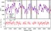 |
Fig. 1 Least-squares RV fit for RV with CARMENES VIS data for GJ 1265. Top: one observation (red) and the best fit model (blue) are shown. Data points within telluric regions (grey area) are a priori excluded. Data points classified as outliers are indicated in cyan. Bottom: fit residuals are shown. |
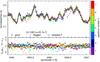 |
Fig. 2 Spectra coadding of seven CARMENES VIS spectra of GJ 1265. The seven observations (colour coded), each normalised by a background polynomial, are fitted by a uniform cubic B-spline (black) where basically each knot value is a free parameter (black dots). Points affected by tellurics or outlying by 5σ are excluded from the fit (open circles). |
The χ2(v) function sampled at  is explored for its global minimum. Around its minimum, the χ2 function takes a parabolic shape and the first derivative vanishes, (χ2)′ = 0. The Taylor expansion of the χ2 function at the minimum to second order is
  (9)Since we use cubic interpolation for the template, the second derivative of the template F (and of χ2) is continuous. Then a parabolic interpolation through the minimum of the χ2(v) function and the two adjacent neighbours provides a refined estimate for v and an error estimate for v can be obtained from the parabola curvature. The parabola minimum is located at the point,
 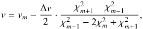 (10)where m indexes the discrete global minimum of
  (see Eq. (10.2.1) in Press et al. 1992, that is specialised here for a uniform grid, Δv = vk−vk−1, or Eq. (A.3)).
The uncertainty of v is estimated from Eq. (9) with the  criterion along with the curvature from Eq. (A.4)
  (11)This value might be rescaled with
  to account for under- or overdispersion of the fit.
Finally, a statistical analysis of the fit is performed. The χ2 and are computed. Linear residuals ri = fi−fmod,i exceeding the threshold  (12)where the clipping value κ is typically 3...5, are flagged as outliers (e.g. by setting their weights to zero wi = 0) and excluded in a repeated fitting. The same can be formulated with normalised residuals
 (13)Figure 1 illustrates the best fit between one observation and a template.
Each order is fitted separately and finally a weighted mean for the radial velocities vo from Eq. (10) with errors ϵvo from Eq. (11) over all orders o is computed (see also Fig. 3)  (14)with the error estimate
  (15)where wrms is the weighted root mean square and No is the number of orders.
2.3. Spectra coadding
At first glance, coadding spectra seems straightforward. However, the stellar spectra are Doppler shifted by potential Keplerian orbits and by the barycentric motion of Earth. Thus, spectra from different epochs are sampled at different wavelength footpoints. Hence naive coadding would require either some kind of resampling or interpolation of the observations onto a common wavelength grid (e.g. Anglada-Escudé & Butler 2012), which leads to difficulties in applying the data uncertainties, or calculating some form of bin means, which ignores the local gradient over the bin width. We point out that bin means are zeroth-order B-splines.
We carry out the “co-adding” with a uniform cubic basic spline (B-spline) regression to the normalised data. We emphasise here the term regression, which means least-squares fit and should be distinguished from spline interpolation and smoothing splines. There are several benefits of this approach: (1) B-spline regression is a linear least-squares method, and, therefore, it is fast; (2) there is no need to interpolate the data; (3) data point uncertainties can be easily taken into account; (4) robust statistics for outlier detections can be obtained with kappa-sigma clipping; and (5) a spline function is a direct outcome and consistent with our input for the forward model.
Given vn for the N observations from Sect. 2.2, we recompute the polynomials pn,i for each order (now with the mean RV vn) to normalise the data ( ) and calculate the Doppler-shifted wavelengths with Eq. (5). We factor
  in Eq. (3) and write it in the form
 ![\begin{equation} \chi^{2}=\sum_{n,i}p_{n,i}^{2}w_{n,i}\left[\frac{f_{n,i}}{p_{n,i}}-F(\lambda'_{n,i},b)\right]^{2}.\label{eq:chi2_template} \end{equation}](/articles/aa/full_html/2018/01/aa31483-17/aa31483-17-eq81.png) (16)Now the task is to find all the coefficients bk of the spline with K knots, so that the residuals are minimal. The knots of the template are positioned in a uniform grid in (logarithmic) wavelengths λk (lnλk) and fk (or B-spline coefficient bk, respectively). By default, the number of knots K is similar to the number of data points per spectrum in the order, i.e. we have about one knot per pixel. Depending on the needs, the sampling could also be decreased to obtain a smoother template (e.g. noisy observations or fast rotators) or increased to obtain subpixel sampling (many observations). It can be inferred from Eq. (16) that the normalised error estimates are
(16)Now the task is to find all the coefficients bk of the spline with K knots, so that the residuals are minimal. The knots of the template are positioned in a uniform grid in (logarithmic) wavelengths λk (lnλk) and fk (or B-spline coefficient bk, respectively). By default, the number of knots K is similar to the number of data points per spectrum in the order, i.e. we have about one knot per pixel. Depending on the needs, the sampling could also be decreased to obtain a smoother template (e.g. noisy observations or fast rotators) or increased to obtain subpixel sampling (many observations). It can be inferred from Eq. (16) that the normalised error estimates are  .
.
Equation (16) is a linear least-squares problem due to the linearity of the coefficients in the B-spline (de Boor 1978; Dierckx 1993; Eilers & Marx 1996) used to describe the template  (17)where B are the basic functions. Figure 2 shows the normalised and Doppler-shifted data and the best spline fit.
However, caution is needed when there are large gaps in the data, i.e. regions where we have no information to say anything about the template (i.e. no constraints for bk). Possible solutions are (1) splitting the spline fit at those points; (2) fitting penalised splines; or (3) heavily down-weight, but not fully reject, the flagged data points (outliers, tellurics), which caused the gaps. We chose the last option (down-weighting) for tellurics. This means that we include regions heavily contaminated by telluric lines in coadding, while in RV measurements they are totally excluded.
For each knot we estimate an error for the knot value as well as the number of contributing good points. We calculate the errors in the knot values by first estimating the error in the B-spline coefficients as  (18)and then through error propagation
  (19)This simplified estimate does not use the covariance matrix, since calculating the inverse matrix would be very time consuming.
To increase the robustness against outliers, a few (≤3) kappa-sigma clipping iterations (κ = 5) are performed for the coadding (similar as in Eq. (13)).
Problems can arise with this coadding method when the pixel phase coverage is small because of a small barycentric range owing to close observations or high ecliptic latitude. Such small coverage may lead to ringing in the spline function. Reverting to simple bin means (zeroth order B-splines) or using penalised splines (p-splines, as a generalisation of B-splines; Eilers & Marx 1996) may help in such situations. Also sharp (undersampled) features, such as cosmics and emission lines, may lead to ringing features. The SERVAL code offers the option to use p-splines, but the choice for the value of penalty/smoothing parameter in each particular case will require some user testing or cross-validation algorithms. We also point out the Gaussian process approach of Czekala et al. (2017), where the variance/smoothness parameter is a hyperparameter, and that B-splines and p-splines can be considered as a special case of Gaussian processes (Rasmussen & Williams 2006).
SERVAL also offers the possibility to use external templates, e.g. from other observed stars of similar spectral type or synthetic spectra. The latter may be useful to derive absolute RVs and line indices (Sect. 3.3).
3. Spectral diagnostic and activity indicators
3.1. Chromatic RV index
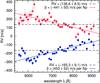 |
Fig. 3 Radial velocities measured in 42 orders of two CARMENES VIS observations of YZ CMi along with the simple weighted average (dashed black line) and the chromatic index (solid blue and red line). The wavelength axis is logarithmic. |
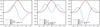 |
Fig. 4 Two Gaussian functions (solid black and dashed red) with slightly different shifts (left panel) and slightly different widths with same amplitude (middle panel) and same unit area (right panel). Their scaled difference (dotted green) is related to the first and/or second derivative (dash-dotted blue). |
In Eq. (14) we compute a simple weighted average for the RV over the orders. However, since the echelle orders are related to wavelength, we can also try to get some information about wavelength dependency for instance by simply extending the model to a straight line 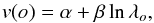 (20)where λo is a representative wavelength of echelle order o (e.g. lnλo = ⟨lnλo,i⟩). Via a χ2-fit we obtain a best fit estimate for the slope parameter β, which we call chromatic index. Its unit is velocity per wavelength ratio e (Neper, symbol Np). Figure 3 illustrates the slope definition for two observations of the active M dwarf YZ CMi.
The parameter α is considered as a nuisance parameter. Using the mean velocity v from Eq. (14) and the substitution α = v−βlnλv, we can re-parametrise Eq. (20) as 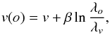 (21)where λv is the wavelength at which the slope intersects the weighted mean RV. This allows us to report an effective wavelength, which is in particular useful when comparing data from instruments covering different wavelengths.
In the definition of the chromatic index in Eq. (20), we chose lnλ, the natural logarithm of wavelength λ, as independent variable. While other choices like wavelength λ or order o, which is basically equivalent to reciprocal wavelength λ-1 (i.e. frequency), lead to qualitatively very similar results for β, our choice gives the same weights to each velocity element (resolution element) and is also useful when comparing data from a variety of instruments. Moreover, the wavelength range of 1 Np is typically covered by high resolution echelle spectrographs, i.e. the values of the slopes are of the order of the RV change over all echelle orders.
3.2. Differential line width (dLW)
A feature of the CCF method is that the CCF can be interpreted as a mean stellar line profile that is actually convolved with a kind of kernel. By analysing the CCF shape, for example by fitting a Gaussian function, we can obtain information about the moments, among them the centre of the Gaussian (first moment, i.e. RV) and the width (second moment, i.e. full width half maximum, FWHM). To obtain information about asymmetries (third moment, skewness), often bisectors are used (e.g. Figueira et al. 2013).
We study if there is an analogous set of parameters that can be associated with least-squares fitting. Since the CCF is basically a χ2 function, one could consider fitting a Gaussian function to the χ2 function. However, we argue that the shape (curvature, asymmetry) of the χ2 function is formed by the signal-to-noise of the observation, masking of outliers and tellurics, and also the simultaneous fit of the background polynomial.
In the following, we suggest another approach. We review a simple method to measure differential RVs as implied in Bouchy et al. (2001). Figure 4 (left) shows that when a Gaussian function is slightly displaced, the residuals, i.e. the difference between both curves, are correlated with the first derivative of the Gaussian function. In fact, this is actually the definition of the first derivative. From the scaling factor, which was already applied in Fig. 4, we can derive the RV 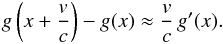 Now we replace on the left side the function difference by the residuals ri between (drifted) data and (flux-scaled) template, and on the right side the derivative of the Gaussian function by the derivative of the template. The derivative must be with respect to velocity, i.e.
  . The relation becomes
  (22)In simple terms, we scale the first derivative to the residuals. The best scaling factor v can be derived with a linear least-squares fit weighted with flux uncertainties σi. In Sect. 2.2, on the other hand, the RV shift was already applied by actually minimizing this correlation.
Now the question is whether we can find a similar relation using the first or higher derivatives to check for variations in the line width. Therefore, we vary the line width of the Gaussian. In one variant we keep the line height constant (Fig. 4, middle) and in another variant we keep the same area under the curve (Fig. 4, right). For both cases we plot again the scaled residuals and compare these residuals with squared first derivative (middle) and second derivative (right), respectively.
The case of unit area (right panel) results in balanced positive and negative deviations, which is more similar to the situation we are facing after a least-squares fit of the RV (Sect. 2.2). Indeed, we prove in Appendix B that the mean value of the second derivative is zero (the same is true for least-squares fit residuals) and that  (23)This relation is in a strict sense valid only for Gaussian functions, but it suggests simply scaling the second derivative of the template (
 ) to the residuals
  (24)Hence we have to assume that the stellar lines are Gaussian-like shaped. The relation also holds when we build up a spectrum by adding Gaussian lines at other positions and with different strengths due to the linearity. Then this also implies that it is applicable to blended lines. However, the lines should have all the same width. We point out that similar assumptions are made when fitting a Gaussian profile to the CCF.
The scaling factor Δσ carries information about line width changes and we compute its value via a weighted linear least-squares fit resulting in  (25)and estimate its uncertainty through error propagation as
  (26)The dLW is computed in each order and finally averaged similar to the RVs in Eqs. (14) and (15). The SERVAL programme propagates the uncertainties of the spectra which are mostly photon and readout noise. On top of this there can be other noise sources from the instrument, such as focus or resolution change, or observation, such as line broading due to barycentric motion during the exposure. Therefore, even quiet stars with presumable stable intrisic line shapes may show excess variations in line width indicators.
Since our template is a cubic B-spline, we can easily calculate the second derivative f′′ at each position of the spectrum. Also the third derivative would be possible and the possibility of defining a differential alternative to the bisector span in the CCF would appear very straightforward, but this is not yet implemented. Of course, the uncertainty in the higher order moments increase.
Owing to our differential approach, our width indicator σΔσ has also a differential nature, and, therefore, we call it differential line width (dLW). Its unit is m2/ s2 if the derivative is calculated in velocity or logarithmic wavelength scale. In analogy to differential RVs, in which an additive offset remains with respect to to absolute RVs, the offset now becomes multiplicative in the differential width (second moment). The σΔσ indicator is sensitive to regions where the second derivative is large, such as the cores of spectral lines (cf. Fig. 4, right panel).
Variations in the spectral line width can be intrinsic to the star, for example pulsation or activity, or of instrumental origin in the form of focus change and smearing due to the barycentric motion during exposure. In any case, correlation of a RV signal with line width variations would argue against a planet hypothesis.
3.3. Line indices
The SERVAL code also provides indices in the form of time series data for a number of spectral lines (e.g. Ca ii H&K, Hα, Na i D, and Ca ii IRT). Before measuring the line indices, we need to find the line positions, i.e. the absolute RVs. These can be obtained by measuring the RV of one spectrum against an absolute reference (e.g. a PHOENIX spectrum).
Following Kürster et al. (2003), the indices are computed as  (27)where ⟨f0⟩ is the mean flux around the line centre and ⟨f1⟩ and ⟨f2⟩ are the mean fluxes over reference regions.
As an example, we choose for Hα (λair = 6562.8 Å) the region [−40, +40] km s-1 and as reference [−300, −100] km s-1 and [+100,+300] km s-1. We apply a larger core region compared to Kürster et al. (2003), who only applied it to the inactive star GJ 699, to collect all Hα emission for most of the M dwarfs, while for most active stars an even wider range could be considered at the cost of decreasing index precision.
We estimate the error in the mean fluxes using the data error ϵi (28)This choice is not unique, but it preserves some information about the signal-to-noise ratio in the spectrum; in case of pure photon noise
  , it satisfies
  . From the stand point of least squares, the standard error of the mean would be calculated via the standard deviation as
  and for a weighted mean as
  (cf. Eq. (15)). However, when modelling a line such as Hα with a mean, i.e. we fit a box, we should be aware of a large model mismatch with this simplistic model making those error estimates misleading. Indeed, one could consider more tailored models, for example the Mount Wilson S-index employs a triangular shape (Duncan et al. 1991).
Finally, we simply propagate the errors from Eq. (28) through Eq. (27) to an uncertainty for the line index  (29)Sometimes (pseudo-) equivalent widths (pEW) are preferred instead of line indices. We outlined in Zechmeister et al. (2009) that pEWs are closely related to line indices, which might be interpreted as “pseudo line heights”. Indeed, both quantities measure the zero moment (area, integrated flux) and condense it into one parameter. This simple estimate is sufficient for studies on the activity level of stars and temporal variations. However, the true line shape is more complex (e.g. self-absorption features) and needs to be described by more moments/parameters.
We have also implemented a differential version for spectral line indices where the mean fluxes in Eq. (27) are replaced by the scaling factor between the observation and the coadded template. This method aims for optimal weights and highest precision and would be also applicable in case of missing data points, for example due to cosmics or tellurics, but we recommend this only for inactive stars.
4. Results
In this section we evaluate the performance of SERVAL using its RV precision, the dLW, and the chromatic index. To achieve this, we use data from HARPS and CARMENES. The HARPS instrument and its data reduction software has demonstrated long-term 1 m/s precision since its installation in 2003 (Mayor et al. 2003). Each of the points to be tested are evaluated for (1) a stable and inactive M dwarf (Barnard’s star), (2) a G4 dwarf with strong correlations between FWHM and RVs (ζ1 Ret), and (3) two very active M dwarfs (YZ CMi and GJ 3379). The time-series measurements are shown in Figs. 5−8.
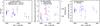 |
Fig. 5 Radial velocity (left), line width (middle), and chromatic index (right) time series for HARPS data of GJ 699. SERVAL results are indicated in blue solid diamonds and DRS in red open diamonds. |
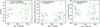 |
Fig. 7 Radial velocity (left), dLW (middle), and chromatic index (right) time series for CARMENES data of YZ CMi. |
4.1. Targets
GJ699.
Barnard’s star is an inactive M4V star. For comparison we use the same 22 HARPS observations as previously used in Anglada-Escudé & Butler (2012). The spectra were obtained between 2007-04-04 and 2008-05-02. All spectra were secured without simultaneous drift measurements and two spectra 4 were taken during twilight.
ζ1 Ret.
This G4 dwarf was found by Zechmeister et al. (2013) to have a strong correlation between RV and FWHM and hence we selected it as an example for dLW analysis. We analysed 61 HARPS measurements taken during 24 nights over a time span of 1401 days. Typical FWHM values of 7.1 km s-1 indicate that the star is not a slow rotator.
YZ CMi.
This star (GJ 285, Karmn J07446+035) is a very active M4.5 dwarf with significant rotation measured in several works (vsini ~ 5 km s-1, log (LHα/Lbol) = −3.48; Reiners et al. 2012; Jeffers et al. 2017), a photometric period of 2.78 d (West et al. 2015), an average magnetic field of the order of 3–4 kG, and local field strengths up to 7 kG (Shulyak et al. 2014). We obtained 45 CARMENES VIS observations spanning 480 days (from 2016-01-08 to 2017-05-01).
GJ 3379.
This star (G 099-049, Karmn J06000+027) is an active M4.0 dwarf with significant rotational broadening (vsini = (7.4 ± 0.8) km s-1, Delfosse et al. 1998). We found 16 HARPS spectra in the ESO archive and obtained 14 spectra with CARMENES for GJ 3379. We only used this star to compare the chromatic index between HARPS and CARMENES wavelength ranges.
4.2. Criterion 1: Radial velocity precision
GJ 699.
Figure 5 (left) compares the RVs derived with SERVAL (rms = 1.30 m/s) and the HARPS DRS pipeline (rms = 1.54 m/s), while Anglada-Escudé & Butler (2012) reported a dispersion of rms = 1.24 m/s for the same dataset. Secular acceleration is subtracted in all cases. This demonstrates the capability of SERVAL to achieve precise RVs at the 1 m/s level.
ζ1 Ret.
The RVs have an rms of 10 m/s (Fig. 6). Since there is activity-induced jitter, we cannot evaluate the individual RV performance with this star. Still, the RV difference between SERVAL and DRS CCF has an rms of 1.2 m/s and points to 1 m/s performance of SERVAL for solar-like stars as well.
YZ CMi.
The RVs show an rms of 85 m/s (Fig. 7, left). The variation takes place on short time scales (days) with a significant periodicity of 2.776 d with an amplitude of 120 m/s (Fig. 9 and a less significant one-day alias at 1.556 d and 100 m/s). This period also appears in the Hα-line equivalent width but at low significance.
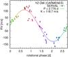 |
Fig. 9 Radial velocities of YZ CMi phase folded to a period of 2.776 d. The rotational phase is colour coded in reference to Fig. 12; blue and red correspond to the phases of predicted maximum blue shift and red shift, respectively. |
4.3. Criterion 2: dLW
GJ 699.
The comparison between dLW and FWHM, drawn on the left and right axes, respectively, is shown as a time series in the middle panel of Fig. 5. Both indicators have relatively similar error bars and vary significantly; we adopted ϵFWHM = 2.35ϵRV. Using the relation FWHM = 2.35σ for a Gaussian, we would expect  . This theoretical prediction is shown as a blue line in Fig. 10 (top left panel). We see that dLW values scatter around this prediction, but the large uncertainty for the best fitting slope shows that the dLW and FWHM correlate poorly for GJ 699. Surprisingly, we find a much better correlation of dLW with FWHM divided by the contrast indicator, which is the relative amplitude of the Gaussian fit (Fig. 10, top right). This is currently not well understood, but it likely reminds us that dLW and FWHM are not fully tracking the same effect. Indeed, the dLW indicator assumes that the area of the Gaussian-shaped line, i.e. the product of FWHM and contrast, remains constant, while a Gaussian fit to the CCF decomposes both parameters simultaneously. Hence, we could argue that additional contrast variations (on top of contrast ∝ FWHM-1) could lead to biased dLW measurements. Those contrast variations could be induced by imperfect background subtraction or have stellar origin, albeit we believe the latter is less likely for this quiet star. Alternatively, the poor dLW-FWHM correlation for GJ699 could point to a bias when fitting a Gaussian function to the CCF of an M dwarf, which is known to exhibit prominent side lobes (see e.g. Fig. 7 in Berdiñas et al. 2017). Neither dLW nor FWHM correlate with RVs.
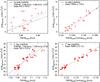 |
Fig. 10 Left: correlation between the DRS-FWHM and the SERVAL-dLW with HARPS data for the stars GJ 699 (top) and ζ1 Ret (bottom). The solid black line indicates the best fitting linear trend; the blue dashed line represents the theoretical prediction. Right: same as left panels, but the FWHM is divided by the contrast. |
ζ1 Ret.
The time series of dLW and FWHM already indicates a similar behaviour (Fig. 6, middle). Both, FWHM and dLW, correlate with RV (Fig. 11). There is also a direct correlation between dLW and FWHM; still the correlation improves again when dividing the FWHM by the contrast (Fig. 10, bottom panels).
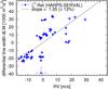 |
Fig. 11 Correlation between RV and dLW for HARPS data of ζ1 Ret. |
YZ CMi.
The dLW (Fig. 7, middle) reveals a 2.776 d period that we have already found in the RVs. The correlation between dLW and RV is not linear (Fig. 12, bottom and top), but we find that our observations follow a well-defined path when we colour code the rotational phase with this period. The one dLW outlier is an observation with an Hα flare. The spectrum has the highest Hα core emission and noticable rising Hα wings compared to the other spectra. Likely, the flare adds continuum flux over the full spectrum, leading primarily to line contrast variations. The flare event is not noticable in RV and chromatic index, although the point has maximum RV and minimum chromatic index.
4.4. Criterion 3: chromatic RV Index
GJ 699.
The chromatic index (Fig. 5, right) does not vary significantly. This is expected for an inactive and slowly rotating star.
ζ1 Ret.
The chromatic index (Fig. 6) shows long-term variations that seem to be anti-correlated with the RV long-term variations, which could be an activity cycle. However, the chromatic index does not follow the short-term variations of RV and dLW. Therefore, the chromatic index apparently has a complementary role to line width indicators.
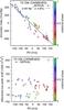 |
Fig. 12 Top: chromaticity (correlation between RV and chromatic index) for 45 CARMENES VIS spectra of YZ CMi. The left-most (RV = 165.3 m/s, β = 453 m/s/Np) and right-most data points (RV = 136.6 m/s, β = −441 m/s/Np) are the values derived in Fig. 3. Bottom: RV-dLW correlation is shown. |
YZ CMi.
In the top panel of Fig. 12, we show the chromatic index as a function of RV for our CARMENES observations of YZ CMi; both parameters are clearly anti-correlated. We call this correlation and the corresponding slope chromaticity κ. RV variations of ± 150 m/s correspond to variations of the chromatic index of ∓ 450 m/s/Np. Of course, due to the anti-correlation, the periodograms for chromatic index and RV have a similar shape and the 2.776 d period is also found in the chromatic index. For this period, we colour code our data in Fig. 12 according to their rotational phase. One can clearly follow how the individual observations are distributed throughout the rotational phase of YZ CMi.
The chromatic index-RV correlation demonstrates that the dominating effect in the RV variations of YZ CMi is wavelength dependent, which is consistent with the hypothesis that they are caused by co-rotating features such as active regions on the surface of the star. The wavelength-dependent temperature contrast between quiet and active regions is expected to cause a variation of the RVs as a function of wavelength (e.g. Fig. 12 in Reiners et al. 2010). Active regions (or spots) that are somewhat cooler (or hotter) than the photosphere show less contrast to the photosphere at longer wavelengths. The chromatic index attempts to capture this dependence on wavelength. The advantage of the chromatic index over chromospheric emission (Ca ii H&K, Hα) is that it comes with a directional sense, i.e. it can be positive and negative. The chromatic index is directly connected to RV because it is calculated from the same line profile deformation.
A negative chromaticity, as in case of YZ CMi, means that the RV scatter decreases towards redder wavelength. This amplitude decrease can been seen in Fig. 3 and is predicted with spot simulations (Desort et al. 2007; Reiners et al. 2010). The slope in the correlation plot (Fig. 12, top) provides information about spot temperatures. Moreover, we identify a separation between the values of the chromatic index at rotational phases 0.5 and 1, which would not be the case if the relation was simply linear and is probably related to convective blue shift. A deeper interpretation of these effects requires more detailed observations and goes beyond the scope of this paper.
Using the example of YZ CMi, we demonstrated that the chromatic index in the wavelength range of CARMENES VIS (550–970 nm) is a powerful tool for understanding RV variations induced by stellar activity. A closer look at the individual RVs per wavelength (Fig. 3) shows that a fairly tight relation between RV and wavelength exists for the wavelength range 600–920 nm, but the five spectral orders short of λ = 590 nm fail to follow this trend. We observe this behaviour in the other exposures of YZ CMi, too. The significance of this effect for YZ CMi and other stars needs more detailed investigation. There are two plausible explanations for the lack of correlation at shorter wavelengths: first, the contrast grows too high in that active regions no longer contribute to the observed spectrum in a significant way; and second that the intensity of spectral features at short wavelengths also differs dramatically between active and quiet regions (Reiners et al. 2010).
A possible way to investigate whether the chromatic index effect continues down to shorter wavelengths is to determine RVs for individual spectral orders of spectra taken with HARPS. This was attempted for the active M4.5 dwarf AD Leo by Reiners et al. (2013, Fig. 9). Interestingly, the activity-induced RV amplitude reported there grows with wavelength (positive chromaticity κ), but the effect is more than an order of magnitude weaker than what we observe in the CARMENES data of YZ CMi. Additionally, the two RV amplitudes shown for AD Leo by Reiners et al. (2013) that overlap with the CARMENES wavelength range in fact show a much steeper wavelength dependence with the same negative sign as observed in the CARMENES data for YZ CMi. The comparison between AD Leo and YZ CMi, however, remains inconclusive because we might just be seeing very different effects in different stars.
In order to make a more useful comparison of the HARPS and CARMENES wavelength ranges, we looked for targets that were observed with both instruments, albeit not simultaneously. One of the few targets available for this exercise is GJ 3379. Radial velocities and line indicators are shown in Fig. 8. The datasets were taken at very different times. The RVs from HARPS spectra exhibit an rms of 74 m/s while the CARMENES RVs show an rms of 21 m/s. The intrinsic uncertainties of the individual RV measurements are of the order of a few m/s in both cases and negligible for this comparison.
We calculated the chromatic index in both datasets and show the correlations between chromatic index and RV in Fig. 13. For our CARMENES data, chromatic index and RVs are correlated. The relation can be described by a linear fit with a gradient of −2.6 Np-1(± 21%). In the HARPS data, we find no correlation between chromatic index and RV, although the scatter in RV is higher than in the CARMENES data.
This comparison seems to indicate that the RVs of GJ 3379 show larger scatter at bluer wavelengths and that the RV variations at longer wavelengths are correlated with the chromatic index, while those at bluer wavelengths are not. However, an alternative explanation is that the RV jitter of the star changed during the course of a potential activity cycle; the HARPS and CARMENES data are separated in time by four years. One way to test this scenario is to compare RVs from the same wavelength range in both datasets; HARPS and CARMENES overlap in the range 550–690 nm. Unfortunately, this wavelength range is too short to draw definite conclusions about the chromatic index, and we have already shown above that the slope is most useful at longer wavelengths. Nevertheless, we find a correlation slope between chromatic index and RV of about −1 Np-1. Although the scatter around this relation is relatively high, HARPS and CARMENES data points are consistent with each other. The correlation between chromatic index and RVs is much weaker than for the full CARMENES wavelength range and the correlation itself is marginally significant. On the other hand, the RVs calculated from the limited wavelength range are precise enough to compare the two time series; in this case we find that the rms of CARMENES RVs (30 m/s) is significantly lower than the HARPS rms (77 m/s). It is unlikely that this effect is caused by differences between the two instruments because for both we estimate the internal uncertainties to be much smaller and comparable with each other (4 m/s). Thus, for now the case remains undecided. We find that GJ 3379 shows reduced activity jitter during the epoch observed with CARMENES, while the RV rms was high when it was observed with HARPS. Nevertheless, the CARMENES RVs show a correlation with chromatic index when the full CARMENES wavelength range is taken into account. We expect that such a correlation would still be visible when GJ 3379 exhibits larger RV variations, but simultaneous observations of the HARPS and CARMENES wavelength ranges are required to settle this question.
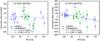 |
Fig. 13 Radial velocity-chromatic index correlation for GJ 3379. The fitted slope is the chromaticity of GJ 3379 in HARPS data (blue diamonds) and CARMENES data (green circles) using their full spectral range (left) and only the overlapping spectral region (right). |
5. Summary
We have presented our concept to derive high-precision RVs and have provided details on the creation of a template. Following an iterative and sequential approach we first derive approximate RVs measured against an observed spectrum and then improve the template by co-adding all observed spectra and recompute the RVs. The spectra are “coadded” via a weighted least-squares regression with a cubic B-spline.
The SERVAL code yields an output consisting of time series for high-precision RVs and a number of spectral indicators useful for further diagnostics as well as the high signal-to-noise templates partly cleaned from telluric contamination taking advantage of barycentric shifts. We find a similar performance when comparing the RV results from SERVAL and the HARPS-DRS pipeline using data for GJ 699 and ζ1 Ret. An additional example can also be found in Zechmeister et al. (2014), where an older version of SERVAL was applied to ~150 τ Cet spectra obtained during one night. This demonstrates that SERVAL produces RVs at a 1 m/s precision level.
Furthermore, we motivated a definition to study differential changes in the spectral line widths. We scale the second derivative of the template to the residuals from the fit for the best RVs and have shown that it can be useful in practice. This differential indicator nicely fits in our self-consistent framework of least-squares fitting (for differential RVs) without the need for external templates. Of course, this comes at the price that the differential results have no external accuracy, i.e. the line width remains unknown. In contrast, unbiased and accurate line width measurements for M dwarf spectra with their overall blended lines can be obtained with least-squares deconvolution (Barnes et al. 2012), but those are more complicated algorithms that require accurate line positions as input.
The chromatic index, while very simple in its definition, turns out to be a very powerful indicator to identify stellar activity in RV signals. We have shown that it correlates very well with RVs for the active M dwarf YZ CMi. Hence it will help us to identify signals that are associated with the intrinsic stellar variations rather than variations induced by Keplerian motion, to lower the detection limit for active and inactive stars because it can be used to remove and disentangle the activity contribution from the RVs, and to better understand the physics of the stars, such as spot temperature or convective blue shift. The chromatic index summarises in one value a first-order effect of wavelength dependence in the RVs and is well suited for an efficient analysis. Still, a more detailed investigation in smaller wavelength ranges might further our understanding of the wavelength dependence of stellar radial velocities (Reiners et al. 2013; Feng et al. 2017). A large wavelength range, such as that offered by CARMENES, is essential for this.
This requires internet access (http://astroutils.astronomy.ohio-state.edu/exofast/barycorr.html) or an installation of IDL.
Acknowledgments
We thank J. Zhao, Y. Thiele, E. Nagel, L. Nortmann, and G. Anglada-Escudé for software testing and helpful discussions. M.Z. acknowledges support from the Deutsche Forschungsgemeinschaft under DFG RE 1664/12-1 and Research Unit FOR2544, project No. RE 1664/14-1. I.R. acknowledges support by the Spanish Ministry of Economy and Competitiveness (MINECO) and the Fondo Europeo de Desarrollo Regional (FEDER) through grant ESP2016-80435-C2-1-R, as well as the support of the Generalitat de Catalunya/CERCA programme. V. Wolthoff acknowledges funding from the DFG Research Unit FOR2544, project No. RE 2694/4-1. V.J.S.B. are supported by grant AYA2015-69350-C3-2-P from the Spanish Ministry of Economy and Competiveness (MINECO). The UCM, CAB, and IAA team members acknowledges support by the Spanish Ministry of Economy and Competitiveness (MINECO) from projects AYA2016-79425- C3-1,2,3-P. CARMENES is an instrument for the Centro Astronómico Hispano-Alemán de Calar Alto
(CAHA, Almería, Spain). CARMENES is funded by the German Max-Planck-Gesellschaft (MPG), the Spanish Consejo Superior de Investigaciones Científicas (CSIC), the European Union through FEDER/ERF funds, and the members of the CARMENES Consortium (Max-Planck-Institut für Astronomie, Instituto de Astrofísica de Andalucía, Landessternwarte Königstuhl, Institut de Ciències de l’Espai, Insitut für Astrophysik Göttingen, Universidad Complutense de Madrid, Thüringer Landessternwarte Tautenburg, Instituto de Astrofísica de Canarias, Hamburger Sternwarte, Centro de Astrobiología and Centro Astronómico Hispano-Alemán), with additional contributions by the Spanish Ministry of Economy, the German Science Foundation (DFG) through the Major Research Instrumentation Programme and DFG Research Unit FOR2544 “Blue Planets around Red Stars”, the Klaus Tschira Stiftung, the states of Baden-Württemberg and Niedersachsen, and by the Junta de Andalucía.
References
- Anglada-Escudé, G., & Butler, R. P. 2012, ApJS, 200, 15 [NASA ADS] [CrossRef] [Google Scholar]
- Astudillo-Defru, N., Bonfils, X., Delfosse, X., et al. 2015, A&A, 575, A119 [NASA ADS] [CrossRef] [EDP Sciences] [Google Scholar]
- Barnes, J. R., Jenkins, J. S., Jones, H. R. A., et al. 2012, MNRAS, 424, 591 [NASA ADS] [CrossRef] [Google Scholar]
- Berdiñas, Z. M., Rodríguez-López, C., Amado, P. J., et al. 2017, MNRAS, 469, 4268 [NASA ADS] [CrossRef] [Google Scholar]
- Bouchy, F., Pepe, F., & Queloz, D. 2001, A&A, 374, 733 [NASA ADS] [CrossRef] [EDP Sciences] [Google Scholar]
- Butler, R. P., Marcy, G. W., Williams, E., et al. 1996, PASP, 108, 500 [NASA ADS] [CrossRef] [Google Scholar]
- Caballero, J. A., Guàrdia, J., López del Fresno, M., et al. 2016, in Observatory Operations: Strategies, Processes, and Systems VI, Proc. SPIE, 9910, 99100E [Google Scholar]
- Chelli, A. 2000, A&A, 358, L59 [NASA ADS] [Google Scholar]
- Czekala, I., Mandel, K. S., Andrews, S. M., et al. 2017, ApJ, 840, 49 [NASA ADS] [CrossRef] [Google Scholar]
- David, M., Blomme, R., Frémat, Y., et al. 2014, A&A, 562, A97 [NASA ADS] [CrossRef] [EDP Sciences] [Google Scholar]
- de Boor, C. 1978, A practical guide to splines. (New York: Springer) [Google Scholar]
- Delfosse, X., Forveille, T., Perrier, C., & Mayor, M. 1998, A&A, 331, 581 [NASA ADS] [Google Scholar]
- Desort, M., Lagrange, A.-M., Galland, F., Udry, S., & Mayor, M. 2007, A&A, 473, 983 [NASA ADS] [CrossRef] [EDP Sciences] [Google Scholar]
- Dierckx, P. 1993, Curve and surface fitting with splines, Monographs on Numerical Analysis (Oxford: Clarendon) [Google Scholar]
- Duncan, D. K., Vaughan, A. H., Wilson, O. C., et al. 1991, ApJS, 76, 383 [NASA ADS] [CrossRef] [Google Scholar]
- Eilers, P. H. C., & Marx, B. D. 1996, Statist. Sci., 11, 89 [CrossRef] [Google Scholar]
- Endl, M., Kürster, M., & Els, S. 2000, A&A, 362, 585 [Google Scholar]
- Feng, F., Tuomi, M., & Jones, H. R. A. 2017, A&A, 605, A103 [NASA ADS] [CrossRef] [EDP Sciences] [Google Scholar]
- Figueira, P., Santos, N. C., Pepe, F., Lovis, C., & Nardetto, N. 2013, A&A, 557, A93 [NASA ADS] [CrossRef] [EDP Sciences] [Google Scholar]
- Hadrava, P. 2004, Publications of the Astronomical Institute of the Czechoslovak Academy of Sciences, 92, 15 [Google Scholar]
- Hensberge, H., & Pavlovski, K. 2007, in Binary Stars as Critical Tools & Tests in Contemporary Astrophysics, eds. W. I. Hartkopf, P. Harmanec, & E. F. Guinan, IAU Symp., 240, 136 [Google Scholar]
- Hrudková, M. 2009, Ph.D. Thesis, Charles University Prague [Google Scholar]
- Jeffers, S. V., Schoefer, P., Lamert, A., et al. 2017, A&A, accepted [Google Scholar]
- Kürster, M., Endl, M., Rouesnel, F., et al. 2003, A&A, 403, 1077 [NASA ADS] [CrossRef] [EDP Sciences] [Google Scholar]
- Mayor, M., Pepe, F., Queloz, D., et al. 2003, The Messenger, 114, 20 [NASA ADS] [Google Scholar]
- Pepe, F., Mayor, M., Galland, F., et al. 2002, A&A, 388, 632 [NASA ADS] [CrossRef] [EDP Sciences] [Google Scholar]
- Press, W. H., Teukolsky, S. A., Vetterling, W. T., & Flannery, B. P. 1992, Numerical recipes in C, The art of scientific computing (CUP) [Google Scholar]
- Queloz, D. 1995, in New Developments in Array Technology and Applications, eds. A. G. D. Philip, K. Janes, & A. R. Upgren, IAU Symp., 167, 221 [Google Scholar]
- Quirrenbach, A., Amado, P. J., Caballero, J. A., et al. 2016, in Ground-based and Airborne Instrumentation for Astronomy VI, Proc. SPIE, 9908, 990812 [Google Scholar]
- Rasmussen, C. E., & Williams, C. K. I. 2006, Gaussian Processes for Machine Learning, Adaptive Computation and Machine Learning (The MIT Press) [Google Scholar]
- Reiners, A., Bean, J. L., Huber, K. F., et al. 2010, ApJ, 710, 432 [NASA ADS] [CrossRef] [Google Scholar]
- Reiners, A., Joshi, N., & Goldman, B. 2012, AJ, 143, 93 [NASA ADS] [CrossRef] [Google Scholar]
- Reiners, A., Shulyak, D., Anglada-Escudé, G., et al. 2013, A&A, 552, A103 [NASA ADS] [CrossRef] [EDP Sciences] [Google Scholar]
- Shulyak, D., Reiners, A., Seemann, U., Kochukhov, O., & Piskunov, N. 2014, A&A, 563, A35 [NASA ADS] [CrossRef] [EDP Sciences] [Google Scholar]
- West, A. A., Weisenburger, K. L., Irwin, J., et al. 2015, ApJ, 812, 3 [NASA ADS] [CrossRef] [Google Scholar]
- Wright, J. T., & Eastman, J. D. 2014, PASP, 126, 838 [NASA ADS] [CrossRef] [EDP Sciences] [Google Scholar]
- Zechmeister, M., Kürster, M., & Endl, M. 2009, A&A, 505, 859 [NASA ADS] [CrossRef] [EDP Sciences] [Google Scholar]
- Zechmeister, M., Kürster, M., Endl, M., et al. 2013, A&A, 552, A78 [NASA ADS] [CrossRef] [EDP Sciences] [Google Scholar]
- Zechmeister, M., Anglada-Escudé, G., & Reiners, A. 2014, A&A, 561, A59 [NASA ADS] [CrossRef] [EDP Sciences] [Google Scholar]
- Zucker, S. 2003, MNRAS, 342, 1291 [Google Scholar]
Appendix A: Parabolic interpolation
We want to derive the interpolating parabola y = ax2 + bx + c through the three points (xi,yi), (xi−1,yi−1), and (xi + 1,yi + 1). The points should be equidistant, i.e. xi + 1 − xi = Δx and xi − xi−1 = Δx. Now we centre points to (xi,yi) and the three transformed points are (0,0), (− Δx,Y-1) and  . Inserting into the parabola equation leads to a system of three equations
 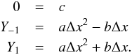 (A.1)The solution is
 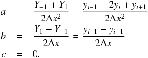 (A.2)Reforming the parabola equation to
 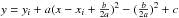 , the extremum of the parabola is at
 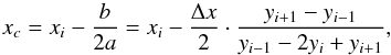 (A.3)and the second derivative at xc is
 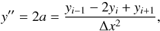 (A.4)which is the definition of the finite second derivative.
Appendix B: Derivatives of the Gaussian function
We start with a Gaussian function with unit amplitude. Their first and second derivatives (with respect to x) are given by 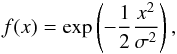 (B.1)
(B.1)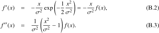 We seek to understand how the residuals should appear when we change the width while keeping the amplitude. The derivative of Eq. (B.1) with respect to parameter σ can be written as
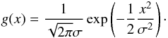
 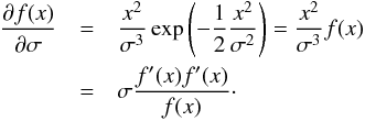 (B.4)When we are interested in the residuals while conserving the area under the curves (Fig. 4, right panel), we have to include the normalising factor
 (B.5)The relation of g′(x) and g′′(x) to g(x) is the same as for f(x). However, the derivative with respect to σ is
  (B.6)This suggests that we correlate the second derivative of the spectrum with the residuals when we want to infer differential variations in the width.
The mean value of the second derivative is  (B.7)
(B.7)
All Figures
|
Fig. 1 Least-squares RV fit for RV with CARMENES VIS data for GJ 1265. Top: one observation (red) and the best fit model (blue) are shown. Data points within telluric regions (grey area) are a priori excluded. Data points classified as outliers are indicated in cyan. Bottom: fit residuals are shown. |
| In the text | |
|
Fig. 2 Spectra coadding of seven CARMENES VIS spectra of GJ 1265. The seven observations (colour coded), each normalised by a background polynomial, are fitted by a uniform cubic B-spline (black) where basically each knot value is a free parameter (black dots). Points affected by tellurics or outlying by 5σ are excluded from the fit (open circles). |
| In the text | |
|
Fig. 3 Radial velocities measured in 42 orders of two CARMENES VIS observations of YZ CMi along with the simple weighted average (dashed black line) and the chromatic index (solid blue and red line). The wavelength axis is logarithmic. |
| In the text | |
|
Fig. 4 Two Gaussian functions (solid black and dashed red) with slightly different shifts (left panel) and slightly different widths with same amplitude (middle panel) and same unit area (right panel). Their scaled difference (dotted green) is related to the first and/or second derivative (dash-dotted blue). |
| In the text | |
|
Fig. 5 Radial velocity (left), line width (middle), and chromatic index (right) time series for HARPS data of GJ 699. SERVAL results are indicated in blue solid diamonds and DRS in red open diamonds. |
| In the text | |
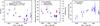 |
Fig. 6 Same as Fig. 5 but for ζ1 Ret. |
| In the text | |
|
Fig. 7 Radial velocity (left), dLW (middle), and chromatic index (right) time series for CARMENES data of YZ CMi. |
| In the text | |
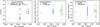 |
Fig. 8 Same as Fig. 7, but for GJ 3379 and HARPS (blue diamonds) and CARMENES (green circles) data. |
| In the text | |
|
Fig. 9 Radial velocities of YZ CMi phase folded to a period of 2.776 d. The rotational phase is colour coded in reference to Fig. 12; blue and red correspond to the phases of predicted maximum blue shift and red shift, respectively. |
| In the text | |
|
Fig. 10 Left: correlation between the DRS-FWHM and the SERVAL-dLW with HARPS data for the stars GJ 699 (top) and ζ1 Ret (bottom). The solid black line indicates the best fitting linear trend; the blue dashed line represents the theoretical prediction. Right: same as left panels, but the FWHM is divided by the contrast. |
| In the text | |
|
Fig. 11 Correlation between RV and dLW for HARPS data of ζ1 Ret. |
| In the text | |
|
Fig. 12 Top: chromaticity (correlation between RV and chromatic index) for 45 CARMENES VIS spectra of YZ CMi. The left-most (RV = 165.3 m/s, β = 453 m/s/Np) and right-most data points (RV = 136.6 m/s, β = −441 m/s/Np) are the values derived in Fig. 3. Bottom: RV-dLW correlation is shown. |
| In the text | |
|
Fig. 13 Radial velocity-chromatic index correlation for GJ 3379. The fitted slope is the chromaticity of GJ 3379 in HARPS data (blue diamonds) and CARMENES data (green circles) using their full spectral range (left) and only the overlapping spectral region (right). |
| In the text | |
Current usage metrics show cumulative count of Article Views (full-text article views including HTML views, PDF and ePub downloads, according to the available data) and Abstracts Views on Vision4Press platform.
Data correspond to usage on the plateform after 2015. The current usage metrics is available 48-96 hours after online publication and is updated daily on week days.
Initial download of the metrics may take a while.