© ESO, 2017

1. Introduction

Measurements of a quantity of interest can almost never be obtained without contributions of stochastic processes beyond our control. Examples of such processes in astronomy may be thermal noise from detectors and effects induced by variable atmospheric conditions in ground-based observations. In other cases, variability in the measured quantity itself such as stochastic light variations caused by stellar convection can be among these processes. Whether we consider this stochastic contribution noise or signal certainly depends on the adopted point of view.

In the analysis of data, the measurement uncertainty plays an important role. For instance, the application of χ² in tests of goodness of fit requires knowledge of the uncertainty in the individual measurements. If these cannot be accurately determined a priori as is often the case, the properties of the noise have to be estimated a posteriori from the data set itself.

While we may not have accurate knowledge about the actual distribution of the stochastic noise contribution, normally distributed errors are often a highly useful assumption, in particular, if only the general magnitude of the error is known or of interest (e.g., Jaynes 2003, Chap. 7). In many cases, including ours, the additional assumption of uncorrelated errors is made.

Of course, the problem of estimating the noise from the data is not new, and scientists have been using different approaches to obtain an estimate of the amplitude of the noise or the signal-to-noise ratio. Often, some fraction of the data set would be approximated using for example, a polynomial model via least-squares fitting so that, subsequently, the distribution of the residuals can be studied to estimate the amplitude of the noise term. While it remains immaterial whether the model is physically motivated or not, we usually lack detailed knowledge about both the noise and the signal. In highly variable data sets it may then be hard to identify even moderately extended sections, for which we may reasonably presume that they can be appropriately represented with a model such as a low-order polynomial to obtain the residuals. Furthermore, every such data set may need individual treatment in such an analysis. Therefore, techniques with better properties to handle such data are desirable.

To obtain reliable noise estimates from spectroscopic data, Stoehr et al. (2008) present the DER_SNR algorithm. Given a set of spectral bins, f_i, from which the noise contribution is to be estimated, Stoehr et al. (2008) propose the following three-step procedure: First, the median signal, med_i(f_i), is determined, where med_i indicates the median taken over the index i. Second, the standard deviation, σ, of the noise contribution is estimated from the expression 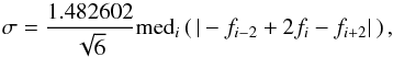$\mathit{\sigma }\mathrm{=}\frac{\mathrm{1.482602}}{\sqrt{\mathrm{6}}}{\mathrm{med}}_{\mathit{i}}\left(\hspace{0.17em}\mathrm{|}\mathrm{-}{\mathit{f}}_{\mathit{i}\mathrm{-}\mathrm{2}}\mathrm{+}\mathrm{2}{\mathit{f}}_{\mathit{i}}\mathrm{-}{\mathit{f}}_{\mathit{i}\mathrm{+}\mathrm{2}}\mathrm{|}\hspace{0.17em}\right)\mathit{,}$(1)where the factor of ≈1.48 corrects for bias (see Sect. 2.6). The sum in parenthesis is proportional to the second numerical derivative. For a sufficiently smooth and well-sampled signal, it vanishes except for noise contributions and, thus, becomes a measure for the noise. While Stoehr et al. (2008) found this form the optimal choice in their applications, they also point out that higher-order derivatives can be used. Third, the DER_SNR noise estimate is computed by dividing the median flux by the estimated noise.

In this paper, we take up the idea behind the DER_SNR algorithm, viz., to first obtain a set of numerical derivatives, which we call the β sample, from the data and derive the standard deviation, σ, of the noise contribution from it. In accordance with these steps, we refer to the more general concept of estimating the noise from numerical derivatives as the βσ procedure, which is identical to the DER_SNR algorithm for specific parameter settings (see Sect. 2.7). We explicitly treat the case of unevenly sampled data and study the statistical properties of the resulting noise estimates. Combining the latter with results obtained from synthetic and real data sets, we provide suggestions for the general application of the procedure.

2. The βσ procedure

We assume that we take measurements of some quantity Y, whose value depends on (at least) one other variable t, which may be a continuous or discrete parameter such as time or wavelength. Measurements of Y are taken at specific instances t_i, yielding data points (t_i,y_i), where y_i is the value of Y measured at t_i. We denote the number of data points by n_d.

We further assume that the behavior of Y is given by some (unknown) function g(t). The only restriction we impose on g(t) is that it may be possible to expand it into a Taylor series at any point, t₀, so that 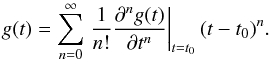$\mathit{g}\mathrm{\left(}\mathit{t}\mathrm{\right)}\mathrm{=}\sum _{\mathit{n}\mathrm{=}\mathrm{0}}^{\mathrm{\infty }}{\frac{\mathrm{1}}{\mathit{n}\mathrm{!}}\frac{{\mathit{\partial }}^{\mathit{n}}\mathit{g}\mathrm{\left(}\mathit{t}\mathrm{\right)}}{\mathit{\partial }{\mathit{t}}^{\mathit{n}}}|}_{\mathit{t}\mathrm{=}{\mathit{t}}_{\mathrm{0}}}\mathrm{(}\mathit{t}\mathrm{-}{\mathit{t}}_{\mathrm{0}}{\mathrm{)}}^{\mathit{n}}\mathit{.}$(2)It is sufficient that the expansion can be obtained up to a finite order, which will be specified later.

In addition to g(t), we allow for an additional stochastic contribution to the data points, which we indicate by ϵ_i. This contribution may, for example, be attributable to imperfections in the measurements process or a stochastic process contributing to the data. At any rate, our measurements will be composed of both terms, so that y_i = g(t_i) + ϵ_i. We assume the ϵ_i to be independent realizations of a Gaussian random variable with mean zero and (unknown) standard deviation σ₀. While any random process may produce this term, we will generally refer to it as noise contribution in the following. Given these assumptions, we now wish to estimate the magnitude of the noise term, σ₀, without specific knowledge about the underlying process giving rise to g(t).

2.1. Constant and slowly varying signals

To start, we assume that g(t) = c for any t with some constant c. In this case, we can be sure that the sample of data points, y_i, was drawn from a Gaussian distribution with standard deviation σ₀, and an estimate of the standard deviation in that sample would, thus, readily provide an estimate of the coveted amplitude of noise, σ₀.

Now we alleviate the constraints on g(t) and allow a slowly varying function, by which we mean that the difference between any two neighboring data points, y_{i + 1} and y_i, is expected to be dominated by the Gaussian random contribution, that is, g(t_{i + 1})−g(t_i) ≪ σ₀. Thus, we effectively postulate that g(t) can be approximated by a constant between any two neighboring data points¹. Even in the case of slow variation, however, we may still expect that the variation in the signal dominates the noise contribution on larger scales, that is, g(t_{i + q})−g(t_i) ≫ σ₀ for sufficiently large index offset q > 1. Consequently, the variation may be dominated by the actual signal, g(t), beyond the sampling scale, and we may no longer rely on the fact that the sample of data points is drawn from a Gaussian parent distribution with standard deviation σ₀. Thus, an estimate of the standard deviation in this sample may yield a value arbitrarily far off the true amplitude of the noise, σ₀. While this estimate would always be expected to be larger than σ₀ given that the g(t_i) and ϵ_i are uncorrelated, this fact helps little to mitigate the problem.

Facing this situation, we now construct a sample of values whose parent distribution is known and entirely determined by the noise; this set will be dubbed the β sample. In particular, we take advantage of the premise of slow variation. To obtain the β sample, we subdivide the sample of data points into subsets, each consisting of two consecutive data points. For instance, the first subset could comprise the data points y₀ and y₁, the second one the points y₂ and y₃, and so on. Of course different strategies for subdivisions are conceivable (see Sect. 2.5).

The idea now is to combine the data points in these subsets such that the influence of g(t) is minimized. Under our above assumptions, this is the case, if we subtract the values of neighboring data points. Therefore, we proceed by calculating a sample of differences, which we dub the α sample, for example, 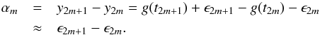$\begin{array}{ccc}{\mathit{\alpha }}_{\mathit{m}}& \mathrm{=}& {\mathit{y}}_{\mathrm{2}\mathit{m}\mathrm{+}\mathrm{1}}\mathrm{-}{\mathit{y}}_{\mathrm{2}\mathit{m}}\mathrm{=}\mathit{g}\mathrm{\left(}{\mathit{t}}_{\mathrm{2}\mathit{m}\mathrm{+}\mathrm{1}}\mathrm{\right)}\mathrm{+}{\mathit{ϵ}}_{\mathrm{2}\mathit{m}\mathrm{+}\mathrm{1}}\mathrm{-}\mathit{g}\mathrm{\left(}{\mathit{t}}_{\mathrm{2}\mathit{m}}\mathrm{\right)}\mathrm{-}{\mathit{ϵ}}_{\mathrm{2}\mathit{m}}\\ & \mathrm{\approx }& \end{array}$(3)Here and throughout this work, the index m is used to enumerate the subsets and subscript the quantities derived from the subsets of data points. As the ϵ_i are independent and drawn from a normal distribution, the α sample will also adhere to a Gaussian distribution with a standard deviation of $\sqrt{\mathrm{2}}{\mathit{\sigma }}_{\mathrm{0}}$ because the variances of the parent distributions of the noise terms add. Consequently, the sample of values ${\mathit{\beta }}_{\mathit{m}}\mathrm{=}\frac{{\mathit{\alpha }}_{\mathit{m}}}{\sqrt{\mathrm{2}}}\mathit{,}$(4)follows a normal distribution with standard deviation σ₀. An estimate of the standard deviation in this sample will yield an estimate of σ₀irrespective of g(t) as long as it varies slowly in the above sense.

The procedure used in Eq. (3) is essentially that of (first-order) differencing used in time series analyses to remove trends and produce a stationary time series (e.g., Shumway & Stoffer 2006). In those cases, where the local approximation of g(t) by a constant becomes insufficient, an approximation by a higher order polynomial can still lead to a properly distributed β sample.

2.2. Equidistant sampling

Let (t_k,y_k) with 0 ≤ k ≤ M be a subsample of M + 1 data points extracted from the original data set so that t_{k + 1}−t_k = Δt. In fact, data sets with equidistant sampling are not uncommon; examples in astronomy can be light curves or spectra.

If we expand g(t) around the point t₀ and stop the Taylor expansion at order N, g(t) is approximated by 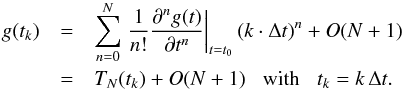$\begin{array}{ccc}\mathit{g}\mathrm{\left(}{\mathit{t}}_{\mathit{k}}\mathrm{\right)}& \mathrm{=}& \sum _{\mathit{n}\mathrm{=}\mathrm{0}}^{\mathit{N}}{\frac{\mathrm{1}}{\mathit{n}\mathrm{!}}\frac{{\mathit{\partial }}^{\mathit{n}}\mathit{g}\mathrm{\left(}\mathit{t}\mathrm{\right)}}{\mathit{\partial }{\mathit{t}}^{\mathit{n}}}|}_{\mathit{t}\mathrm{=}{\mathit{t}}_{\mathrm{0}}}\mathrm{(}\mathit{k}\mathrm{·}\mathrm{\Delta }\mathit{t}{\mathrm{)}}^{\mathit{n}}\mathrm{+}\mathit{O}\mathrm{(}\mathit{N}\mathrm{+}\mathrm{1}\mathrm{)}\\ & \mathrm{=}& {\mathit{T}}_{\mathit{N}}\mathrm{\left(}{\mathit{t}}_{\mathit{k}}\mathrm{\right)}\mathrm{+}\mathit{O}\mathrm{(}\mathit{N}\mathrm{+}\mathrm{1}\mathrm{)}\mathrm{with}{\mathit{t}}_{\mathit{k}}\mathrm{=}\mathit{k}\hspace{0.17em}\mathrm{\Delta }\mathit{t}\mathit{.}\end{array}$(5)Therefore, our data points can be approximated by the Nth-order polynomial approximation z_N,k = T_N(t_k) + ϵ_k ≈ y_k, and we dub N the “order of approximation”. If g(t) is a polynomial of degree ≤N, the equality is exact so that z_N,k = y_k.

We now wish to linearly combine M + 1 approximations, z_N,0...M, so that all polynomial contributions cancel, that is, 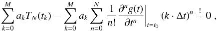$\sum _{\mathit{k}\mathrm{=}\mathrm{0}}^{\mathit{M}}{\mathit{a}}_{\mathit{k}}{\mathit{T}}_{\mathit{N}}\mathrm{\left(}{\mathit{t}}_{\mathit{k}}\mathrm{\right)}\mathrm{=}\sum _{\mathit{k}\mathrm{=}\mathrm{0}}^{\mathit{M}}{\mathit{a}}_{\mathit{k}}\sum _{\mathit{n}\mathrm{=}\mathrm{0}}^{\mathit{N}}{\frac{\mathrm{1}}{\mathit{n}\mathrm{!}}\frac{{\mathit{\partial }}^{\mathit{n}}\mathit{g}\mathrm{\left(}\mathit{t}\mathrm{\right)}}{\mathit{\partial }{\mathit{t}}^{\mathit{n}}}|}_{\mathit{t}\mathrm{=}{\mathit{t}}_{\mathrm{0}}}\mathrm{(}\mathit{k}\mathrm{·}\mathrm{\Delta }\mathit{t}{\mathrm{)}}^{\mathit{n}}\stackrel{\mathrm{!}}{\mathrm{=}}\mathrm{0}\mathit{,}$(6)where both the coefficients a_k and M are yet to be determined. As Eq. (6) is to hold for arbitrary Δt, it has to hold for all 0 ≤ n ≤ N separately. Combining constant terms into c_n, we obtain 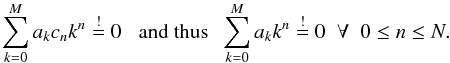$\sum _{\mathit{k}\mathrm{=}\mathrm{0}}^{\mathit{M}}{\mathit{a}}_{\mathit{k}}{\mathit{c}}_{\mathit{n}}{\mathit{k}}^{\mathit{n}}\stackrel{\mathrm{!}}{\mathrm{=}}\mathrm{0}\mathrm{andthus}\sum _{\mathit{k}\mathrm{=}\mathrm{0}}^{\mathit{M}}{\mathit{a}}_{\mathit{k}}{\mathit{k}}^{\mathit{n}}\stackrel{\mathrm{!}}{\mathrm{=}}\mathrm{0}\mathrm{\forall }\mathrm{0}\mathrm{\le }\mathit{n}\mathrm{\le }\mathit{N}\mathit{.}$(7)This expression holds for M = N + 1 and 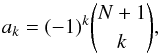${\mathit{a}}_{\mathit{k}}\mathrm{=}\mathrm{(}\mathrm{-}\mathrm{1}{\mathrm{)}}^{\mathit{k}}\left(\begin{array}{c}\mathit{N}\mathrm{+}\mathrm{1}\\ \mathit{k}\end{array}\right)\mathit{,}$(8)(e.g., Ruiz 1996, Corollary 2). Thus, the relation N + 2 = M + 1 between the order of approximation, N, and the required sample size of data points is established to make Eq. (6) hold. Along with the a_k, any multiple, γa_k, with γ ∈R also solves the equation. As this will prove irrelevant for our purpose, we set γ = 1.

From the above, we see that a set of N + 2 data point approximations of order N, z_N,k, can be combined to yield a weighted sum of noise terms 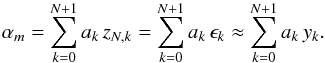${\mathit{\alpha }}_{\mathit{m}}\mathrm{=}\sum _{\mathit{k}\mathrm{=}\mathrm{0}}^{\mathit{N}\mathrm{+}\mathrm{1}}{\mathit{a}}_{\mathit{k}}\hspace{0.17em}{\mathit{z}}_{\mathit{N,k}}\mathrm{=}\sum _{\mathit{k}\mathrm{=}\mathrm{0}}^{\mathit{N}\mathrm{+}\mathrm{1}}{\mathit{a}}_{\mathit{k}}\hspace{0.17em}{\mathit{ϵ}}_{\mathit{k}}\mathrm{\approx }\sum _{\mathit{k}\mathrm{=}\mathrm{0}}^{\mathit{N}\mathrm{+}\mathrm{1}}{\mathit{a}}_{\mathit{k}}\hspace{0.17em}{\mathit{y}}_{\mathit{k}}\mathit{.}$(9)Again, m is an index, enumerating the subsets of data points from which the α_m are calculated (cf., Sect. 2.5). The last relation in Eq. (9) results from y_k ≈ z_N,k and shows that realizations of α can be obtained from measurements, y_k, given that the polynomial approximation is valid so that y_k−z_N,k ≪ σ₀.

In fact, the resulting expression corresponds to that obtained from N + 1 applications of differencing (Shumway & Stoffer 2006) and can be understood to be proportional to a numerical derivative of order N + 1 as obtained from the forward method of finite differences (e.g., Fornberg 1988). When applied to the Nth order polynomial approximation of g(t), the derivative of order N + 1 is necessarily zero.

As we assume identically distributed, independent Gaussian noise, also α_m follows a Gaussian distribution with a variance, ${\mathit{\sigma }}_{\mathit{\alpha ,m}}^{\mathrm{2}}$, of $\begin{array}{ccc}{\mathit{\sigma }}_{\mathit{\alpha ,m}}^{\mathrm{2}}\mathrm{=}{\mathit{\sigma }}_{\mathit{\alpha }}^{\mathrm{2}}& \mathrm{=}& \sum _{\mathit{k}\mathrm{=}\mathrm{0}}^{\mathit{N}\mathrm{+}\mathrm{1}}{\mathit{a}}_{\mathit{k}}^{\mathrm{2}}\hspace{0.17em}{\mathit{\sigma }}_{\mathrm{0}}^{\mathrm{2}}\mathrm{=}\sum _{\mathit{k}\mathrm{=}\mathrm{0}}^{\mathit{N}\mathrm{+}\mathrm{1}}{\left(\mathrm{(}\mathrm{-}\mathrm{1}{\mathrm{)}}^{\mathit{k}}\left(\begin{array}{c}\mathit{N}\mathrm{+}\mathrm{1}\\ \mathit{k}\end{array}\right)\right)}^{\mathrm{2}}\hspace{0.17em}{\mathit{\sigma }}_{\mathrm{0}}^{\mathrm{2}}\\ & \mathrm{=}& \end{array}$(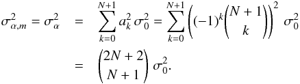10)Therefore, the quantity 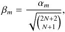${\mathit{\beta }}_{\mathit{m}}\mathrm{=}\frac{{\mathit{\alpha }}_{\mathit{m}}}{\sqrt{{{\mathrm{(}}_{\mathit{N}\mathrm{+}\mathrm{1}}^{\mathrm{2}\mathit{N}\mathrm{+}\mathrm{2}}}^{\mathrm{)}}}}\mathit{,}$(11)follows a Gaussian distribution with variance ${\mathit{\sigma }}_{\mathrm{0}}^{\mathrm{2}}$; the factor γ cancels in the calculation of β but not of α. We call a set of realizations of β a β sample. An estimate of the standard deviation of the β sample, is therefore, an estimate of the standard deviation, σ₀, of the noise term in the data.

2.3. The impact of nonequidistant sampling

In Sect. 2.2 we explicitly demanded equidistant sampling; a condition which will not always be fulfilled. We now alleviate this demand and replace it by the more lenient condition that t_{k + q}−t_k> 0 holds for any q> 0 and study whether the resulting nonequidistantly sampled measurements, y_k, can still be used in the construction of the β sample although equidistant sampling was explicitly assumed in Sect. 2.2.

As we still demand strictly and monotonically increasing t_k, there is a function E so that E(e_k) = t_k, where the e_k, again, denote equidistant points. Therefore, sampling g(t) at the points t_k is equivalent to sampling the function g_E(t) = (g°E)(t) equidistantly at the points e_k, specifically, ${\mathit{y}}_{\mathit{k}}\mathrm{=}\mathit{g}\mathrm{\left(}{\mathit{t}}_{\mathit{k}}\mathrm{\right)}\mathrm{+}{\mathit{ϵ}}_{\mathit{k}}\mathrm{=}{\mathit{g}}_{\mathit{E}}\mathrm{\left(}{\mathit{e}}_{\mathit{k}}\mathrm{\right)}\mathrm{+}{\mathit{ϵ}}_{\mathit{k}}\mathit{.}$(12)Consequently, the method remains applicable. However, the function to be locally expanded into a Taylor series would become g_E instead of g itself. Whether this proves disadvantageous for the applicability of the method depends on the specifics of the functions g and E.

In the special case that E corresponds to the inverse function of g, we obtain g_E(t) = (g°E)(t) = (g°g^-1)(t) = t, which yields a trivial Taylor expansion. Such a case appears, however, rather contrived in view of realistic data sets.

In the more general case that g corresponds to a polynomial G of degree n_p and E to a polynomial H of degree m_p, the composition g_E(t) = (G°H)(t) becomes a polynomial G_H of degree m_p × n_p. Therefore, if G is a constant (i.e., n_p = 0) any transformation of the sampling remains irrelevant because G_H remains a constant. Similarly, any linear scaling of the sampling axis (i.e., m_p = 1) leads to identical degrees for G and G_H, which remains without effect on the derivation of the noise according to Sect. 2.2. However, a more complex transformation of the sampling axis leads to an increase in the degree of the polynomial G_H. Therefore, a higher order of approximation, N, may be required to obtain acceptable results.

Missing data points, even in a series of otherwise equidistantly sampled data, pose a particular problem because the “discontinuities” introduced by them often require high polynomial degrees for H so that the resulting function, G_H, also becomes a high order polynomial even if G itself is a low order polynomial with degree ≥ 1. If such gaps in the data are sparse, the corresponding realizations of β may simply be eliminated from the β sample, and the data set can still be treated as equidistant. If the gaps are numerous or the sampling is generally heterogeneous, the application of the procedure introduced in Sect. 2.2 becomes problematic, and a more explicit treatment of the sampling is required.

2.4. Treatment of arbitrary sampling

In the general case of nonequidistant sampling, the derivation of the coefficients a_k has to be adapted. Again, we assume that t_{k + q}−t_k> 0 holds for any q> 0. In this case, Eq. (6) will assume the more general form 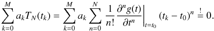$\sum _{\mathit{k}\mathrm{=}\mathrm{0}}^{\mathit{M}}{\mathit{a}}_{\mathit{k}}{\mathit{T}}_{\mathit{N}}\mathrm{\left(}{\mathit{t}}_{\mathit{k}}\mathrm{\right)}\mathrm{=}\sum _{\mathit{k}\mathrm{=}\mathrm{0}}^{\mathit{M}}{\mathit{a}}_{\mathit{k}}\sum _{\mathit{n}\mathrm{=}\mathrm{0}}^{\mathit{N}}{\frac{\mathrm{1}}{\mathit{n}\mathrm{!}}\frac{{\mathit{\partial }}^{\mathit{n}}\mathit{g}\mathrm{\left(}\mathit{t}\mathrm{\right)}}{\mathit{\partial }{\mathit{t}}^{\mathit{n}}}|}_{\mathit{t}\mathrm{=}{\mathit{t}}_{\mathrm{0}}}\mathrm{(}{\mathit{t}}_{\mathit{k}}\mathrm{-}{\mathit{t}}_{\mathrm{0}}{\mathrm{)}}^{\mathit{n}}\stackrel{\mathrm{!}}{\mathrm{=}}\mathrm{0.}$(13)In Sect. 2, we found that in the case of equidistant sampling, sets of coefficients a_k, solving the equation, can be determined for M = N + 1. As equidistant sampling is a special case of the more general situation considered here and, again, realizing that the equation must hold for any power of t_k−t₀ = t_k,0 separately, we arrive at the following linear, homogeneous system of equations for the coefficients a_k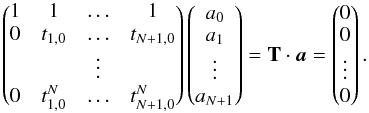$\left(\begin{array}{c}\\ \mathrm{1}& \mathrm{1}& \mathit{...}& \mathrm{1}\\ \mathrm{0}& {\mathit{t}}_{\mathrm{1}\mathit{,}\mathrm{0}}& \mathit{...}& {\mathit{t}}_{\mathit{N}\mathrm{+}\mathrm{1}\mathit{,}\mathrm{0}}\\ & & \begin{array}{c}\mathit{.}\\ \mathit{.}\\ \mathit{.}\end{array}& \\ \mathrm{0}& {\mathit{t}}_{\mathrm{1}\mathit{,}\mathrm{0}}^{\mathit{N}}& \mathit{...}& {\mathit{t}}_{\mathit{N}\mathrm{+}\mathrm{1}\mathit{,}\mathrm{0}}^{\mathit{N}}\end{array}\right)\left(\begin{array}{c}\\ {\mathit{a}}_{\mathrm{0}}\\ {\mathit{a}}_{\mathrm{1}}\\ \begin{array}{c}\mathit{.}\\ \mathit{.}\\ \mathit{.}\end{array}\\ {\mathit{a}}_{\mathit{N}\mathrm{+}\mathrm{1}}\end{array}\right)\mathrm{=}{T}\mathrm{·}{a}\mathrm{=}\left(\begin{array}{c}\\ \mathrm{0}\\ \mathrm{0}\\ \begin{array}{c}\mathit{.}\\ \mathit{.}\\ \mathit{.}\end{array}\\ \mathrm{0}\end{array}\right)\mathit{.}$(14)The solution of this system of N + 1 equations for N + 2 coefficients is a vector subspace whose dimension is given by N + 2−rank(T). Because T is a so-called Vandermonde matrix and the t_k are pairwise distinct, rank(T) is N + 1, and the dimension of the solution space is one.

By making the (arbitrary) choice a₀ = 1, we can rewrite Eq. (14) into the system 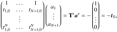$\left(\begin{array}{c}\\ \mathrm{1}& \mathit{...}& \mathrm{1}\\ {\mathit{t}}_{\mathrm{1}\mathit{,}\mathrm{0}}& \mathit{...}& {\mathit{t}}_{\mathit{N}\mathrm{+}\mathrm{1}\mathit{,}\mathrm{0}}\\ & \begin{array}{c}\mathit{.}\\ \mathit{.}\\ \mathit{.}\end{array}& \\ {\mathit{t}}_{\mathrm{1}\mathit{,}\mathrm{0}}^{\mathit{N}}& \mathit{...}& {\mathit{t}}_{\mathit{N}\mathrm{+}\mathrm{1}\mathit{,}\mathrm{0}}^{\mathit{N}}\end{array}\right)\left(\begin{array}{c}\\ {\mathit{a}}_{\mathrm{1}}\\ \begin{array}{c}\mathit{.}\\ \mathit{.}\\ \mathit{.}\end{array}\\ {\mathit{a}}_{\mathit{N}\mathrm{+}\mathrm{1}}\end{array}\right)\mathrm{=}{{T}}^{\mathrm{\prime }}{{a}}^{{\prime }}\mathrm{=}\mathrm{-}\left(\begin{array}{c}\\ \mathrm{1}\\ \mathrm{0}\\ \begin{array}{c}\mathit{.}\\ \mathit{.}\\ \mathit{.}\end{array}\\ \mathrm{0}\end{array}\right)\mathrm{=}\mathrm{-}{{t}}_{\mathrm{0}}\mathit{,}$(15)where T′ is a quadratic matrix. The solution of this system of equations can be obtained by inverting the matrix T′ so that 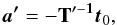${{a}}^{{\prime }}\mathrm{=}\mathrm{-}{{T}}^{\mathrm{\prime }\mathrm{-}{1}}{{t}}_{\mathrm{0}}\mathit{,}$(16)where only one column of T^′−1 is actually required. A solution to Eq. (14) reads 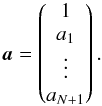${a}\mathrm{=}\left(\begin{array}{c}\\ \mathrm{1}\\ {\mathit{a}}_{\mathrm{1}}\\ \begin{array}{c}\mathit{.}\\ \mathit{.}\\ \mathit{.}\end{array}\\ {\mathit{a}}_{\mathit{N}\mathrm{+}\mathrm{1}}\end{array}\right)\mathit{.}$(17)As in the case of equidistant sampling, any multiple, γa, solves the equation, reflecting our freedom in the choice of a₀ and the dimensionality of the solution vector subspace. Using the coefficients a_k, realizations of β can be obtained analogous to Eq. (11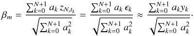${\mathit{\beta }}_{\mathit{m}}\mathrm{=}\frac{{\sum }_{\mathit{k}\mathrm{=}\mathrm{0}}^{\mathit{N}\mathrm{+}\mathrm{1}}{\mathit{a}}_{\mathit{k}}\hspace{0.17em}{\mathit{z}}_{\mathit{N,}{\mathit{t}}_{\mathit{k}}}}{\sqrt{{\sum }_{\mathit{k}\mathrm{=}\mathrm{0}}^{\mathit{N}\mathrm{+}\mathrm{1}}{\mathit{a}}_{\mathit{k}}^{\mathrm{2}}}}\mathrm{=}\frac{{\sum }_{\mathit{k}\mathrm{=}\mathrm{0}}^{\mathit{N}\mathrm{+}\mathrm{1}}{\mathit{a}}_{\mathit{k}}\hspace{0.17em}{\mathit{ϵ}}_{\mathit{k}}}{\sqrt{{\sum }_{\mathit{k}\mathrm{=}\mathrm{0}}^{\mathit{N}\mathrm{+}\mathrm{1}}{\mathit{a}}_{\mathit{k}}^{\mathrm{2}}}}\mathrm{\approx }\frac{{\sum }_{\mathit{k}\mathrm{=}\mathrm{0}}^{\mathit{N}\mathrm{+}\mathrm{1}}{\mathit{a}}_{\mathit{k}}{\mathit{y}}_{\mathit{k}}}{\sqrt{{\sum }_{\mathit{k}\mathrm{=}\mathrm{0}}^{\mathit{N}\mathrm{+}\mathrm{1}}{\mathit{a}}_{\mathit{k}}^{\mathrm{2}}}}\mathrm{·}$(18)Again, these will adhere to a Gaussian distribution with standard deviation σ₀ if the polynomial approximation is valid. Clearly, the equidistant case presented in Sect. 2.2 is a special case of this more general approach. The obvious, yet only technical, advantage of equidistant sampling is that the coefficients, a_k, need to be obtained only once, while they could be different for all subsamples in the case of arbitrary sampling.

2.5. Construction of the β sample

To estimate the standard deviation of the error term, σ₀, from data, we need to choose an order of approximation, N, and obtain realizations of β by calculating weighted sums of subsets of N + 2 data points. The question to be addressed here is how these subsets are selected.

As the order of data points is essential in the polynomial approximation, we focus on subsets of consecutive data points in the construction of the β sample. For instance, { y₁,y₂,y₃ } is a conceivable subset. To account for possible correlation between consecutive data points, we allow larger spacing between the data points by introducing a jump parameter, j, which can take any positive integer. Any subset contains the data points y_{im + kj} with 0 ≤ k<N + 2 and i_m denoting the starting index of the m^th subset. Thus, for instance { y₁,y₃,y₅ } is an admissible subset for a jump parameter of two. Depending on how the subsets are distributed (i.e., the values of the i_m are chosen) and whether they overlap, β samples with different statistical properties can be constructed.

2.5.1. Correlation in the β sample

Let K and J be two sets of N + 2 indices, each defining a subset used in the construction of the β sample. While any index must occur only once in each set, K and J may contain common indices; take as an example K₁ = { 5,6,7 } and J₁ = { 7,8,9 }. Based on K and J, realizations of β can be obtained ${\mathit{\beta }}_{\mathit{K}}\mathrm{=}\sqrt{{\mathit{f}}^{-1}}\hspace{0.17em}\sum _{\mathit{k}\mathrm{=}\mathrm{0}}^{\mathit{N}\mathrm{+}\mathrm{1}}{\mathit{a}}_{\mathit{k}}{\mathit{ϵ}}_{{\mathit{K}}_{\mathit{k}}}\mathrm{and}{\mathit{\beta }}_{\mathit{J}}\mathrm{=}\sqrt{{\mathit{f}}^{-1}}\hspace{0.17em}\sum _{\mathit{j}\mathrm{=}\mathrm{0}}^{\mathit{N}\mathrm{+}\mathrm{1}}{\mathit{a}}_{\mathit{j}}{\mathit{ϵ}}_{{\mathit{J}}_{\mathit{j}}}\mathit{,}$(19)where K_k denotes the kth element in K and $\mathit{f}\mathrm{=}\sum {\mathit{a}}_{\mathit{k}}^{\mathrm{2}}$. We also assume that the same coefficients a_k apply and the polynomial approximation holds.

The covariance, Cov, between β_K and β_J is given by $\mathrm{Cov}\left({\mathit{\beta }}_{\mathit{K}}\mathit{,}{\mathit{\beta }}_{\mathit{J}}\right)\mathrm{=}\mathit{E}\left[{\mathit{\beta }}_{\mathit{K}}\mathrm{\times }{\mathit{\beta }}_{\mathit{J}}\right]\mathrm{=}\mathit{E}\left[\frac{\mathrm{1}}{\mathit{f}}\sum _{\mathit{k}\mathrm{=}\mathrm{0}}^{\mathit{N}\mathrm{+}\mathrm{1}}\sum _{\mathit{j}\mathrm{=}\mathrm{0}}^{\mathit{N}\mathrm{+}\mathrm{1}}{\mathit{a}}_{\mathit{k}}{\mathit{a}}_{\mathit{j}}{\mathit{ϵ}}_{{\mathit{J}}_{\mathit{j}}}{\mathit{ϵ}}_{{\mathit{K}}_{\mathit{k}}}\right]\mathit{,}$(20)where E denotes the expected value. If K and J have no elements in common, the covariance is zero. If, however, K and J have a total of q elements in common and q_K,i and q_J,i denote the positions of the ith such common index in K and J, the covariance becomes $\mathrm{Cov}\mathrm{\left(}{\mathit{\beta }}_{\mathit{K}}\mathit{,}{\mathit{\beta }}_{\mathit{J}}\mathrm{\right)}\mathrm{=}\mathit{E}\left[\frac{\mathrm{1}}{\mathit{f}}\sum _{\mathit{k}\mathrm{=}\mathrm{0}}^{\mathit{N}\mathrm{+}\mathrm{1}}\sum _{\mathit{j}\mathrm{=}\mathrm{0}}^{\mathit{N}\mathrm{+}\mathrm{1}}{\mathit{a}}_{\mathit{k}}{\mathit{a}}_{\mathit{j}}{\mathit{ϵ}}_{{\mathit{J}}_{\mathit{j}}}{\mathit{ϵ}}_{{\mathit{K}}_{\mathit{k}}}\right]\mathrm{=}\frac{{\mathit{\sigma }}_{\mathrm{0}}^{\mathrm{2}}}{\mathit{f}}\sum _{\mathit{i}\mathrm{=}\mathrm{1}}^{\mathit{q}}{\mathit{a}}_{{\mathit{q}}_{\mathit{K,i}}}{\mathit{a}}_{{\mathit{q}}_{\mathit{J,i}}}\mathit{.}$(21)The previously defined sets K₁ and J₁ have the index seven in common with q_K,1 = 2 and q_J,1 = 0, which yields a covariance of $\mathrm{Cov}\left({\mathit{\beta }}_{{\mathit{J}}_{\mathrm{1}}}\mathit{,}{\mathit{\beta }}_{{\mathit{J}}_{\mathrm{1}}}\right)\mathrm{=}{\mathit{a}}_{\mathrm{2}}{\mathit{a}}_{\mathrm{0}}{\mathit{\sigma }}_{\mathrm{0}}^{\mathrm{2}}{\mathit{f}}^{-1}$.

While completely distinct index sets K and J guarantee independent realizations of β, we note that independent realizations of β can also be constructed with different index sets. For example, the sets K = { 1,2,3,4 } and J = { 3,1,4,2 }, that is, a reordering of data points, yield independent realizations of β for equidistant sampling. However, as the actual realizations of β are constructed from the data, only possibilities, which maintain the order of indices are of interest in this context.

A case of high practical importance is that of “shifted sets” by which we mean that the indices in J are computed from those in K by adding an integer s (e.g., K = { 5,6,7 } and J = { 6,7,8 } with s = 1); this is equivalent to shifting the starting point, i_m, by s data points. For 0 <s<N + 2, the resulting covariance and correlation, ρ, read $\mathrm{Cov}\mathrm{\left(}{\mathit{\beta }}_{\mathit{K}}\mathit{,}{\mathit{\beta }}_{\mathit{J}}\mathrm{\right)}\mathrm{=}\frac{{\mathit{\sigma }}_{\mathrm{0}}^{\mathrm{2}}}{\mathit{f}}\sum _{\mathit{k}\mathrm{=}\mathit{s}}^{\mathit{N}\mathrm{+}\mathrm{1}}{\mathit{a}}_{\mathit{k}}{\mathit{a}}_{\mathit{k}\mathrm{-}\mathit{s}}\mathrm{=}{\mathit{\sigma }}_{\mathrm{0}}^{\mathrm{2}}\hspace{0.17em}\mathit{\rho }\mathrm{\left(}{\mathit{\beta }}_{\mathit{K}}\mathit{,}{\mathit{\beta }}_{\mathit{J}}\mathrm{\right)}\mathit{.}$(22)In the case of evenly sampled data, the a_k have alternating sign, so that also all products a_ka_k−s have the same sign. Therefore, the covariance cannot be zero for any s<N + 2. The sign of the covariance is positive for even s and negative for odd s. Consequently, uncorrelated realizations of β cannot be obtained from overlapping shifted subsets of data points.

2.5.2. Obtaining independent realizations of β

Realizations of β are independent if any data point is used only in one realization (Sect. 2.5.1). For a jump parameter of one (i.e., consecutive data points), the most straight-forward approach to construct such a β sample is to divide the data set into subsets of N + 2 consecutive data points so that the first subset comprises the points y₀...y_{N + 1}, the second one the points y_{N + 2}...y_{2 × (N + 2)−1}, and so on. Incomplete sets with less than N + 2 points are disregarded.

If a larger jump parameter is specified, we define consecutive chunks of (N + 2) × j points and subdivide them into j subsets by collecting all points for which i mod j = l, where i is the index of the point and 0 ≤ l<j. Table 1 demonstrates a number of subdivisions following this procedure. The size of the resulting β sample will approximately be given by n_d (N + 2)^-1 not accounting for potentially neglected points in incomplete subsets.

2.5.3. Obtaining correlated realizations of β by shifting

A β sample can be constructed by assigning the data points y_{i0 + kj} (0 ≤ k<N + 2) to the first subset and then increase i₀ from zero to n_d−j × (N + 1)−1 in steps of one. The effect is that of shifting the subsets across the data. In this way, all data points will occur in the β sample at least once.

The size of the β sample obtainable in this fashion is n_d−j × (N + 1), which hardly depends on the order of approximation and can be substantially larger than the sample of independent realizations of β. However, these realization are correlated (Sect. 2.5.1).

2.6. Estimating the variance and standard deviation

The procedure used to estimate the standard deviation of the β sample remains immaterial for the concept of the method and can be chosen to fit the purpose best. The usual variance estimators² are $\begin{array}{ccc}\mathit{ŝ}\mathrm{2}\mathrm{\left(}\mathit{B}\mathrm{\right)}& \mathrm{=}& \frac{\mathrm{1}}{\mathit{n}\mathrm{-}\mathrm{1}}\sum _{\mathit{i}\mathrm{=}\mathrm{1}}^{\mathit{n}}\mathrm{(}{\mathit{\beta }}_{\mathit{i}}\mathrm{-}\overline{\mathit{\beta }}{\mathrm{)}}^{\mathrm{2}}\mathrm{and}\\ \mathit{ŝ}\begin{array}{c}\mathrm{2}\\ \mathit{E}\end{array}\mathrm{\left(}\mathit{B}\mathrm{\right)}& \mathrm{=}& \frac{\mathrm{1}}{\mathit{n}}\sum _{\mathit{i}\mathrm{=}\mathrm{1}}^{\mathit{n}}\mathrm{(}{\mathit{\beta }}_{\mathit{i}}\mathrm{-}\mathit{E}\mathrm{[}\mathit{\beta }\mathrm{]}{\mathrm{)}}^{\mathrm{2}}\mathit{,}\end{array}$where E [β] denotes the expectation value of β and n is the sample size. Using ŝ², the expectation value is estimated from the sample by the mean, $\overline{\mathit{\beta }}$. While E [β] is zero by construction, in working with real data, the assumptions leading to this result may not be completely fulfilled, so that both can be useful in the analysis. For independent, Gaussian β samples, both ŝ² and $\mathit{ŝ}\begin{array}{c}\mathrm{2}\\ \mathit{E}\end{array}$ are unbiased. In the case of correlated samples however, only $\mathit{ŝ}\begin{array}{c}\mathrm{2}\\ \mathit{E}\end{array}$ remains so, while ŝ² generally becomes biased (Bayley & Hammersley 1946).

The variance, V, of the estimator $\mathit{ŝ}\begin{array}{c}\mathrm{2}\\ \mathit{E}\end{array}$ reads (Bayley & Hammersley 1946) $\mathit{V}\mathrm{(}\mathit{ŝ}{\begin{array}{c}\mathrm{2}\\ \mathit{E}\end{array}}^{\mathrm{)}}\mathrm{=}\frac{\mathrm{2}{\mathit{\sigma }}^{\mathrm{4}}}{\mathit{n}}\mathrm{+}\frac{\mathrm{4}{\mathit{\sigma }}^{\mathrm{4}}}{{\mathit{n}}^{\mathrm{2}}}\sum _{\mathit{j}\mathrm{=}\mathrm{1}}^{\mathit{N}\mathrm{+}\mathrm{2}}\mathrm{(}\mathit{n}\mathrm{-}\mathit{j}\mathrm{)}{\mathit{\rho }}_{\mathit{j}}^{\mathrm{2}}\mathrm{\approx }\frac{\mathrm{2}{\mathit{\sigma }}^{\mathrm{4}}}{\mathit{n}}\left(\mathrm{1}\mathrm{+}\mathrm{2}\sum _{\mathit{j}\mathrm{=}\mathrm{1}}^{\mathit{N}\mathrm{+}\mathrm{2}}{\mathit{\rho }}_{\mathit{j}}^{\mathrm{2}}\right)\mathit{,}$(25)where ρ_j is the correlation at an offset of j in the β sample, and the approximation holds for N + 2 ≪ n.

The square root of the variance estimator, ŝ_E(B), is an estimator of the standard deviation. We note however, that it is not unbiased. For independent Gaussian samples the expectation value of ŝ_E becomes $\mathit{E}\left[\mathit{ŝ}\mathit{E}\mathrm{\left(}\mathit{B}\mathrm{\right)}\right]\mathrm{=}{\mathit{\sigma }}_{\mathrm{0}}\sqrt{\frac{\mathrm{2}}{\mathit{n}}}\hspace{0.17em}\frac{\mathrm{\Gamma }\mathrm{(}{\frac{\mathit{n}}{\mathrm{2}}}^{\mathrm{)}}}{\mathrm{\Gamma }\mathrm{(}{\frac{\mathit{n}\mathrm{-}\mathrm{1}}{\mathrm{2}}}^{\mathrm{)}}}\mathrm{\approx }{\mathit{\sigma }}_{\mathrm{0}}\left(\mathrm{1}\mathrm{-}\frac{\mathrm{3}}{\mathrm{4}\mathit{n}}\right)\mathit{,}$(26)where Γ denotes the gamma function (see Forbes et al. 2011; Kenney 1940, Chap. VII). The bias decreases as the inverse of the number of independent samples, which is, however, not trivially obtained in the case of correlated samples (Bayley & Hammersley 1946).

In many practical cases, expectation biases are a minor issue because, first, they tend to decrease with sample size for Gaussian samples, and second, the assumption of independent Gaussian errors will generally only hold approximately. We will use s_E as an estimate of the standard deviation of the error term and approximate the standard deviation, σ_sE, of the estimate by error propagation based on the variance of ${\mathit{s}}_{\mathit{E}}^{\mathrm{2}}$, that is, ${\mathit{\sigma }}_{{\mathit{s}}_{\mathit{E}}}\mathrm{=}\sqrt{\frac{\mathit{V}\mathrm{(}{{\mathit{s}}_{\mathit{E}}^{\mathrm{2}}}^{\mathrm{)}}}{\mathrm{4}{\mathit{s}}_{\mathit{E}}^{\mathrm{2}}}}\mathrm{·}$(27)Frequently, the data contain grossly misplaced data points in stark contrast with the distribution of the remaining ensemble of points, which have to be dealt with. Such points are usually referred to as outliers. Because the breakdown point of the estimator $\mathit{ŝ}\begin{array}{c}\mathrm{2}\\ \mathit{E}\end{array}$ is zero (Hampel 1974), a single such outlier can be sufficient to spoil the estimate obtained from it and, thus, render the result useless. In such cases, a more robust estimator is desirable.

Among the most robust estimators of the standard deviation is the “median absolute deviation about the median” (MAD). The estimator is given by $\begin{array}{ccc}\mathit{ŝ}\mathrm{M}\mathrm{\left(}\mathit{B}\mathrm{\right)}& \mathrm{=}& \mathit{k}\mathrm{\times }\mathrm{med}\mathit{i}\mathrm{(}{\left|\hspace{0.17em}{\mathit{\beta }}_{\mathit{i}}\mathrm{-}\mathrm{med}\mathit{j}\mathrm{\left(}{\mathit{\beta }}_{\mathit{j}}\mathrm{\right)}\hspace{0.17em}\right|}^{\mathrm{)}}\mathrm{and}\\ \mathit{ŝ}\mathrm{ME}\mathrm{\left(}\mathit{B}\mathrm{\right)}& \mathrm{=}& \mathit{k}\mathrm{\times }\mathrm{med}\mathit{i}\left(\left|\hspace{0.17em}{\mathit{\beta }}_{\mathit{i}}\hspace{0.17em}\right|\right)\mathit{,}\end{array}$where the constant k is about 1.4826 (Hampel 1974; Rousseeuw & Croux 1993). Again, we can take advantage of the known median of the β sample. While ŝ_M(B) is a robust estimator for the standard deviation with the maximal breakdown point of 0.5, its asymptotic efficiency in the case of normally distributed samples is only 37% (Hampel 1974; Rousseeuw & Croux 1993). The price for a more robust estimate is therefore efficiency. The estimator ŝ_M(B) is consistent (Rousseeuw & Croux 1993) and thus, asymptotically unbiased. Besides ŝ_M(B), a number of alternative, robust estimators with partly higher efficiency have been given in the literature (Rousseeuw & Croux 1993), either of which could be used to estimate the standard deviation of the β sample. In the following, we will concentrate on ŝ_E(B) and ŝ_ME(B) and refer to these estimators as the minimum variance (MV) and the robust estimator.

2.7. Relation to the DER_SNR algorithm

At this point, we have assembled all pieces to see the relation to the DER_SNR algorithm presented by Stoehr et al. (2008). If the order of approximation is one, the jump parameter is two, a correlated β sample is constructed by the shifting technique, and ŝ_ME is used to estimate the standard deviation from it, the βσ procedure becomes identical to the DER_SNR algorithm presented by Stoehr et al. (2008), given that the data are equidistantly sampled (see Sect. 1).

2.8. An upper limit on the amplitude of noise

Even if the noise distribution is normal and an unbiased estimator for the standard deviation is used, the expectation value of the noise estimate is only identical to σ₀ as long as y_i = z_N,i or, equivalently, the polynomial approximation is exact T_N(t_i) = g(t_i). If this is not the case, so that y_i−T_N(t_i) = ϵ_i + r_N,i with some non-negligible remainder r_N,i, the noise estimate may no longer remain unbiased. Even in the case of ϵ_i = 0, the expectation value will then generally be larger than zero because the ϵ_i are independent of the r_N,i and their variances will add. While the expectation value of the estimator therefore, cannot be smaller than σ₀, we note that this may still be the case for individual estimates.

2.9. Relative efficiency of the estimator

The variance of the estimator $\mathit{ŝ}\begin{array}{c}\mathrm{2}\\ \mathit{E}\end{array}$ and thus, its efficiency depend on the size of the β sample and the correlation between its elements. If an independent β sample is constructed, its sample size is approximately given by n_d × (N + 2)^-1. For the lowest order of approximation (i.e., zero), the variance of ${\mathit{s}}_{\mathit{E}}^{\mathrm{2}}$ obtained from this sample reads $\mathrm{4}{\mathit{\sigma }}_{\mathrm{0}}^{\mathrm{4}}{\mathit{n}}_{\mathrm{d}}^{-1}$. If ${\mathit{s}}_{\mathit{E}}^{\mathrm{2}}$ is calculated from the β sample obtained by the shifting procedure, the sample size is approximately n_d, and the variance reads $\mathrm{2}{\mathit{\sigma }}_{\mathrm{0}}^{\mathrm{4}}{\mathit{n}}_{\mathrm{d}}^{-1}\mathrm{(}\mathrm{1}\mathrm{+}\mathrm{0.5}\mathrm{)}\mathrm{=}\mathrm{3}{\mathit{\sigma }}_{\mathrm{0}}^{\mathrm{4}}{\mathit{n}}_{\mathrm{d}}^{-1}$. We note, however, that this result only applies for equidistant sampling.

When orders of approximation N₁ and N₂ are used with an independent β sample, the ratio of the variances, V, of the estimators $\mathit{ŝ}\begin{array}{c}\mathrm{2}\\ \mathit{E}\end{array}\mathrm{\left(}{\mathit{N}}_{\mathrm{1}\mathit{,}\mathrm{2}}\mathrm{\right)}$ reads $\frac{\mathit{V}\mathrm{\left(}\mathit{ŝ}\begin{array}{c}\mathrm{2}\\ \mathit{E}\end{array}\mathrm{\right(}{\mathit{N}}_{\mathrm{1}}{\mathrm{\left)}}^{\mathrm{\right)}}}{\mathit{V}\mathrm{\left(}\mathit{ŝ}\begin{array}{c}\mathrm{2}\\ \mathit{E}\end{array}\mathrm{\right(}{\mathit{N}}_{\mathrm{2}}{\mathrm{\left)}}^{\mathrm{\right)}}}\mathrm{=}\frac{{\mathit{N}}_{\mathrm{1}}\mathrm{+}\mathrm{2}}{{\mathit{N}}_{\mathrm{2}}\mathrm{+}\mathrm{2}}\mathrm{·}$(30)If a correlated β sample is constructed using the shifting algorithm, its size hardly depends on the order of approximation given that n_d ≫ N + 2. Due to the correlation, this does not translate into identical efficiency, however. In Fig. 1, we show the variance of $\mathit{ŝ}\begin{array}{c}\mathrm{2}\\ \mathit{E}\end{array}$ for various orders of approximation, relative to $\mathrm{3}{\mathit{\sigma }}_{\mathrm{0}}^{\mathrm{4}}{\mathit{n}}_{\mathrm{d}}^{-1}$.

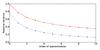Fig. 1 Minimum variance of $\mathrm{3}{\mathit{\sigma }}_{\mathrm{0}}^{\mathrm{4}}{\mathit{n}}_{\mathrm{d}}^{-1}$ for $\mathit{ŝ}\begin{array}{c}\mathrm{2}\\ \mathit{E}\end{array}$ divided by variance obtained for various orders of approximation for independent (dashed blue) and correlated β samples (solid red).

Higher orders of approximation always worsen the relative asymptotic efficiency of the estimator due to the decrease in sample size and the impact of correlation. The results obtained from the correlated β sample are always superior in terms of efficiency for the same order of approximation. The correlation structure considered here, however, only applies for equidistant sampling of the data.

2.10. Correlation between estimates of different order

Given a sample of independent realizations of a Gaussian random variable, the conditions for the βσ procedure to yield reliable estimates are fulfilled for all orders of approximation. Here, we demonstrate that estimates obtained with different orders of approximation are highly correlated.

To this end, we obtain a sample of 1000 independently sampled Gaussian random numbers and estimate their variance by using β samples constructed using the shifting technique and orders of approximation between zero and four. Repeating this experiment 5000 times, we estimate the correlation of the thus derived noise variance estimates and summarize the results in Table 2; for clarity we omit the symmetric part of the table. Clearly, high degrees of correlation are ubiquitous.

Practically, this implies that estimates based on different (and especially subsequent) orders of approximation differ less than suggested by their nominal variance, if the order of approximation is sufficient to account for the systematic variation in the data. As the estimates are based on the same input data, this behavior may of course be expected. Naturally, the correlation depends on the construction of the β sample. For example, if an independent β sample is constructed, the correlation is still significant but lower with correlation coefficients around 0.5.

3. Python implementation of βσ procedure

Along with this presentation, we provide a set of Python routines implementing the βσ procedure as outlined here. The code is available both as a stand-alone module and as part of our PyAstronomy package available via the github platform³.

The code runs under both Python 2.7 and the 3.x series and comes with documentation and examples of application. It provides algorithms to derive independent and correlated β samples based on both equidistantly sampled and arbitrarily sampled data sets. Our implementation is distributed under the MIT license⁴ inviting use and modification by all interested parties. The routines are also used in the applications presented in the following Sect. 4.

4. Application to real and synthetic data

In the following we apply the βσ procedure to estimate the amplitude of noise in synthetic data, high-resolution echelle spectra, and a sample of space-based CoRoT light curves to demonstrate its applicability in real-world scenarios.

4.1. Application to synthetic data

We start by determining the noise in a series of synthetic data sets generated from the function 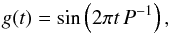$\mathit{g}\mathrm{\left(}\mathit{t}\mathrm{\right)}\mathrm{=}\sin \mathrm{(}\mathrm{2}\mathit{\pi t}\hspace{0.17em}{\mathit{P}}^{-1}\mathrm{)}\mathit{,}$(31)sampled at a total of 1000 equidistant points given by t_i = 0.1 × i (0 ≤ i< 1000) so that Δt = 0.1. In our calculations, we use a number of different periods, P, to demonstrate the effect of different sampling rates. Specifically, a single oscillation is sampled by PΔt^-1 data points. To each data set, we add a Gaussian noise term with a standard deviation of σ₀ = 0.1.

From the synthetic data sets we derive estimates of the known input standard deviation, σ₀, constructing correlated β samples using various orders of approximation and the shifting procedure. For each combination of period and order of approximation, we repeat the experiment 200 times and record the resulting estimates of the standard deviation, s_E, its estimated standard error, σ_sE, and the relative deviation from the known value $\mathit{d}\mathrm{=}\mathrm{(}{\mathit{s}}_{\mathit{E}}\mathrm{-}{\mathit{\sigma }}_{\mathrm{0}}\mathrm{)}\hspace{0.17em}{\mathit{\sigma }}_{{\mathit{s}}_{\mathit{E}}}^{-1}$. In Table 3 we show the thus derived expected relative deviation of the estimate from the true value for orders of approximation 0 ≤ N ≤ 5. Lower orders of approximation suffice in the case of well sampled curves for which PΔt^-1 is large. As the sampling of the oscillation becomes more sparse, the required order of approximation rises. These effects are clearly seen in Table 3.

4.1.1. A pathological case

A pathological case in the sense of convergence of the βσ procedure is the data set y_i = (−1)ⁱ, which could, for example, have been obtained by sampling only the minima and maxima of an underlying oscillation. In this example, we assume a noise-free data set. For any odd jump parameter, all realizations of β will have the same value 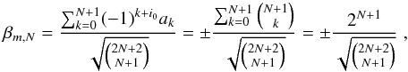${\mathit{\beta }}_{\mathit{m,N}}\mathrm{=}\frac{{\sum }_{\mathit{k}\mathrm{=}\mathrm{0}}^{\mathit{N}\mathrm{+}\mathrm{1}}\mathrm{(}\mathrm{-}\mathrm{1}{\mathrm{)}}^{\mathit{k}\mathrm{+}{\mathit{i}}_{\mathrm{0}}}{\mathit{a}}_{\mathit{k}}}{\sqrt{{{\mathrm{(}}_{\mathit{N}\mathrm{+}\mathrm{1}}^{\mathrm{2}\mathit{N}\mathrm{+}\mathrm{2}}}^{\mathrm{)}}}}\mathrm{=}\mathrm{\pm }\frac{{\sum }_{\mathit{k}\mathrm{=}\mathrm{0}}^{\mathit{N}\mathrm{+}\mathrm{1}}{{\mathrm{(}}_{\mathit{k}}^{\mathit{N}\mathrm{+}\mathrm{1}}}^{\mathrm{)}}}{\sqrt{{{\mathrm{(}}_{\mathit{N}\mathrm{+}\mathrm{1}}^{\mathrm{2}\mathit{N}\mathrm{+}\mathrm{2}}}^{\mathrm{)}}}}\mathrm{=}\mathrm{\pm }\frac{{\mathrm{2}}^{\mathit{N}\mathrm{+}\mathrm{1}}}{\sqrt{{{\mathrm{(}}_{\mathit{N}\mathrm{+}\mathrm{1}}^{\mathrm{2}\mathit{N}\mathrm{+}\mathrm{2}}}^{\mathrm{)}}}}\mathit{,}$(32)where the sign depends on whether the starting index, i₀, of the subsample is even or odd.

When the order of approximation is increased by one, the value of the corresponding realizations of β grows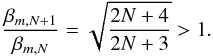$\frac{{\mathit{\beta }}_{\mathit{m,N}\mathrm{+}\mathrm{1}}}{{\mathit{\beta }}_{\mathit{m,N}}}\mathrm{=}\sqrt{\frac{\mathrm{2}\mathit{N}\mathrm{+}\mathrm{4}}{\mathrm{2}\mathit{N}\mathrm{+}\mathrm{3}}}\mathit{>}\mathrm{1.}$(33)If the number of data points is sufficiently large to apply arbitrary orders of approximation, N, it can be shown that the variance estimate, ${\mathit{s}}_{\mathit{E}}^{\mathrm{2}}$, increases without bounds. Specifically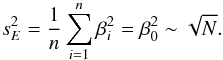, ${\mathit{s}}_{\mathit{E}}^{\mathrm{2}}$ grows as${\mathit{s}}_{\mathit{E}}^{\mathrm{2}}\mathrm{=}\frac{\mathrm{1}}{\mathit{n}}\sum _{\mathit{i}\mathrm{=}\mathrm{1}}^{\mathit{n}}{\mathit{\beta }}_{\mathit{i}}^{\mathrm{2}}\mathrm{=}{\mathit{\beta }}_{\mathrm{0}}^{\mathrm{2}}\mathrm{~}\sqrt{\mathit{N}}\mathit{.}$(34)Although the case here considered is somewhat contrived, it clearly demonstrates that, first, there may be cases when the βσ procedure does not converge to the true value of the noise for any order of approximation and, second, that estimates obtained from consecutive orders of approximation may be arbitrarily close nonetheless. However, the fact that the estimates continuously grow for increasing orders of approximation clearly indicates that no improvement is achieved and the underlying approximations may be violated. In this specific case, we note that for even jump parameter all realizations of β are zero and the correct result would be derived, which is due to the special construction of the problem considered here.

4.2. Application to high-resolution spectra

We obtain estimates of the noise in high-resolution echelle spectra of HR 7688 and HD 189733 obtained with the UVES spectrograph⁵. In our analysis, we adopted the 6070−6120 Å range. The corresponding spectra are shown in Fig. 2. The data reduction is based on the UVES pipeline and is described in Czesla et al. (2015).

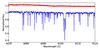Fig. 2 Normalized spectrum of HR 7688 (red, shifted by +0.2) and HD 189733 (blue).

First, we estimate the noise in the spectrum of the fast-rotating B3V star HR 7688, which shows no narrow spectral features and served as a telluric standard. In Fig. 3, we show the estimated standard deviation of the noise, obtained for different orders of approximation and jump parameters, using the MV estimator; the β sample was constructed using the shifting procedure. The estimates obtained for a jump parameter of one clearly converge to a lower value for increasing orders of approximation than those for larger jump parameters. As the data do not show strong spectral lines, we attribute this behavior to correlation in the noise of adjacent data points, so that the assumption of mutually independent realizations of noise is violated. For larger jump parameters the estimates hardly vary as a function of the order of approximation, showing the high degree of correlation demonstrated in Sect. 2.10. Valid estimates are thus only obtained for jump parameters larger than one; all such estimates for HR 7688 considered in our analysis shown in Fig. 3 are essentially consistent. The picture obtained by using the robust estimator is very similar.

Combining the estimate of (884 ± 14) × 10^-16 erg cm^-2 Å^-1 s^-1 obtained for the zeroth order of approximation and a jump parameter of three with the median flux density in the studied spectral range, we obtain an estimate of 209 ± 4 for the signal-to-noise ratio. The estimates based on the MV and robust estimators provide consistent results and, naturally, also the DER_SNR estimate is compatible with this value. While this result appears to be consistent with an estimated scatter of 993 × 10^-16 erg cm^-2 Å^-1 s^-1 in the residuals after a fourth order polynomial approximation of the entire considered range, the mean pipeline estimate of about 1500 erg cm^-2 Å^-1 s^-1 appears to be on the conservative side. As a cross-check of our estimate, we added uncorrelated noise with a standard deviation of 500 erg cm^-2 Å^-1 s^-1 to the data. This yielded a noise estimate of 1017 ± 14 erg cm^-2 Å^-1 s^-1 for the same order of approximation and jump parameter, which is consistent with the sum of variances.

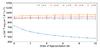Fig. 3 Noise estimate as a function of order of approximation, N, and jump parameter, j, for HR 7688.

In Fig. 4, we show the noise estimates obtained from the spectrum of the K-type star HD 189733 using the MV estimator, ŝ_E, and the robust estimator, ŝ_ME. For a jump parameter of one, the estimates again converge to a lower value than for larger jump parameters, which we attribute to correlation. The series of estimates obtained with the robust estimator show a much better convergence behavior toward higher orders of approximation. In particular, lower orders of approximation tend to yield significantly smaller robust estimates; we emphasize the difference in scale in the top and bottom panel.

While for jump parameters of two and three, both the MV and robust estimates converge toward a value of about 150 erg cm^-2 Å^-1 s^-1, larger jump parameters systematically yield larger estimates. We attribute this behavior to the structure seen in the spectrum, that is, the spectral lines. The larger the jump parameter, the longer the sections of the spectrum, which have to be approximated by a polynomial of the same degree.

To obtain reliable error estimates, a jump parameter of two or three and an order of approximation larger than about four appear necessary in this case. Adopting the robust estimate s_ME(N = 5,j = 2) of (156 ± 4) × 10^-16 erg cm^-2 Å^-1 s^-1, we obtain a signal-to-noise estimate of 205 ± 8 in the considered spectral range. We approximate the variance of the robust estimator by scaling that of the efficient estimator with a factor of 2.7, in accordance with their asymptotic efficiencies. Again, the MV and robust estimates are consistent. Using the DER_SNR in its original form (i.e., N = 1 and j = 2) yields a robust noise estimate about 20% larger than the value adopted here.

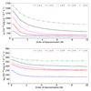Fig. 4 Noise estimates for the spectrum of HD 189733 as a function of order of approximation, N, and jump parameter, j, for efficient (top) and robust (bottom) estimator.

From the above, it is clear that reliable noise estimates need some scrutiny. In the case at hand, the availability of the spectrum of HR 7688 is of great help because it allows us to study the noise properties in a reference data set largely free of any underlying variability, which immediately reveals the peculiarity of the results for unity jump parameter. Nonetheless, also given the data of HD 189733 alone, this would have been recognized, and a reliable estimate could have been derived.

4.3. Application to CoRoT data

Next, we obtain estimates of the noise contribution in a sample of CoRoT light curves using the βσ procedure. Specifically, we analyze all 1640 short-cadence light curve from the fourth long run, targeting the galactic anticenter (LRa04, e.g., Auvergne et al. 2009). Because the number of data points per light curve is large (≈180 000), we construct independent β samples. Estimates obtained using an order of approximation, N and jump parameter, j, are denoted by ${}^{\mathit{\beta }}\mathit{\sigma }_{\mathit{N,j}}$.

To determine the required order of approximation and the jump parameter, we apply the following procedure: first, we use an order of approximation of zero and a jump parameter of one and obtain the estimates ${}^{\mathit{\beta }}\mathit{\sigma }_{\mathit{N,j}}$, ${}^{\mathit{\beta }}\mathit{\sigma }_{\mathit{N}\mathrm{+}\mathrm{1}\mathit{,j}}$, and ${}^{\mathit{\beta }}\mathit{\sigma }_{\mathit{N}\mathrm{+}\mathrm{1}\mathit{,j}\mathrm{+}\mathrm{1}}$ using the robust estimator, taking into account irregular sampling. Second, we check whether the three estimates are consistent, which we define to be the case when their three sigma confidence intervals overlap. Again, we approximate the variance of the robust estimator by scaling that of the MV estimator in accordance with their asymptotic efficiencies. If ${}^{\mathit{\beta }}\mathit{\sigma }_{\mathit{N,j}}$ and ${}^{\mathit{\beta }}\mathit{\sigma }_{\mathit{N}\mathrm{+}\mathrm{1}\mathit{,j}}$ are inconsistent, we increase the order of approximation by one and restart the procedure. If ${}^{\mathit{\beta }}\mathit{\sigma }_{\mathit{N,j}}$ and ${}^{\mathit{\beta }}\mathit{\sigma }_{\mathit{N}\mathrm{+}\mathrm{1}\mathit{,j}\mathrm{+}\mathrm{1}}$ are inconsistent, we increase both the order of approximation and the jump parameter by one and restart the procedure. If ${}^{\mathit{\beta }}\mathit{\sigma }_{\mathit{N,j}}$ is consistent with the other two estimates, we stop the iteration.

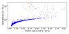Fig. 5 Estimated standard deviation of noise as a function of median signal in the LRa04 short-cadence light curves obtained by CoRoT (blue dots). Red points indicate light curves for which our iterative procedure yielded an order of approximation larger than two.

For 1499 out of 1640 light curves, the zeroth order of approximation remained sufficient according to our criterion, 33 required the first, and 88 the second order; in 20 cases a higher order was required. In Fig. 5 we show the resulting noise estimate as a function of the median flux in the light curve. The distribution shows that the noise contribution qualitatively follows a square-root relation with respect to the median flux, which is indicative of a dominant Poisson noise contribution. The results in Fig. 5 have been derived allowing for arbitrary sampling, however, the majority of robust estimates obtained assuming regular sampling are identical. If there is a difference, estimates based on equidistant sampling tend to be larger by typically less than a percent. Compared to the estimates obtained using the MV estimator, the robust estimates tend to be lower by a few percent for the order of approximation and jump parameter at which the iterative procedure halted.

A number of light curves apparently show noise levels significantly above the square-root relation outlined by the majority of noise estimates. In Fig. 5, we indicate those light curves for which our iterative procedure halted at an order of approximation larger than two. While the corresponding light curves tend to be those with higher noise levels, there is no unique mapping. We checked our result using, first, a comparison with the noise level estimated using the standard derivation of the residuals obtained from a second-order polynomial fit to the first 200 data points in each light curve. The noise estimates obtained with this method are on average 6% higher than those derived using the βσ procedure with a number of estimates off by a factor of a few. Yet, the result confirms the reality of the outliers. Second, a visual inspection confirmed a comparatively large scatter in the light curves, consistent with the obtained estimates. Light curves showing increased noise levels were also reported on by Aigrain et al. (2009), who studied the noise in CoRoT light curves on the transit timescale.

As an example, Fig. 6 shows the light curves of the stars with CoRoT IDs 605144111 and 605088599, which both show similar median flux levels of 1.06 × 10⁶ e⁻(32s)^-1. While the estimated scatter in the first is consistent with the square-root relation, the second is a factor of 6.8 larger. For this star, Fig. 6 shows both a larger level of (apparently) stochastic variability between individual data points (bottom panel) and a higher degree of overall variability in the 80 d long light curve (top panel), which remains, however, irrelevant in the noise estimation. In fact, the light curve of CoRoT 605088599 is among the few for which our procedure halted only at an order of approximation of seven with a jump parameter of six.

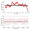Fig. 6 Light curves of the stars with CoRoT IDs 605144111 (black) and 605088599 (red). Top panel: entire available light curve with a temporal binning of 30 min. Bottom panel: excerpt of the light curves with original binning of 32 s (black dots for CoRoT IDs 605144111 and red triangles for 605088599).

The behavior of the outlier light curves may be due to an additional source of random noise or a highly variable stochastic component in the light curve both either of instrumental or physical origin. The βσ procedure provides an estimate of the standard deviation of the stochastic contribution in the data as specified in Sect. 2; it neither distinguishes between individual sources of that term nor does it tell us anything about its origin in itself. It is also conceivable that actual convergence has not been achieved in some cases (see Sect. 4.1.1). While an in-depth analysis of the peculiar light curves forming the class of outliers is beyond the scope of this discussion, the presented procedure proved highly robust in estimating the amplitude of noise in a large sample of light curves with a wide range of morphologies.

5. Setting up the βσ procedure

The βσ procedure as presented here is a concept, requiring a number of choices to be made prior to application. Specifically, the order of approximation and the jump parameter have to be selected, a strategy to construct the β sample has to be chosen, and an estimator to determine the standard deviation (or variance) of the β sample needs to be specified. A number of options, but certainly not all, have been discussed above.

Clearly, the optimal choice depends on the data set at hand, and our decision may be guided by the information we have about the data, such as a typical scale of variation compared to the sampling cadence. While it can be shown under which conditions the βσ (or DER_SNR) estimates are reliable, we do not see a possibility to prove that the method yielded the correct result based on the result itself.

In fact, any set of N + 2 measurements may also be described by a polynomial of degree N + 1 with no random noise contribution at all. If g(t) is a function showing N or more extrema in the range covered by the N + 2 data points such as a higher-order polynomial or fast oscillation, the proposed estimator will generally be biased because an Nth order polynomial approximation remains no longer appropriate. Nonetheless, useful strategies and recipes can be defined to strengthen the confidence in the outcome.

5.1. Choosing the order of approximation and the jump parameter

The required order of approximation is mainly determined by the degree of variability seen in the data with respect to the sampling rate. Slowly varying (or better sampled) data sets require lower orders of approximation. The larger the jump parameter is chosen, the longer become the sections of the data, which have to be modeled using the same order of approximation. If correlation in the noise distribution is known, it is advisable to opt for a jump parameter larger than the correlation scale.

Based on our experience, we propose to obtain at least two estimates with consecutive orders of approximation and accept the values only if both estimates are consistent. If the conditions for the method to be applicable hold, the estimates obtained using consecutive orders of estimates are expected to yield statistically indistinguishable results (Sect. 2.10). If this is not the case, a higher order of approximation may be required to account for the intrinsic variation in the data, and the order should be increased by one. Unless other prior information is available, we suggest to start with the lowest orders of approximation (zero and one). At any rate, the consistency of estimates obtained with different orders of approximation is not a sufficient condition for a valid estimate (Sect. 4.1.1).

Additionally, we suggest to carry out a cross-check of the result using a a larger jump parameter to exclude effects, for example, attributable to correlation between the noise in adjacent data points. Such an effect was observed in our study of the high-resolution spectra (Sect. 4.2) and was also discussed by Stoehr et al. (2008). No such effect appears to be present in the CoRoT data (Sect. 4.3).

5.2. Selecting an estimator

For well-behaved, Gaussian β samples, the estimator used to obtain the standard deviation remains of little practical significance. In working with real data, it appears that the main choice is between robust and non-robust techniques. While the robust estimators are typically of smaller efficiency (for Gaussian samples), we attribute the main problems in our applications to outliers and non-Gaussian samples. Our results suggest that robust estimates are more reliable. We caution that in the case of small β samples, estimation biases may become an issue to be kept in mind.

5.3. Construction of the β sample

We discussed procedures to construct both β samples with independent and correlated elements. We found the estimates derived from the correlated β samples, constructed using the shifting technique, superior in many applications because they preserve a larger fraction of the information contained in the data. The uncorrelated β samples are smaller in size and give rise to less precise noise estimates. Nonetheless, independent samples may still be useful, for example, if estimation biases due to correlation shall be excluded or the number of data points is large (Sect. 4.3).

6. Conclusion

The βσ procedure presented here is a versatile technique to estimate the amplitude of noise in discrete data sets, which can be proved to work for sufficiently well-sampled data sets. It is related to numerical differentiation and differencing as regularly applied in time series analyses (Shumway & Stoffer 2006). Also polynomial approximations have been used for a long time, for example, in the context of the Savitzky-Golay filter (Savitzky & Golay 1964). However, we are not aware of an application of the presented procedure in astronomy other than in the form of the DER_SNR algorithm by Stoehr et al. (2008); in fact, the βσ procedure is the DER_SNR algorithm for a specific choice of parameters.

We provide an analysis of the statistical properties of the resulting noise estimates, depending on the chosen parameters for the βσ procedure and applied it to synthetic data, high-resolution spectra, and a large sample of CoRoT light curves. While the conditions for the procedure to work can clearly be spelled out, a difficulty in the application arises from the fact that we cannot show the validity of the noise estimate by application of the procedure itself.

In our test applications, we address this problem by comparison of estimates obtained from a number of β samples, constructed using different orders of approximation and jump parameters. Noise estimates are only accepted if they are consistent. Unless other external information is available about the data, this is also the recipe we suggest to be used in the general case of application. In our test cases, robust estimation proved to be advantageous in determining the amplitude of noise. While we agree with Stoehr et al. (2008) that the settings of the DER_SNR algorithm (i.e., N = 1 and j = 2) are reliable in many cases, we cannot generally conclude that this will be the case for any data set. Therefore, we suggest to verify the result by comparing it with that obtained using the next higher order of approximation and eventually, also a larger (or smaller) jump parameter.

Along with this paper, we provide a Python implementation of the βσ procedure, open for use and modification by all interested parties. The βσ procedure is highly versatile and once the properties of the data are approximately known, it can be applied to derive the amplitude of noise in large samples without further interference.

Acknowledgments

We thank the anonymous referee for knowledgeable comments, which helped to improve our paper.

References

All Tables

All Figures

	Fig. 1 Minimum variance of $\mathrm{3}{\mathit{\sigma }}_{\mathrm{0}}^{\mathrm{4}}{\mathit{n}}_{\mathrm{d}}^{-1}$ for $\mathit{ŝ}\begin{array}{c}\mathrm{2}\\ \mathit{E}\end{array}$ divided by variance obtained for various orders of approximation for independent (dashed blue) and correlated β samples (solid red).
In the text

	Fig. 2 Normalized spectrum of HR 7688 (red, shifted by +0.2) and HD 189733 (blue).
In the text

	Fig. 3 Noise estimate as a function of order of approximation, N, and jump parameter, j, for HR 7688.
In the text

	Fig. 4 Noise estimates for the spectrum of HD 189733 as a function of order of approximation, N, and jump parameter, j, for efficient (top) and robust (bottom) estimator.
In the text

	Fig. 5 Estimated standard deviation of noise as a function of median signal in the LRa04 short-cadence light curves obtained by CoRoT (blue dots). Red points indicate light curves for which our iterative procedure yielded an order of approximation larger than two.
In the text

	Fig. 6 Light curves of the stars with CoRoT IDs 605144111 (black) and 605088599 (red). Top panel: entire available light curve with a temporal binning of 30 min. Bottom panel: excerpt of the light curves with original binning of 32 s (black dots for CoRoT IDs 605144111 and red triangles for 605088599).
In the text

References

- Aigrain, S., Pont, F., Fressin, F., et al. 2009, A&A, 506, 425 [NASA ADS] [CrossRef] [EDP Sciences] [Google Scholar]
- Auvergne, M., Bodin, P., Boisnard, L., et al. 2009, A&A, 506, 411 [NASA ADS] [CrossRef] [EDP Sciences] [Google Scholar]
- Bayley, G. V., & Hammersley, J. M. 1946, J. Roy. Stat. Soc. Suppl., 8, 184 [CrossRef] [Google Scholar]
- Czesla, S., Klocová, T., Khalafinejad, S., Wolter, U., & Schmitt, J. H. M. M. 2015, A&A, 582, A51 [NASA ADS] [CrossRef] [EDP Sciences] [Google Scholar]
- Forbes, C., Evans, M., Hastings, N., & Peacock, B. 2011, Statistical Distributions, 4th edn. (Wiley) [Google Scholar]
- Fornberg, B. 1988, Math. Comp., 51, 699 [CrossRef] [MathSciNet] [Google Scholar]
- Hampel, F. R. 1974, J. Roy. Statist. Soc. Suppl., 69, 383 [Google Scholar]
- Jaynes, E. T. 2003, Probability Theory The Logic of Science, ed. G. L. Bretthorst (Cambridge University Press) [Google Scholar]
- Kenney, J. F. 1940, Mathematics of Statistics Part II (Chapman and Hall) [Google Scholar]
- Rousseeuw, P. J., & Croux, C. 1993, J. Amer. Statist. Assn., 88, 1273 [Google Scholar]
- Ruiz, S. M. 1996, Math. Gaz., 80, 579 [CrossRef] [Google Scholar]
- Savitzky, A., & Golay, M. J. E. 1964, J. Anal. Chem., 36, 1627 [Google Scholar]
- Shumway, R. H., & Stoffer, D. S. 2006, Time series analysis and its applications: with R examples, Springer texts in statistics (New York: Springer) [Google Scholar]
- Stoehr, F., White, R., Smith, M., et al. 2008, in Astronomical Data Analysis Software and Systems XVII, eds. R. W. Argyle, P. S. Bunclark, & J. R. Lewis, ASP Conf. Ser., 394, 505 [Google Scholar]