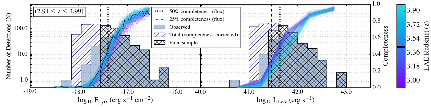
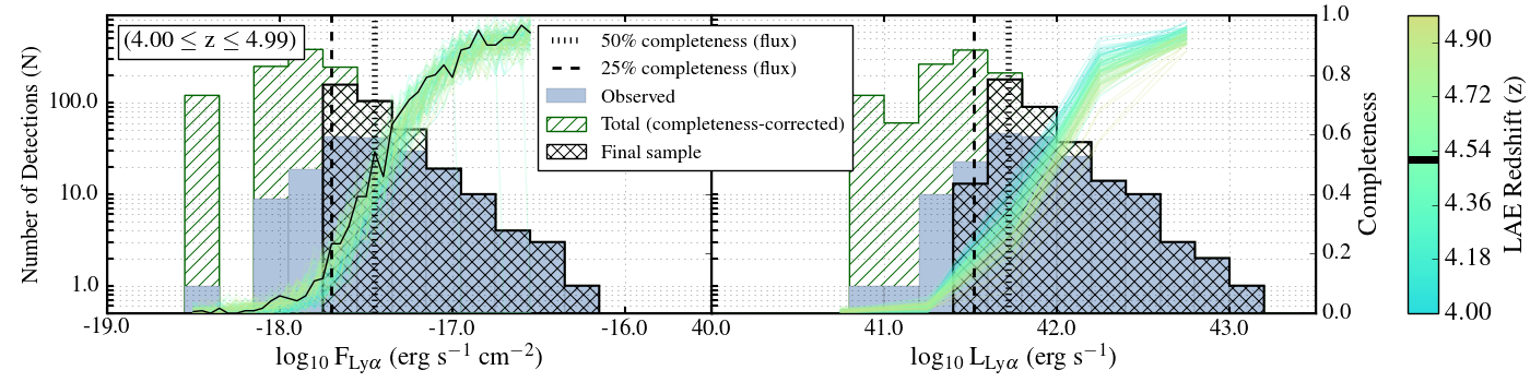
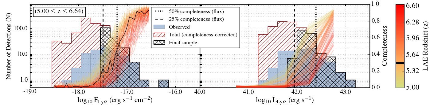
Fig. 7
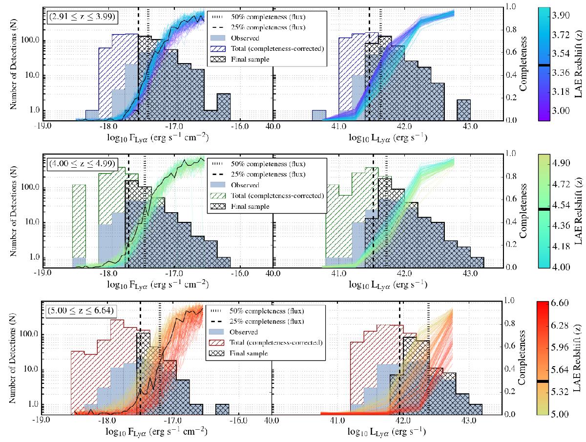
Flux and log-luminosity distributions of objects from the mosaic in three broad redshift bins at 2.91 ≤ z< 4.00, 4.00 ≤ z ≤ 4.99 and 5.00 ≤ z< 6.64. In each panel we show the total distribution of objects (including fakes created and added to the sample through the process described in Sect. 5.2) in a coloured hatched histogram. We overlay the distribution of observed objects in filled blue bars. The final samples, curtailed at the 25% completeness limit in flux (Δ f = 0.05) for the median redshift of objects in the redshift bin is overplotted in a bold cross-hatched black histogram. Overlaid on each panel are the completeness curves as a function of flux (or log luminosity) at each redshift (Δ z = 0.01) falling within the bin. Each redshift is given by a different coloured line according to the colour-map shown in the colour bar, and the curve at the median redshift of the bin is emphasized in black. The median redshift of the bin is also given by a black line on the colour bar.
Current usage metrics show cumulative count of Article Views (full-text article views including HTML views, PDF and ePub downloads, according to the available data) and Abstracts Views on Vision4Press platform.
Data correspond to usage on the plateform after 2015. The current usage metrics is available 48-96 hours after online publication and is updated daily on week days.
Initial download of the metrics may take a while.