© ESO, 2017

1. Introduction

It is generally believed that the plasma density decreases with height in the quiet Sun (see, e.g. Melrose 1980). However, some regions are more clearly visible than others in the solar atmosphere possibly due to localised heating and non-uniform plasma blobs present in these regions. It has been difficult to determine density stratification in such localised regions of the solar corona. In particular, the visible oscillating coronal loops are clearly illuminated against the surroundings in the Sun’s corona and it is generally believed that the plasma density along the field lines is denser compared to its surroundings in these loops. However, this really depends on the observing wavelength. Coronal extreme UV (EUV) wavelengths can cause cooler loops to appear dark compared to the material which surrounds them, and in certain EUV wavelengths, seemingly bright loops may be of lower density. The precise nature of the density stratification is, however, difficult to determine observationally, and multiple wavelength analysis is often necessary (e.g. Aschwanden 2005).

Some coronal loops have been seen to oscillate near regions of flaring events (Ashwanden et al. 1999; Nakariakov & Ofman 2001; Schrijver et al. 2002; Verwichte et al. 2004; Jain et al. 2014). Their intensity variations have been studied with the aim to determine magnetic field strength and density contrast in such oscillating loops (e.g. Nakariakov et al. 1999; Verwichte et al. 2004). An important observable of the oscillating loops is their periodicity (or the eigenfrequency of the trapped modes of oscillations) which are compared with the periodicities from an empirical model. These empirical models are crucial as the density and magnetic field strengths of the observed loops are then indirectly estimated from the models.

There have been many studies in the past that relate the oscillations of the coronal loops to the oscillations of a cavity in one-dimensional (1D) wave cavity models (Edwin & Roberts 1983; Goossens et al. 2002; Nakariakov & Verwichte 2005; Andries et al. 2009). A three-dimensional (3D) magnetohydrodynamic (MHD) model with dipole magnetic field in an isothermal condition was studied by Ofman et al. (2015) to explain vertical transverse oscillation (see also Liu & Ofman 2014). The authors conclude that the results of their stratified model are similar to a magnetic arcade without gravity. Recently strong evidence of multiple loops oscillating in a magnetic arcade has been reported by Jain et al. (2015) and Li et al. (2017), using AIA images (see, also, Verwichte et al. 2009, for TRACE data). Such observations undeniably require a new approach and investigation of wave cavities in multi-dimensional waveguides. In this context, Hindman & Jain (2014) explored the importance of fast MHD wave propagation in 2D and 3D waveguides (see Hindman & Jain 2015). Hindman & Jain (2014) argue that since the low-plasma-beta of the solar corona indicates a magnetically dominated environment, the eruptive events such as flares can easily stimulate and transmit fast MHD waves across the field lines of a coronal arcade. They first investigated the importance of fast MHD waves for a 2D waveguide and computed a continuous power spectrum due to fast wave propagation at an angle to the magnetic field direction for a driven problem. The interference between the waves travelling down the waveguides results in a rich power spectrum from which the dominant period and wavenumber information can be obtained. This enables an understanding of the type of oscillations, the waveguide, density and magnetic field stratification of the coronal loops in greater detail. Their work also emphasised the importance of magnetic pressure and magnetic tension forces in the corona as opposed to simply magnetic tension, the only restoring force in 1D wave-cavity models.

Recently, Hindman & Jain (2015) considered a 3D waveguide consisting of a two-shell model of coronal loop structure in a cylindrical magnetic arcade. They investigated the fast MHD wave propagation for such a model in which the axial direction is invariant and the waves are trapped in radial and azimuthal direction. This study explains, for the first time, how the coupling of axial and radial modes can be attributed to the different lines-of-sight observation of an oscillating loop, resulting in vertically and horizontally polarised oscillations and how such an elliptical polarisation varies with height in a loop. The Hindman & Jain (2015) model has been promising for our understanding of the coupling of radial and axial velocities in a 3D waveguide, although the model interface, which represents the region where the observed oscillations are supposed to reside, is a very thin layer of a sharp density discontinuity. It was clearly discussed by Goossens et al. (2002) that when a sharp discontinuous density is replaced by a continuous smooth density variation, it gives rise to quasi-modes which allow classic kink mode oscillations to be resonantly damped by quasi-modes (see also Ruderman & Roberts 2002). We defer the studies of quasi-modes for future work, and instead focus on studying the effect of a discontinuous transition of density on the fast discrete eigenmodes and eigenfunctions.

In this paper, we extend the two-shell model of Hindman & Jain (2015) by incorporating a middle shell of inhomogeneous density between the two shells to investigate whether a small variation in density structure alters the fast mode eigenfunctions or not. The middle shell represents the situation where an oscillating loop has maximum amplitude of oscillation in a region of enhanced or suppressed density compared to its immediate surroundings. We refer to this as a three-shell model. We first derive a dispersion relation relating the eigenfrequencies and wavenumbers and then solve it for various relative amplitudes of Alfvén speeds in the three shells. We compare the resulting propagation diagrams of eigenfrequencies for two-shell and three-shell models. We also compute the corresponding eigenfunctions to study various polarisations of the oscillating loop.

2. The model and governing equation

Following Hindman & Jain (2015), we consider the coronal loop structure as a half-cylindrical waveguide. We employ a model in cylindrical coordinates, that is (r,θ,y), and assume that the azimuthal range is such that θ lies between 0 and π, and assume the footpoints anchored in the photosphere.

In this regime, we assume a potential magnetic field of the form 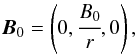$\begin{array}{ccc}{{B}}_{\mathrm{0}}\mathrm{=}\left(\mathrm{0}\mathit{,}\frac{{\mathit{B}}_{\mathrm{0}}}{\mathit{r}}\mathit{,}\mathrm{0}\right)\mathit{,}& & \end{array}$(1)in a low plasma-beta atmosphere, with negligible gravity effects. The equilibrium atmosphere is considered to be at rest.

Such a profile has been previously studied by many (e.g. Carrion 1988; Verwichte et al. 2006); however, none of these studies considered propagation in the axial direction perpendicular to the equilibrium magnetic field (i.e. in the y-direction), resulting in coupled radial and axial motion.

We also note that a more general magnetic field with B = (0,B_θ,B_z) has been considered for MHD waves in 1D straight cylindrical plasmas (Appert et al. 1974; Sakurai et al. 1991; Khongorova et al. 2012). However, in the current study we focus on propagation in 3D waveguide (see also, Hindman & Jain 2015) in cylindrical arcades with a middle shell of varying thickness. We consider fast mode propagation in axial direction (k ≠ 0) and show how the coupling of radial and axial velocities leads to mixed horizontal and vertical polarisations.

The corresponding linearised momentum equation is thus 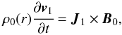${\mathit{\rho }}_{\mathrm{0}}\mathrm{\left(}\mathit{r}\mathrm{\right)}\frac{\mathit{\partial }{{v}}_{\mathrm{1}}}{\mathit{\partial t}}\mathrm{=}{{J}}_{\mathrm{1}}\mathrm{\times }{{B}}_{\mathrm{0}}\mathit{,}$(2)where subscript 0 denotes a background quantity, and subscript 1 a perturbed quantity. Here, J₁ is the perturbed current density.

Considering Fourier analysis of perturbed quantities in the form sin(mθ)e^ikye^{− iωt}, we derive the perturbed axial and radial velocities (see also Hindman & Jain 2015): 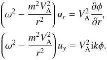$\begin{array}{ccc}\left({\mathit{\omega }}^{\mathrm{2}}\mathrm{-}\frac{{\mathit{m}}^{\mathrm{2}}{\mathit{V}}_{\mathrm{A}}^{\mathrm{2}}}{{\mathit{r}}^{\mathrm{2}}}\right){\mathit{u}}_{\mathit{r}}\mathrm{=}{\mathit{V}}_{\mathrm{A}}^{\mathrm{2}}\frac{\mathit{\partial \phi }}{\mathit{\partial r}}\mathit{,}& & \\ \left({\mathit{\omega }}^{\mathrm{2}}\mathrm{-}\frac{{\mathit{m}}^{\mathrm{2}}{\mathit{V}}_{\mathrm{A}}^{\mathrm{2}}}{{\mathit{r}}^{\mathrm{2}}}\right){\mathit{u}}_{\mathit{y}}\mathrm{=}{\mathit{V}}_{\mathrm{A}}^{\mathrm{2}}\mathrm{i}\mathit{k\phi }\mathit{.}& & \end{array}$(3)Here, V_A = V_A(r) is the Alfvén speed, and the function, 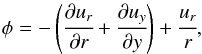$\begin{array}{ccc}\mathit{\phi }\mathrm{=}\mathrm{-}\left(\frac{\mathit{\partial }{\mathit{u}}_{\mathit{r}}}{\mathit{\partial r}}\mathrm{+}\frac{\mathit{\partial }{\mathit{u}}_{\mathit{y}}}{\mathit{\partial y}}\right)\mathrm{+}\frac{{\mathit{u}}_{\mathit{r}}}{\mathit{r}}\mathit{,}& & \end{array}$(4)is related to the temporal variation of the magnetic pressure.

Combining Eqs. (3) and (4) yields the governing equation $\begin{array}{ccc}{\mathit{\phi }}^{\mathrm{\prime \prime }}\mathrm{-}\left[\frac{\mathrm{1}}{\mathit{r}}\mathrm{+}\frac{\mathrm{1}}{{\mathrm{\Omega }}^{\mathrm{2}}}\frac{\mathrm{d}\mathrm{\left(}{\mathrm{\Omega }}^{\mathrm{2}}\mathrm{\right)}}{\mathrm{d}\mathit{r}}\right]{\mathit{\phi }}^{\mathrm{\prime }}\mathrm{+}\mathrm{(}{\mathrm{\Omega }}^{\mathrm{2}}\mathrm{-}{\mathit{k}}^{\mathrm{2}}\mathrm{)}\mathit{\phi }\mathrm{=}\mathrm{0}\mathit{,}& & \end{array}$(5)where ${\mathrm{\Omega }}^{\mathrm{2}}\mathrm{=}\frac{{\mathit{\omega }}^{\mathrm{2}}}{{\mathit{V}}_{\mathrm{A}}^{\mathrm{2}}}\mathrm{-}\frac{{\mathit{m}}^{\mathrm{2}}}{{\mathit{r}}^{\mathrm{2}}}\mathrm{·}$ Hindman & Jain (2015) solved this governing equation for an analytical model comprising two shells separated by an interface in the radial direction. In their model, density decreases radially as r^-4 in both shells, with a discontinuity at the interface. For such a density profile, the Alfvén speed V_A(r) ∝ r² in each shell and the governing equation is simplified considerably with solutions in terms of modified Bessel functions I and K. Although mathematically tractable, the Hindman & Jain (2015) model is only applicable if the oscillating coronal loops reside in a thin shell at the interface of a dense plasma overlying an evacuated cavity. It is quite possible that many field lines close to one another can oscillate simultaneously in a wider region of smoothly varying density (instead of an interface with sharp density discontinuity) in the solar corona. A natural extension of this two-shell model, therefore, is with the inclusion of a middle shell of finite width near the interface. This is what is considered in the following sections.

The limit as r → 0 must first be addressed, since at r = 0 the magnitude of the magnetic field in (1) becomes infinitely large. Consider the two-shell model as in Hindman & Jain (2015), such that the Alfvén speed profile is $\begin{array}{ccc}{\mathit{V}}_{\mathrm{A}}\mathrm{\left(}\mathit{r}\mathrm{\right)}\mathrm{=}\{\begin{array}{c}\\ & \\ & \end{array}& & \end{array}$(6)in the limit where b → 0. The resulting eigenfunctions of the governing Eq. (5) for the profile (6) yields $\begin{array}{ccc}\mathit{\phi }\mathrm{=}\{\begin{array}{c}\\ & \\ & \end{array}& & \end{array}$(7)where $\begin{array}{ccc}{\mathit{\nu }}^{\mathrm{2}}\mathrm{=}\{\begin{array}{c}\\ & \\ & \end{array}& & \end{array}$(8)Continuity of eigenfunctions φ and the radial velocity u_r at r = r₀, and the condition φ(b) = 0 with evanescent solutions as r → ∞ produces the dispersion relation $\begin{array}{ccc}{\mathit{\nu }}_{\mathrm{1}}^{\mathrm{2}}\frac{{\mathit{I}}_{{\mathit{\nu }}_{\mathrm{0}}}^{\mathrm{\prime }}\mathrm{\left(}\mathit{k}{\mathit{r}}_{\mathrm{0}}\mathrm{\right)}}{\left[{\mathit{I}}_{{\mathit{\nu }}_{\mathrm{0}}}\mathrm{\left(}\mathit{k}{\mathit{r}}_{\mathrm{0}}\mathrm{\right)}\mathrm{-}\frac{{\mathit{I}}_{{\mathit{\nu }}_{\mathrm{0}}}\mathrm{\left(}\mathit{kb}\mathrm{\right)}}{{\mathit{K}}_{{\mathit{\nu }}_{\mathrm{0}}}\mathrm{\left(}\mathit{kb}\mathrm{\right)}}\right]}\mathrm{=}{\mathit{\nu }}_{\mathrm{0}}^{\mathrm{2}}\frac{{\mathit{K}}^{\mathrm{\prime }}{\mathit{\nu }}_{\mathrm{1}}\mathrm{\left(}\mathit{k}{\mathit{r}}_{\mathrm{0}}\mathrm{\right)}}{{\mathit{K}}_{{\mathit{\nu }}_{\mathrm{1}}}\mathrm{\left(}\mathit{k}{\mathit{r}}_{\mathrm{0}}\mathrm{\right)}}\mathrm{·}& & \end{array}$(9)Figure 1 shows the resulting eigenvalues obtained by solving Eq. (9) with solid lines for kb = 0.01 and kb = 0.5. For comparison, we also plot the eigenvalues of the two-shell model of Hindman & Hain (2015), where kb ≡ 0. We note that in the left panel, where kb = 0.01, the curves are indistinguishable from one another for all wavenumbers (kr₀) considered here. This is because the ratio $\frac{{\mathit{I}}_{{\mathit{\nu }}_{\mathrm{0}}}\mathrm{\left(}\mathit{kb}\mathrm{\right)}}{{\mathit{K}}_{{\mathit{\nu }}_{\mathrm{0}}}\mathrm{\left(}\mathit{kb}\mathrm{\right)}}$ is very small for kb ≪ 1. Thus, if kb ≪ 1, the magnetic field profile (see Eq. (1)) is reasonable, and we will consider the model arcades to be valid in 0 <r< ∞. This is justifiable as the eigenfunctions are evanescent for r ≪ r₀ and r ≫ r₀ + a.

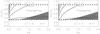Fig. 1 Propagation diagram for the eigenfrequencies $\frac{\mathit{\omega }{\mathit{r}}_{\mathrm{0}}}{{\mathit{V}}_{\mathrm{0}}}$ against the wavenumber kr0, for the ratio$\frac{{\mathit{V}}_{\mathrm{1}}^{\mathrm{2}}}{{\mathit{V}}_{\mathrm{0}}^{\mathrm{2}}}\mathrm{=}\mathrm{0.1}$, and m = 1, for kb = 0.01 (left) and kb = 0.5 (right).

3. Three-shell profile

We consider the Alfvén speed V_A(r) in each shell as follows: 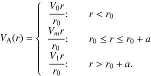$\begin{array}{ccc}{\mathit{V}}_{\mathrm{A}}\mathrm{\left(}\mathit{r}\mathrm{\right)}\mathrm{=}\{\begin{array}{c}\\ & \\ & \\ & \end{array}& & \end{array}$(10)The corresponding densities ρ(r) in the shells are: $\begin{array}{ccc}\mathit{\rho }\mathrm{\left(}\mathit{r}\mathrm{\right)}\mathrm{=}\{\begin{array}{c}\\ & \\ & \\ & \end{array}& & \end{array}$(11)We note that there are two interfaces, r = r₀ and r = r₀ + a. An Alfvén speed profile such as the one shown in Eq. (10) enables two reasonable scenarios for the coronal loop densities. The first one is where V₁<V₀: thus, V₁<V_m<V₀, V₁<V₀<V_m or V_m<V₁<V₀. We will refer to this as the “piecewise linear I” model. The second one is where V₀ = V₁ and V_0,1>V_m, such that the middle shell is denser than its surroundings. We refer to this as the “piecewise linear II” model. We discuss results for each model after solving the governing equation.

Using the Alfvén speed profiles (10), the governing Eq. (5) reduces to 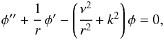$\begin{array}{ccc}{\mathit{\phi }}^{\mathrm{\prime \prime }}\mathrm{+}\frac{\mathrm{1}}{\mathit{r}}{\mathit{\phi }}^{\mathrm{\prime }}\mathrm{-}\left(\frac{{\mathit{\nu }}^{\mathrm{2}}}{{\mathit{r}}^{\mathrm{2}}}\mathrm{+}{\mathit{k}}^{\mathrm{2}}\right)\mathit{\phi }\mathrm{=}\mathrm{0}\mathit{,}& & \end{array}$(12)with 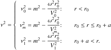$\begin{array}{ccc}{\mathit{\nu }}^{\mathrm{2}}\mathrm{=}\{\begin{array}{c}\\ & \\ & \\ & \end{array}& & \end{array}$(13)The solution of Eq. (12) takes the form of the modified Bessel functions I, K and L as defined in Dunster et al. (1990). For ${\mathit{\nu }}_{\mathit{m}}^{\mathrm{2}}\mathit{>}\mathrm{0}$, Eq. (12) yields 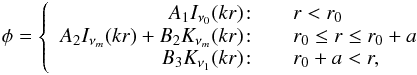$\begin{array}{ccc}\mathit{\phi }\mathrm{=}\{\begin{array}{c}\\ & \\ & \\ & \end{array}& & \end{array}$(14)where we ensure boundedness as r → 0 and r → ∞.

Similarly, for ${\mathit{\nu }}_{\mathit{m}}^{\mathrm{2}}\mathit{<}\mathrm{0}$, the solution becomes $\begin{array}{ccc}\mathit{\phi }\mathrm{=}\{\begin{array}{c}\\ & \\ & \\ & \end{array}& & \end{array}$(15)where ${\mathit{L}}_{{\mathit{\nu }}_{\mathit{m}}}\mathrm{\left(}\mathit{kr}\mathrm{\right)}\mathrm{=}\frac{\mathit{\pi i}}{\mathrm{2}\sin \mathrm{\left(}{\mathit{\nu }}_{\mathit{m}}\mathit{\pi }\mathrm{\right)}}\left\{{\mathit{I}}_{{\mathit{\nu }}_{\mathit{m}}}\mathrm{\left(}\mathit{kr}\mathrm{\right)}\mathrm{+}{\mathit{I}}_{\mathrm{-}{\mathit{\nu }}_{\mathit{m}}}\mathrm{\left(}\mathit{kr}\mathrm{\right)}\right\}\mathit{,}$(16)as defined in Dunster (1990).

The choice of ${\mathit{\nu }}_{\mathrm{0}}^{\mathrm{2}}\mathit{>}\mathrm{0}$ is implied, since otherwise the modified Bessel function I becomes complex and unbounded at the origin. The choice of parity for ${\mathit{\nu }}_{\mathrm{1}}^{\mathrm{2}}$ becomes more clear when considering the propagation diagrams, shown in Sect. 4.

4. Results

4.1. Dispersion relation

Continuity of eigenfunctions and the radial velocity, at r₀ and r₀ + a, yields the dispersion relation. For the case where ${\mathit{\nu }}_{\mathit{m}}^{\mathrm{2}}\mathit{>}\mathrm{0}$ in Eq. (14), it takes the form 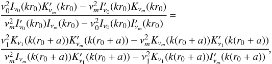$\begin{array}{ccc}& & \frac{{\mathit{\nu }}_{\mathrm{0}}^{\mathrm{2}}{\mathit{I}}_{{\mathit{\nu }}_{\mathrm{0}}}\mathrm{\left(}\mathit{k}{\mathit{r}}_{\mathrm{0}}\mathrm{\right)}{\mathit{K}}_{{\mathit{\nu }}_{\mathit{m}}}^{\mathrm{\prime }}\mathrm{\left(}\mathit{k}{\mathit{r}}_{\mathrm{0}}\mathrm{\right)}\mathrm{-}{\mathit{\nu }}_{\mathit{m}}^{\mathrm{2}}{\mathit{I}}_{{\mathit{\nu }}_{\mathrm{0}}}^{\mathrm{\prime }}\mathrm{\left(}\mathit{k}{\mathit{r}}_{\mathrm{0}}\mathrm{\right)}{\mathit{K}}_{{\mathit{\nu }}_{\mathit{m}}}\mathrm{\left(}\mathit{k}{\mathit{r}}_{\mathrm{0}}\mathrm{\right)}}{{\mathit{\nu }}_{\mathit{m}}^{\mathrm{2}}{\mathit{I}}_{{\mathit{\nu }}_{\mathrm{0}}}^{\mathrm{\prime }}\mathrm{\left(}\mathit{k}{\mathit{r}}_{\mathrm{0}}\mathrm{\right)}{\mathit{I}}_{{\mathit{\nu }}_{\mathit{m}}}\mathrm{\left(}\mathit{k}{\mathit{r}}_{\mathrm{0}}\mathrm{\right)}\mathrm{-}{\mathit{\nu }}_{\mathrm{0}}^{\mathrm{2}}{\mathit{I}}_{{\mathit{\nu }}_{\mathrm{0}}}\mathrm{\left(}\mathit{k}{\mathit{r}}_{\mathrm{0}}\mathrm{\right)}{\mathit{I}}_{{\mathit{\nu }}_{\mathit{m}}}^{\mathrm{\prime }}\mathrm{\left(}\mathit{k}{\mathit{r}}_{\mathrm{0}}\mathrm{\right)}}\mathrm{=}\\ & & \frac{{\mathit{\nu }}_{\mathrm{1}}^{\mathrm{2}}{\mathit{K}}_{{\mathit{\nu }}_{\mathrm{1}}}\mathrm{\left(}\mathit{k}\mathrm{\right(}{\mathit{r}}_{\mathrm{0}}\mathrm{+}\mathit{a}\mathrm{\left)}\mathrm{\right)}{\mathit{K}}_{{\mathit{\nu }}_{\mathit{m}}}^{\mathrm{\prime }}\mathrm{\left(}\mathit{k}\mathrm{\right(}{\mathit{r}}_{\mathrm{0}}\mathrm{+}\mathit{a}\mathrm{\left)}\mathrm{\right)}\mathrm{-}{\mathit{\nu }}_{\mathit{m}}^{\mathrm{2}}{\mathit{K}}_{{\mathit{\nu }}_{\mathit{m}}}\mathrm{\left(}\mathit{k}\mathrm{\right(}{\mathit{r}}_{\mathrm{0}}\mathrm{+}\mathit{a}\mathrm{\left)}\mathrm{\right)}{\mathit{K}}_{{\mathit{\nu }}_{\mathrm{1}}}^{\mathrm{\prime }}\mathrm{\left(}\mathit{k}\mathrm{\right(}{\mathit{r}}_{\mathrm{0}}\mathrm{+}\mathit{a}\mathrm{\left)}\mathrm{\right)}}{{\mathit{\nu }}_{\mathit{m}}^{\mathrm{2}}{\mathit{I}}_{{\mathit{\nu }}_{\mathit{m}}}\mathrm{\left(}\mathit{k}\mathrm{\right(}{\mathit{r}}_{\mathrm{0}}\mathrm{+}\mathit{a}\mathrm{\left)}\mathrm{\right)}{\mathit{K}}_{{\mathit{\nu }}_{\mathrm{1}}}^{\mathrm{\prime }}\mathrm{\left(}\mathit{k}\mathrm{\right(}{\mathit{r}}_{\mathrm{0}}\mathrm{+}\mathit{a}\mathrm{\left)}\mathrm{\right)}\mathrm{-}{\mathit{\nu }}_{\mathrm{1}}^{\mathrm{2}}{\mathit{K}}_{{\mathit{\nu }}_{\mathrm{1}}}\mathrm{\left(}\mathit{k}\mathrm{\right(}{\mathit{r}}_{\mathrm{0}}\mathrm{+}\mathit{a}\mathrm{\left)}\mathrm{\right)}{\mathit{I}}_{{\mathit{\nu }}_{\mathit{m}}}^{\mathrm{\prime }}\mathrm{\left(}\mathit{k}\mathrm{\right(}{\mathit{r}}_{\mathrm{0}}\mathrm{+}\mathit{a}\mathrm{\left)}\mathrm{\right)}}\mathit{,}\end{array}$(17)and when ${\mathit{\nu }}_{\mathit{m}}^{\mathrm{2}}\mathit{<}\mathrm{0}$ (see Eq. (15)), the L_νm modified Bessel function is used in place of I_νm.

Fig. 2 The non-dimensionalised Alfvén speed $\frac{{\mathit{V}}_{\mathrm{A}}}{{\mathit{V}}_{\mathrm{0}}}$ against the wavenumber kr, for a) ${\mathit{\nu }}_{\mathit{m}}^{\mathrm{2}}\mathit{>}\mathrm{0}$: $\frac{{\mathit{V}}_{\mathit{m}}^{\mathrm{2}}}{{\mathit{V}}_{\mathrm{0}}^{\mathrm{2}}}\mathrm{=}\mathrm{0.5}$ (top panel), $\frac{{\mathit{V}}_{\mathit{m}}^{\mathrm{2}}}{{\mathit{V}}_{\mathrm{0}}^{\mathrm{2}}}\mathrm{=}\mathrm{2}$ (middle panel), and b) ${\mathit{\nu }}_{\mathit{m}}^{\mathrm{2}}\mathit{<}\mathrm{0}$: $\frac{{\mathit{V}}_{\mathit{m}}^{\mathrm{2}}}{{\mathit{V}}_{\mathrm{0}}^{\mathrm{2}}}\mathrm{=}\mathrm{0.05}$ (bottom panel). In all cases, $\frac{{\mathit{V}}_{\mathrm{1}}^{\mathrm{2}}}{{\mathit{V}}_{\mathrm{0}}^{\mathrm{2}}}\mathrm{=}\mathrm{0.1}$ and kr0 = 0.2, for ka = 0.1 (left) and ka = 0.5 (right).

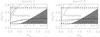Fig. 3 Case I: ${\mathit{\nu }}_{\mathit{m}}^{\mathrm{2}}\mathit{>}\mathrm{0}$. Propagation diagram for the eigenfrequencies $\frac{\mathit{\omega }{\mathit{r}}_{\mathrm{0}}}{{\mathit{V}}_{\mathrm{0}}}$ against the wavenumber kr0, for the ratios $\frac{{\mathit{V}}_{\mathit{m}}^{\mathrm{2}}}{{\mathit{V}}_{\mathrm{0}}^{\mathrm{2}}}\mathrm{=}\mathrm{0.5}$ and $\frac{{\mathit{V}}_{\mathrm{1}}^{\mathrm{2}}}{{\mathit{V}}_{\mathrm{0}}^{\mathrm{2}}}\mathrm{=}\mathrm{0.1}$, and m = 1, for ka = 0.1 (left) and ka = 0.5 (right).

Solving the dispersion relation for the eigenfrequencies $\frac{\mathit{\omega }{\mathit{r}}_{\mathrm{0}}}{{\mathit{V}}_{\mathrm{0}}}$ and wavenumber kr₀ allows us to examine the propagating and evanescent regions. The wavenumber kr₀ can be considered as the non-dimensionalised location of the first interface, between the inner cavity and the middle layer, and the thickness of the middle shell is represented by the non-dimensionalised quantity ka. Throughout, the propagation diagrams show the solid curves as obtained from the three-shell model and the dashed-dot curves as obtained from the two-shell model.

4.2. The piecewise linear I model

In this model, we consider two cases: ${\mathit{\nu }}_{\mathit{m}}^{\mathrm{2}}\mathit{>}\mathrm{0}$ and ${\mathit{\nu }}_{\mathit{m}}^{\mathrm{2}}\mathit{<}\mathrm{0}$. Taking the ratio $\frac{{\mathit{V}}_{\mathrm{1}}^{\mathrm{2}}}{{\mathit{V}}_{\mathrm{0}}^{\mathrm{2}}}\mathrm{=}\mathrm{0.1}$ and the location of the first interface to be kr₀ = 0.2, the plots of the non-dimensionalised Alfvén speed against the wavenumber kr, are shown in Fig. 2 for thicknesses ka = 0.1 (left) and ka = 0.5 (right). In the top panel, we have assumed $\frac{{\mathit{V}}_{\mathit{m}}^{\mathrm{2}}}{{\mathit{V}}_{\mathrm{0}}^{\mathrm{2}}}\mathrm{=}\mathrm{0.5}$, in the middle panel $\frac{{\mathit{V}}_{\mathit{m}}^{\mathrm{2}}}{{\mathit{V}}_{\mathrm{0}}^{\mathrm{2}}}\mathrm{=}\mathrm{2}$, and in the bottom panel $\frac{{\mathit{V}}_{\mathit{m}}^{\mathrm{2}}}{{\mathit{V}}_{\mathrm{0}}^{\mathrm{2}}}\mathrm{=}\mathrm{0.05}$.

4.2.1. Case I: ${\mathit{\nu }}_{\mathit{m}}^{\mathrm{2}}\mathit{>}\mathrm{0}$

First consider the case where V₁<V_m<V₀. We solve the dispersion relation (17) for the Alfvén speeds shown in Fig. 2 and plot the propagation diagram in Fig. 3, for azimuthal order m = 1. The upper and lower dashed lines are governed by the parity of ${\mathit{\nu }}_{\mathit{m}}^{\mathrm{2}}$ and ${\mathit{\nu }}_{\mathrm{1}}^{\mathrm{2}}$ – in this case; for there to be propagating solutions, we take ${\mathit{\nu }}_{\mathit{m}}^{\mathrm{2}}\mathit{>}\mathrm{0}$ and we must take ${\mathit{\nu }}_{\mathrm{1}}^{\mathrm{2}}\mathit{<}\mathrm{0}$, to ensure boundedness of eigenfunctions as r → ∞. The grey area indicates the evanescent region, and the white area the propagating region, separated by a curve representing the cut-off frequency, above which waves propagate, and below which they are evanescent. The solid curves indicate the modes for the three-shell model. We also consider the two-shell model (see Hindman & Jain 2015) and solve the corresponding dispersion relation 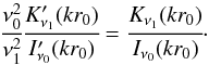$\frac{{\mathit{\nu }}_{\mathrm{0}}^{\mathrm{2}}}{{\mathit{\nu }}_{\mathrm{1}}^{\mathrm{2}}}\frac{{\mathit{K}}_{{\mathit{\nu }}_{\mathrm{1}}}^{\mathrm{\prime }}\mathrm{\left(}\mathit{k}{\mathit{r}}_{\mathrm{0}}\mathrm{\right)}}{{\mathit{I}}_{{\mathit{\nu }}_{\mathrm{0}}}^{\mathrm{\prime }}\mathrm{\left(}\mathit{k}{\mathit{r}}_{\mathrm{0}}\mathrm{\right)}}\mathrm{=}\frac{{\mathit{K}}_{{\mathit{\nu }}_{\mathrm{1}}}\mathrm{\left(}\mathit{k}{\mathit{r}}_{\mathrm{0}}\mathrm{\right)}}{{\mathit{I}}_{{\mathit{\nu }}_{\mathrm{0}}}\mathrm{\left(}\mathit{k}{\mathit{r}}_{\mathrm{0}}\mathrm{\right)}}\mathrm{·}$(18)The curves for the two-shell model are overplotted in Fig. 3 as dash-dot lines.

We note that the n = 0 mode exists for both the two-shell (dash-dot) and three-shell (solid) models. It also changes the propagating behaviour to evanescence for large values of kr₀ in both models. However, as the thickness of the middle layer increases in the three-shell model, the absence of the higher order radial modes is noticeable. The n = 1 mode is present for ka = 0.1 (left panel) but is suppressed in the right panel for ka = 0.5. Recall that ka should be exactly zero for the dash-dot curves and that is why the dash-dot and solid curves do not overlap here. The non-dimensionalised eigenfrequencies (obtained for kr₀ = 0.1 in the two-shell model) now corresponds to kr₀ = 0 and ka = 0.1. To further study the nature of the propagating solutions, we examine the eigenfunctions.

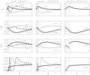Fig. 4 Case I: ${\mathit{\nu }}_{\mathit{m}}^{\mathrm{2}}\mathit{>}\mathrm{0}$. The eigenfunction, φ, normalised radial and axial velocities, ur and uy and polarisation fraction, f, against the wavenumber kr, for the ratios $\frac{{\mathit{V}}_{\mathit{m}}^{\mathrm{2}}}{{\mathit{V}}_{\mathrm{0}}^{\mathrm{2}}}\mathrm{=}\mathrm{1}$ and $\frac{{\mathit{V}}_{\mathrm{1}}^{\mathrm{2}}}{{\mathit{V}}_{\mathrm{0}}^{\mathrm{2}}}\mathrm{=}\mathrm{0.1}$, kr0 = 0.2, and m = 1, for ka = 0 (left column). This is analogous to the two-shell case. The middle column and right column are for the cases $\frac{{\mathit{V}}_{\mathit{m}}^{\mathrm{2}}}{{\mathit{V}}_{\mathrm{0}}^{\mathrm{2}}}\mathrm{=}\mathrm{0.5}$ and $\frac{{\mathit{V}}_{\mathrm{1}}^{\mathrm{2}}}{{\mathit{V}}_{\mathrm{0}}^{\mathrm{2}}}\mathrm{=}\mathrm{0.1}$, with kr0 = 0.2, and m = 1, for ka = 0.1 and ka = 0.5, respectively. The curves are normalised with respect to the eigenfunctions, for comparison.

We once again set ka = 0 and $\frac{{\mathit{V}}_{\mathit{m}}^{\mathrm{2}}}{{\mathit{V}}_{\mathrm{0}}^{\mathrm{2}}}\mathrm{=}\mathrm{1}$ to reproduce the two-shell eigenfunctions studied in Hindman & Jain (2015), and compare with eigenfunctions for the three-shell model for $\frac{{\mathit{V}}_{\mathit{m}}^{\mathrm{2}}}{{\mathit{V}}_{\mathrm{0}}^{\mathrm{2}}}\ne \mathrm{1}$, ka ≠ 0. Thus, in Fig. 4, we plot the non-dimensionalised eigenfunctions φ, and the radial and axial velocities as a function of kr for three different values of ka. As expected from Fig. 3, not only are the higher-order modes absent in the middle and right panels, the peaks of the eigenmodes are now at the interface ka. This can be understood by the fact that it is as if the eigenfrequencies of the two-shell model are shifted from kr₀ to ka.

We also plot the polarisation fraction, f, defined as 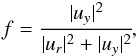$\begin{array}{ccc}\mathit{f}\mathrm{=}\frac{\mathrm{|}{\mathit{u}}_{\mathit{y}}{\mathrm{|}}^{\mathrm{2}}}{\mathrm{|}{\mathit{u}}_{\mathit{r}}{\mathrm{|}}^{\mathrm{2}}\mathrm{+}\mathrm{|}{\mathit{u}}_{\mathit{y}}{\mathrm{|}}^{\mathrm{2}}}\mathit{,}& & \end{array}$(19)to study what portion of radial and axial velocities contribute at each wavenumber.

The fraction yields a value of 0 if the motion of the wave is fully radial, and yields a value of 1 if the motion is fully axial. The n = 0 mode displays a mixture of axial and radial motion. Such elliptical polarisation can be seen even for ka ≠ 0, but the location of the peak value appears to be shifted based on the thickness of the middle shell. The polarisation fraction also changes with radial height in all cases.

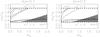Fig. 5 Same as Fig. 3, except for $\frac{{\mathit{V}}_{\mathit{m}}^{\mathrm{2}}}{{\mathit{V}}_{\mathrm{0}}^{\mathrm{2}}}\mathrm{=}\mathrm{2}$.

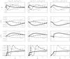Fig. 6 Same as Fig. 4, except $\frac{{\mathit{V}}_{\mathit{m}}^{\mathrm{2}}}{{\mathit{V}}_{\mathrm{0}}^{\mathrm{2}}}\mathrm{=}\mathrm{2}$.

Now, we consider the case where V₁<V₀<V_m. Solving the dispersion relation (17) for the Alfvén speeds in (10), the propagation diagrams shown in Fig. 5 are obtained. The upper boundary is now raised to where ${\mathit{\nu }}_{\mathrm{0}}^{\mathrm{2}}$ will allow real eigenfrequencies. As a result, for ka = 0.1, the n = 2 curve is no longer suppressed, and for ka = 0.5, the n = 1 curve now exists. Similar to Fig. 3, the solid curves do not overlap with the dash-dot curves.

We compare the eigenfunctions in Fig. 6 in the same format as in Fig. 4. In the top panel, we note that the peaks are shifted to the interface at ka, and the n = 2 mode now exists for ka = 0.1, but is suppressed for ka = 0.5. The middle two panels once again indicate the axial and radial motion, as a function of kr. For the polarisation fraction, it is clear that the peak values are once again shifted relative to the position of the second interface, with elliptical motion present for large wavenumbers. Despite the shift, the polarisation fraction of n = 0 remains mostly unchanged.

It is interesting to note from Figs. 3 and 5 that if the middle shell is thin (e.g. ka = 0.1) and is less dense than the inner cavity (where r<r₀), and the eigenmodes and their behaviour are similar to the two-shell eigenfunctions. However, if the middle shell is denser than the inner cavity, the higher radial modes (n ≥ 2) do not exist.

4.2.2. Case II: ${\mathit{\nu }}_{\mathit{m}}^{\mathrm{2}}\mathit{<}\mathrm{0}$

For V₁<V_m<V₀ and V_m<V₁<V₀, we can also consider the case where ${\mathit{\nu }}_{\mathit{m}}^{\mathrm{2}}\mathit{<}\mathrm{0}$. Solving the dispersion relation with L_νm in place of I_νm in Eq. (17), when V₁<V_m<V₀ , we obtain the eigenfrequencies $\frac{\mathit{\omega }{\mathit{r}}_{\mathrm{0}}}{{\mathit{V}}_{\mathrm{0}}}$ and wavenumber kr₀. The resulting propagation diagrams are shown in Fig. 7.

It is immediately apparent in Fig. 7 that the choice of ${\mathit{\nu }}_{\mathit{m}}^{\mathrm{2}}\mathit{<}\mathrm{0}$ has diminished the evanescent region that was previously shaded grey in Fig. 3. The change in parity of ${\mathit{\nu }}_{\mathit{m}}^{\mathrm{2}}$ means that the upper boundary is indicative of ${\mathit{\nu }}_{\mathrm{0}}^{\mathrm{2}}\mathit{>}\mathrm{0}$, and the lower boundary of ${\mathit{\nu }}_{\mathit{m}}^{\mathrm{2}}\mathit{<}\mathrm{0}$. The solid lines once again show the modes in the three-shell case, and the dash-dot the modes in the two-shell case. The n = 0 curve in both plots becomes almost parallel with the lower boundary, though the n = 0 curve in the ka = 0.1 now begins at a non-zero wavenumber, around 0.3, since, as for ${\mathit{\nu }}_{\mathit{m}}^{\mathrm{2}}\mathit{>}\mathrm{0}$, we have a non-zero interface at ka when kr₀ = 0. The n = 1 and n = 2 curves in both propagation diagrams are displaced significantly when compared with the corresponding modes in the two-shell case. In the bottom right of each plot is the line which divides the evanescent and propagating regions.

Examination of the eigenmodes, radial and axial velocities and polarisation fraction, in Fig. 8, for the ka = 0.1 case, in comparison to the two-shell case, indicates that only the n = 1 and n = 2 modes exist for kr₀ = 0.2. As expected for the ka = 0.5 case, only the n = 0 and n = 1 modes exist. The axial velocity for n = 0 shows quite unique behaviour in the middle shell. Once again, all modes exhibit evanescent behaviour below kr₀, and for large wavenumbers, kr.

Qualitatively, the radial velocities in the middle panel have the same behaviour after the second interface as they do beyond the interface in the corresponding plot to the left. However, the axial velocity of the n = 1 mode is enhanced in the middle layer for the ka = 0.1 case, resulting in mostly an axial motion in the polarisation fraction plot below. Once again, as in the two-shell case, the curves exhibit a mixture of axial and radial motions beyond the interface. In the right panel, the polarisation plot indicates that both the n = 0 and n = 1 modes exhibit a mixture of both radial and axial motion, particularly in the middle shell. For both ka = 0.1 and ka = 0.5, as the wavenumber becomes large the motion becomes almost equally radial and axial.

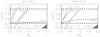Fig. 7 Case II: ${\mathit{\nu }}_{\mathit{m}}^{\mathrm{2}}\mathit{<}\mathrm{0}$. All parameters the same as in Fig. 4.

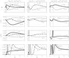Fig. 8 Case II: ${\mathit{\nu }}_{\mathit{m}}^{\mathrm{2}}\mathit{<}\mathrm{0}$. All parameters the same as in Fig. 4.

Now, consider the model where V_m<V₁<V₀. Figure 9 shows the propagation diagrams for this case. The lower boundary of permitted real eigenfrequencies is now imposed by the condition ${\mathit{\nu }}_{\mathrm{1}}^{\mathrm{2}}\mathit{<}\mathrm{0}$. Once again, the solid lines indicate the three-shell curves, and the dashed-dot lines the two-shell curves. Whilst there is suppression of some of the radial modes, at kr₀ = 0.2, the n = 2 mode still exists for both ka = 0.1 and ka = 0.5. Comparing the two thicknesses, we note that when the thickness of the middle shell increases, the number of modes increases. This is because, when ka becomes larger, it is as if we have only one interface at kr₀ = 0.2, and so waves are produced in a similar manner as in the two-shell model.

We find the eigenfunctions, radial and axial velocities and polarisation fraction, as before, and plot them in Fig. 10. It is clear that as the middle shell widens, more and more higher-order modes are present. The modes of higher radial orders are clearly visible in the middle shell for ka = 0.5.

The axial and radial motion shown in the middle panels is manifested in the polarisation plots on the bottom panel. For large wavenumbers, motion becomes a mixture of both radial and axial, though, in both plots, n = 1, n = 2 and (in the ka = 0.5 plot) n = 3 show elliptical motion initially after the first interface.

4.3. The piecewise linear II model

If coronal loops are, in fact, an augmentation of plasma which lies along the field-lines of a coronal arcade, then it logically follows that the density structure in the inner cavity would be the same just above and below the middle-shell. We thus consider ${\mathit{\nu }}_{\mathrm{1}}^{\mathrm{2}}\mathrm{=}{\mathit{\nu }}_{\mathrm{0}}^{\mathrm{2}}\mathit{>}\mathrm{0}$, with the Alfvén speed profile demonstrated in Fig 11. Hence, for real eigenfrequencies to exist, ${\mathit{\nu }}_{\mathit{m}}^{\mathrm{2}}\mathit{<}\mathrm{0}$ for V_m<V₀. We note that the case for V_m>V₀(=V₁) would correspond to a rarer middle shell surrounded by denser regions above and below it. Since coronal loops are believed to reside in a denser region, we do not consider this case.

Figure 12 shows the propagation diagram for $\frac{{\mathit{V}}_{\mathit{m}}^{\mathrm{2}}}{{\mathit{V}}_{\mathrm{0}}^{\mathrm{2}}}\mathrm{=}\mathrm{0.1}$ where we first notice that for the three-shell model (solid curves), the eigenfrequencies are lower than the two-shell model (dash-dot curves), for large kr. The second substantial curve, n = 1, asymptotes for large wavenumbers, as the n = 0 mode did for the piecewise linear I model. For ka = 0.1, there are only three modes in the propagating region, though one exists only for small wavenumbers. In the ka = 0.5 plot, there is still the existence of a mode close to the lower boundary, however the higher-radial-order modes take on much the same qualitative behaviour as in the piecewise linear I model. We note that, in the ka = 0.5 plot, both the n = 0 and n = 1 curves become evanescent modes for high wavenumbers.

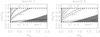Fig. 9 Same as Fig. 7, except $\frac{{\mathit{V}}_{\mathit{m}}^{\mathrm{2}}}{{\mathit{V}}_{\mathrm{0}}^{\mathrm{2}}}\mathrm{=}\mathrm{0.05}$.

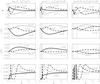Fig. 10 Same as Fig. 8, except $\frac{{\mathit{V}}_{\mathit{m}}^{\mathrm{2}}}{{\mathit{V}}_{\mathrm{0}}^{\mathrm{2}}}\mathrm{=}\mathrm{0.05}$.

Figure 13 shows the φ eigenfunction, radial and axial velocities, and polarisation fraction, as a function of kr. For ka = 0.5, we see that the eigenfunction for n = 0 (solid) and n = 1 (dotted) is evanescent in the middle shell, that is, between kr₀ and kr₀ + ka. The dashed line (n = 2) is a body mode in the middle region. Figure 13 also shows that the axial velocity peaks in the middle shell. Thus, as shown in the bottom panel, the polarisation is predominantly axial in the middle shell.

5. Discussion

The actual oscillating solar coronal loops reside in a magnetic arcade, which appear to be finite in length. There is inhomogeneity along the waveguide and in the direction transverse to the magnetic loops. In the current model, we assume that the scale-length of the inhomogeneity along the waveguide is much larger than the scale-length of the inhomogeneity across the height of the arcade and thus we ignore the inhomogeneity in the axial direction and consider the magnetic field and density varying in the radial direction.

Hindman & Jain (2015) considered the density to decrease with the height in a cylindrical loop separated at an interface. They found that fast waves can be trapped if the Alfvén speed increases with height. In the present work, we introduced a middle shell near the interface. We find that the behaviour of the fast MHD waves depend significantly on the density variation with height with localised eigenmodes absent if the density decreases slowly with height. However, if the density decreases rapidly with height, the fast MHD waves are naturally refracted back towards the photosphere, forming a cavity within which they are trapped. Such modes will have a discrete spectrum.

When ${\mathit{\nu }}_{\mathit{m}}^{\mathrm{2}}\mathit{<}\mathrm{0}$ (see Figs. 8 and 9), the three-shell model yields similar results for the larger middle-shell as the two-shell model. This is because, for large ka, the dispersion relation (17) reduces to the dispersion relation obtained for the two-shell model (see Eq. (18)). This can be understood as follows.

When the thickness of the middle shell increases,that is, ka → ∞, we can simplify the dispersion relation (17). The modified Bessel functions I and K have limiting values such that $\begin{array}{ccc}{\mathit{K}}_{\mathit{\nu }}\mathrm{\left(}\mathit{kr}\mathrm{\right)}& \mathrm{\approx }& \sqrt{\frac{\mathit{\pi }}{\mathrm{2}\mathit{kr}}}{\mathit{e}}^{\mathrm{-}\mathit{kr}}\mathit{,}\\ {\mathit{K}}_{\mathit{\nu }}^{\mathrm{\prime }}\mathrm{\left(}\mathit{kr}\mathrm{\right)}& \mathrm{\approx }& \end{array}$and $\begin{array}{ccc}{\mathit{I}}_{\mathit{\nu }}\mathrm{\left(}\mathit{kr}\mathrm{\right)}& \mathrm{\approx }& \frac{{\mathit{e}}^{\mathit{kr}}}{\sqrt{\mathrm{2}\mathit{\pi kr}}}\mathit{,}\\ {\mathit{I}}_{\mathit{\nu }}^{\mathrm{\prime }}\mathrm{\left(}\mathit{kr}\mathrm{\right)}& \mathrm{\approx }& \end{array}$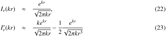as kr → ∞ (see Olver et al. 2010).

Thus, $\begin{array}{ccc}& & \frac{{\mathit{K}}_{\mathit{\nu }}^{\mathrm{\prime }}\mathrm{\left(}\mathit{kr}\mathrm{\right)}}{{\mathit{K}}_{\mathit{\nu }}\mathrm{\left(}\mathit{kr}\mathrm{\right)}}\mathrm{=}\mathit{k}\mathrm{-}\frac{\mathrm{1}}{\mathrm{2}\mathit{r}}\mathit{,} \frac{{\mathit{I}}_{\mathit{\nu }}^{\mathrm{\prime }}\mathrm{\left(}\mathit{kr}\mathrm{\right)}}{{\mathit{I}}_{\mathit{\nu }}\mathrm{\left(}\mathit{kr}\mathrm{\right)}}\mathrm{=}\mathit{k}\mathrm{-}\frac{\mathrm{1}}{\mathrm{2}\mathit{r}}\mathit{,}\\ & & \end{array}$(24)The right-hand side of Eq. (17) can then be rearranged, such that $\begin{array}{ccc}& & \frac{{\mathit{\nu }}_{\mathrm{1}}^{\mathrm{2}}\frac{{\mathit{K}}_{{\mathit{\nu }}_{\mathrm{1}}}\mathrm{\left(}\mathit{k}\mathrm{\right(}{\mathit{r}}_{\mathrm{0}}\mathrm{+}\mathit{a}\mathrm{\left)}\mathrm{\right)}{\mathit{K}}_{{\mathit{\nu }}_{\mathit{m}}}^{\mathrm{\prime }}\mathrm{\left(}\mathit{k}\mathrm{\right(}{\mathit{r}}_{\mathrm{0}}\mathrm{+}\mathit{a}\mathrm{\left)}\mathrm{\right)}}{{\mathit{K}}_{{\mathit{\nu }}_{\mathit{m}}}\mathrm{\left(}\mathit{k}\mathrm{\right(}{\mathit{r}}_{\mathrm{0}}\mathrm{+}\mathit{a}\mathrm{\left)}\mathrm{\right)}{\mathit{K}}_{{\mathit{\nu }}_{\mathrm{1}}}^{\mathrm{\prime }}\mathrm{\left(}\mathit{k}\mathrm{\right(}{\mathit{r}}_{\mathrm{0}}\mathrm{+}\mathit{a}\mathrm{\left)}\mathrm{\right)}}\mathrm{-}{\mathit{\nu }}_{\mathit{m}}^{\mathrm{2}}}{{\mathit{\nu }}_{\mathit{m}}^{\mathrm{2}}\frac{{\mathit{I}}_{{\mathit{\nu }}_{\mathit{m}}}\mathrm{\left(}\mathit{k}\mathrm{\right(}{\mathit{r}}_{\mathrm{0}}\mathrm{+}\mathit{a}\mathrm{\left)}\mathrm{\right)}}{{\mathit{K}}_{{\mathit{\nu }}_{\mathit{m}}}\mathrm{\left(}\mathit{k}\mathrm{\right(}{\mathit{r}}_{\mathrm{0}}\mathrm{+}\mathit{a}\mathrm{\left)}\mathrm{\right)}}\mathrm{-}{\mathit{\nu }}_{\mathrm{1}}^{\mathrm{2}}\frac{{\mathit{I}}_{{\mathit{\nu }}_{\mathit{m}}}^{\mathrm{\prime }}\mathrm{\left(}\mathit{k}\mathrm{\right(}{\mathit{r}}_{\mathrm{0}}\mathrm{+}\mathit{a}\mathrm{\left)}\mathrm{\right)}{\mathit{K}}_{{\mathit{\nu }}_{\mathrm{1}}}\mathrm{\left(}\mathit{k}\mathrm{\right(}{\mathit{r}}_{\mathrm{0}}\mathrm{+}\mathit{a}\mathrm{\left)}\mathrm{\right)}}{{\mathit{K}}_{{\mathit{\nu }}_{\mathrm{1}}}^{\mathrm{\prime }}\mathrm{\left(}\mathit{k}\mathrm{\right(}{\mathit{r}}_{\mathrm{0}}\mathrm{+}\mathit{a}\mathrm{\left)}\mathrm{\right)}{\mathit{K}}_{{\mathit{\nu }}_{\mathit{m}}}\mathrm{\left(}\mathit{k}\mathrm{\right(}{\mathit{r}}_{\mathrm{0}}\mathrm{+}\mathit{a}\mathrm{\left)}\mathrm{\right)}}}\mathit{,}\end{array}$(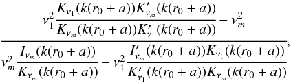25)and from (24) becomes $\begin{array}{ccc}\frac{\mathit{\pi }\mathrm{(}{\mathit{\nu }}_{\mathrm{1}}^{\mathrm{2}}\mathrm{-}{\mathit{\nu }}_{\mathit{m}}^{\mathrm{2}}\mathrm{)}{\mathit{e}}^{\mathrm{-}\mathrm{2}\mathit{kr}}}{{\mathit{\nu }}_{\mathit{m}}^{\mathrm{2}}\mathrm{+}{\mathit{\nu }}_{\mathrm{1}}^{\mathrm{2}}\left(\frac{\mathrm{2}\mathit{kr}\mathrm{-}\mathrm{1}}{\mathrm{2}\mathit{kr}\mathrm{+}\mathrm{1}}\right)}\mathrm{\to }\mathrm{0}\mathit{,}& & \end{array}$(26)as ka → ∞.

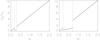Fig. 11 The non-dimensionalised Alfvén speed $\frac{{\mathit{V}}_{\mathrm{A}}}{{\mathit{V}}_{\mathrm{0}}}$ against the wavenumber kr, for the ratios $\frac{{\mathit{V}}_{\mathit{m}}^{\mathrm{2}}}{{\mathit{V}}_{\mathrm{0}}^{\mathrm{2}}}\mathrm{=}\mathrm{0.1}$ and V1 = V0, with kr0 = 0.2, for ka = 0.1.

Thus, the dispersion relation in Eq. (17) reduces to $\begin{array}{ccc}\frac{{\mathit{\nu }}_{\mathrm{0}}^{\mathrm{2}}}{{\mathit{\nu }}_{\mathit{m}}^{\mathrm{2}}}\frac{{\mathit{K}}_{{\mathit{\nu }}_{\mathit{m}}}^{\mathrm{\prime }}\mathrm{\left(}\mathit{k}{\mathit{r}}_{\mathrm{0}}\mathrm{\right)}}{{\mathit{I}}_{{\mathit{\nu }}_{\mathrm{0}}}^{\mathrm{\prime }}\mathrm{\left(}\mathit{k}{\mathit{r}}_{\mathrm{0}}\mathrm{\right)}}\mathrm{=}\frac{{\mathit{K}}_{{\mathit{\nu }}_{\mathit{m}}}\mathrm{\left(}\mathit{k}{\mathit{r}}_{\mathrm{0}}\mathrm{\right)}}{{\mathit{I}}_{{\mathit{\nu }}_{\mathrm{0}}}\mathrm{\left(}\mathit{k}{\mathit{r}}_{\mathrm{0}}\mathrm{\right)}}\mathit{,}& & \end{array}$(27)which is analogous to the two-shell case of Hindman & Jain (2015).

Similar to the current three-shell model, Edwin & Roberts (1983) also studied a cylindrical tube model. However, the Edwin & Roberts (1983) model only considers propagation in a direction parallel to the magnetic field. Here, we have a non-zero axial wavenumber. Additionally, contrary to the Edwin & Roberts (1983) model, here the density is varying with radius. Thus, the two models are not easily comparable (even for V_Ae>V_A>c_e as in Edwin & Roberts 1983). However, it is interesting to note from Fig. 13 the existence of two surface modes in the middle shell as also reported in Fig. 5 of Edwin & Roberts (1983).

6. Conclusions

We have studied the wavemodes of a 3D waveguide of a potential magnetic field arcade. Although the potential field arcade is an idealised situation for the solar corona, it enables us to investigate coronal loop oscillations as fast mode oscillations in the magnetically dominated solar corona. In particular, we investigated in detail the effect of a small region of inhomogeneity in the loop consisting of the two-shell model studied in Hindman & Jain (2015). We also compared the results of the three-shell model with the two-shell model. Similar to the two-shell, our three-shell model also supports the eigenmodes in the radial and azimuthal directions, and depending on the line-of-sight observation, the motion can be a mixture of radial and axial velocities. The elliptical polarisation is quite natural in both models as the radial and axial velocity equations are coupled.

We find that, depending on the thickness of the middle layer, the propagation diagram changes. Not only do a subset of the eigenfrequencies of the two-shell model satisfy the dispersion relation here, but depending on the properties of the middle layer, the reflective property of the wave cavity changes which leads to either suppression of the higher-order radial modes (piecewise linear I model) or the suppression of the evanescent n = 0 mode. In the case of a middle layer which is denser compared with its surroundings (piecewise linear II), the n = 1 radial mode changes its propagating behaviour at large wavenumbers, kr, to evanescence. On the other hand, for a rarer loop embedded inside a denser surrounding, as shown in Fig. 6, the eigenfunctions are similar to the two-shell eigenfunctions (see, e.g. Hindman & Jain 2015).

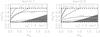Fig. 12 Propagation diagram for the eigenfrequencies $\frac{\mathit{\omega }{\mathit{r}}_{\mathrm{0}}}{{\mathit{V}}_{\mathrm{0}}}$ against the wavenumber kr0, for the ratio $\frac{{\mathit{V}}_{\mathit{m}}^{\mathrm{2}}}{{\mathit{V}}_{\mathrm{0}}^{\mathrm{2}}}\mathrm{=}\mathrm{0.1}$, with kr0 = 0.2, and m = 1, for ka = 0.1 (left) and ka = 0.5 (right).

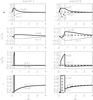Fig. 13 The eigenfunction, φ, radial and axial velocities, normalised ur and uy and polarisation fraction, f, against the wavenumber kr, for the ratio $\frac{{\mathit{V}}_{\mathit{m}}^{\mathrm{2}}}{{\mathit{V}}_{\mathrm{0}}^{\mathrm{2}}}\mathrm{=}\mathrm{0.1}$, with kr0 = 0.2, and m = 1, for ka = 0.1 (left) and ka = 0.5 (right). The curves are normalised with respect to the eigenfunctions, for comparison.

The present study of a three-shell model suggests that the propagating behaviour of the oscillating modes will be quite different in identical coronal loops if the location of observation is different in the respective waveguides. Even for the same eigenfrequency, slightly different inhomogeneity in Alfvén speeds in two different loops could result in very different eigenfunctions for a given wavenumber. One of the important findings of our three-shell model investigation is that some radial modes of the two-shell model (see Hindman & Jain 2015) are absent at the interface, r₀, if there is a small shell of increased density near the interface of the two-shell model. This suggests that some eigenmodes (or eigenfrequencies) may not be observed in such oscillating coronal loops.

We also find that, even in the fundamental mode (n = 0), its propagating behaviour is different depending on the wavenumber if there is a small shell of rarer plasma present within the two-shells considered by Hindman & Jain (2015). The presence and absence of eigenmodes is quite sensitive to the density inhomogeneity in a coronal loop; observation of two similar-looking loops could have very different eigenmodes if the density profiles are slightly different at the observation point. Thus, correct mode identification with multiple wavelength observation at several points on a coronal loop and arcade are essential for understanding the plasma properties of the oscillating loops correctly.

The presence and then subsequent absence of some trapped modes in the two-shell and three-shell models, respectively, suggests that it would be interesting to considering a smoothly varying density for the model arcades. This will introduce a singularity in Eq. (5), which will then introduce damping of modes near the Alfvén resonance. This will be the subject of future work.

Acknowledgments

We acknowledge the SoMaS (University of Sheffield) GTA funding. We thank the anonymous referee for suggesting improvements to the manuscript.

References

All Figures

	Fig. 1 Propagation diagram for the eigenfrequencies $\frac{\mathit{\omega }{\mathit{r}}_{\mathrm{0}}}{{\mathit{V}}_{\mathrm{0}}}$ against the wavenumber kr0, for the ratio$\frac{{\mathit{V}}_{\mathrm{1}}^{\mathrm{2}}}{{\mathit{V}}_{\mathrm{0}}^{\mathrm{2}}}\mathrm{=}\mathrm{0.1}$, and m = 1, for kb = 0.01 (left) and kb = 0.5 (right).
In the text

Fig. 2 The non-dimensionalised Alfvén speed $\frac{{\mathit{V}}_{\mathrm{A}}}{{\mathit{V}}_{\mathrm{0}}}$ against the wavenumber kr, for a) ${\mathit{\nu }}_{\mathit{m}}^{\mathrm{2}}\mathit{>}\mathrm{0}$: $\frac{{\mathit{V}}_{\mathit{m}}^{\mathrm{2}}}{{\mathit{V}}_{\mathrm{0}}^{\mathrm{2}}}\mathrm{=}\mathrm{0.5}$ (top panel), $\frac{{\mathit{V}}_{\mathit{m}}^{\mathrm{2}}}{{\mathit{V}}_{\mathrm{0}}^{\mathrm{2}}}\mathrm{=}\mathrm{2}$ (middle panel), and b) ${\mathit{\nu }}_{\mathit{m}}^{\mathrm{2}}\mathit{<}\mathrm{0}$: $\frac{{\mathit{V}}_{\mathit{m}}^{\mathrm{2}}}{{\mathit{V}}_{\mathrm{0}}^{\mathrm{2}}}\mathrm{=}\mathrm{0.05}$ (bottom panel). In all cases, $\frac{{\mathit{V}}_{\mathrm{1}}^{\mathrm{2}}}{{\mathit{V}}_{\mathrm{0}}^{\mathrm{2}}}\mathrm{=}\mathrm{0.1}$ and kr0 = 0.2, for ka = 0.1 (left) and ka = 0.5 (right).

In the text

Fig. 3 Case I: ${\mathit{\nu }}_{\mathit{m}}^{\mathrm{2}}\mathit{>}\mathrm{0}$. Propagation diagram for the eigenfrequencies $\frac{\mathit{\omega }{\mathit{r}}_{\mathrm{0}}}{{\mathit{V}}_{\mathrm{0}}}$ against the wavenumber kr0, for the ratios $\frac{{\mathit{V}}_{\mathit{m}}^{\mathrm{2}}}{{\mathit{V}}_{\mathrm{0}}^{\mathrm{2}}}\mathrm{=}\mathrm{0.5}$ and $\frac{{\mathit{V}}_{\mathrm{1}}^{\mathrm{2}}}{{\mathit{V}}_{\mathrm{0}}^{\mathrm{2}}}\mathrm{=}\mathrm{0.1}$, and m = 1, for ka = 0.1 (left) and ka = 0.5 (right).

In the text

Fig. 4 Case I: ${\mathit{\nu }}_{\mathit{m}}^{\mathrm{2}}\mathit{>}\mathrm{0}$. The eigenfunction, φ, normalised radial and axial velocities, ur and uy and polarisation fraction, f, against the wavenumber kr, for the ratios $\frac{{\mathit{V}}_{\mathit{m}}^{\mathrm{2}}}{{\mathit{V}}_{\mathrm{0}}^{\mathrm{2}}}\mathrm{=}\mathrm{1}$ and $\frac{{\mathit{V}}_{\mathrm{1}}^{\mathrm{2}}}{{\mathit{V}}_{\mathrm{0}}^{\mathrm{2}}}\mathrm{=}\mathrm{0.1}$, kr0 = 0.2, and m = 1, for ka = 0 (left column). This is analogous to the two-shell case. The middle column and right column are for the cases $\frac{{\mathit{V}}_{\mathit{m}}^{\mathrm{2}}}{{\mathit{V}}_{\mathrm{0}}^{\mathrm{2}}}\mathrm{=}\mathrm{0.5}$ and $\frac{{\mathit{V}}_{\mathrm{1}}^{\mathrm{2}}}{{\mathit{V}}_{\mathrm{0}}^{\mathrm{2}}}\mathrm{=}\mathrm{0.1}$, with kr0 = 0.2, and m = 1, for ka = 0.1 and ka = 0.5, respectively. The curves are normalised with respect to the eigenfunctions, for comparison.

In the text

	Fig. 5 Same as Fig. 3, except for $\frac{{\mathit{V}}_{\mathit{m}}^{\mathrm{2}}}{{\mathit{V}}_{\mathrm{0}}^{\mathrm{2}}}\mathrm{=}\mathrm{2}$.
In the text

	Fig. 6 Same as Fig. 4, except $\frac{{\mathit{V}}_{\mathit{m}}^{\mathrm{2}}}{{\mathit{V}}_{\mathrm{0}}^{\mathrm{2}}}\mathrm{=}\mathrm{2}$.
In the text

	Fig. 7 Case II: ${\mathit{\nu }}_{\mathit{m}}^{\mathrm{2}}\mathit{<}\mathrm{0}$. All parameters the same as in Fig. 4.
In the text

	Fig. 8 Case II: ${\mathit{\nu }}_{\mathit{m}}^{\mathrm{2}}\mathit{<}\mathrm{0}$. All parameters the same as in Fig. 4.
In the text

	Fig. 9 Same as Fig. 7, except $\frac{{\mathit{V}}_{\mathit{m}}^{\mathrm{2}}}{{\mathit{V}}_{\mathrm{0}}^{\mathrm{2}}}\mathrm{=}\mathrm{0.05}$.
In the text

	Fig. 10 Same as Fig. 8, except $\frac{{\mathit{V}}_{\mathit{m}}^{\mathrm{2}}}{{\mathit{V}}_{\mathrm{0}}^{\mathrm{2}}}\mathrm{=}\mathrm{0.05}$.
In the text

	Fig. 11 The non-dimensionalised Alfvén speed $\frac{{\mathit{V}}_{\mathrm{A}}}{{\mathit{V}}_{\mathrm{0}}}$ against the wavenumber kr, for the ratios $\frac{{\mathit{V}}_{\mathit{m}}^{\mathrm{2}}}{{\mathit{V}}_{\mathrm{0}}^{\mathrm{2}}}\mathrm{=}\mathrm{0.1}$ and V1 = V0, with kr0 = 0.2, for ka = 0.1.
In the text

	Fig. 12 Propagation diagram for the eigenfrequencies $\frac{\mathit{\omega }{\mathit{r}}_{\mathrm{0}}}{{\mathit{V}}_{\mathrm{0}}}$ against the wavenumber kr0, for the ratio $\frac{{\mathit{V}}_{\mathit{m}}^{\mathrm{2}}}{{\mathit{V}}_{\mathrm{0}}^{\mathrm{2}}}\mathrm{=}\mathrm{0.1}$, with kr0 = 0.2, and m = 1, for ka = 0.1 (left) and ka = 0.5 (right).
In the text

Fig. 13 The eigenfunction, φ, radial and axial velocities, normalised ur and uy and polarisation fraction, f, against the wavenumber kr, for the ratio $\frac{{\mathit{V}}_{\mathit{m}}^{\mathrm{2}}}{{\mathit{V}}_{\mathrm{0}}^{\mathrm{2}}}\mathrm{=}\mathrm{0.1}$, with kr0 = 0.2, and m = 1, for ka = 0.1 (left) and ka = 0.5 (right). The curves are normalised with respect to the eigenfunctions, for comparison.

In the text

References

- Abramowitz, M., & Stegun, I. A. 1964, Handbook of Mathematical Functions (Dover Publications) [Google Scholar]
- Andries, J., Van Doorsselaere, T., Roberts, B., et al. 2009, Space Sci. Rev., 149, 3 [NASA ADS] [CrossRef] [Google Scholar]
- Appert, K., Gruber, R., & Vaclavik, J. 1974, Physics of Fluids, 17, 1471 [NASA ADS] [CrossRef] [Google Scholar]
- Aschwanden, M. J. 2005, Physics of the Solar Corona: An Introduction with Problems and Solutions (Praxis Publishing) [Google Scholar]
- Aschwanden, M. J., & Schrijver, C. J. 2011, ApJ, 736, 102 [NASA ADS] [CrossRef] [Google Scholar]
- Aschwanden, M. J., Fletcher, L., Schrijver, C. J., & Alexander, D. 1999, ApJ, 520, 880 [NASA ADS] [CrossRef] [Google Scholar]
- Carrion, P. M., Hasegawa, A., Patton, W., & Prakash, M. 1988, Columbia Univ. Annual Report [Google Scholar]
- Dunster, T. M. 1990, SIAM J. Math. Anal., 21, 995 [CrossRef] [Google Scholar]
- Edwin, P. M., & Roberts, B. 1983, Sol. Phys., 88, 179 [NASA ADS] [CrossRef] [Google Scholar]
- Gil, A., Segura, J., & Temme, N. M. 2004, ACM Trans Math Software, 30, 159 [CrossRef] [Google Scholar]
- Goossens, M., Andries, J., & Ashwanden, M. 2002, A&A, 394, L39 [NASA ADS] [CrossRef] [EDP Sciences] [Google Scholar]
- Hindman, B. W., & Jain, R. 2014, ApJ, 784, 103 [NASA ADS] [CrossRef] [Google Scholar]
- Hindman, B. W., & Jain, R. 2015, ApJ, 814, 105 [NASA ADS] [CrossRef] [Google Scholar]
- Jain, R., Maurya, R. A., & Hindman, B. W. 2015, ApJ, 804, L19 [NASA ADS] [CrossRef] [Google Scholar]
- Khongorova, O. V., Mikhalyaev, B. B., & Ruderman, M. S. 2012, Sol. Phys., 280, 153 [NASA ADS] [CrossRef] [Google Scholar]
- Li, H., Liu, Y., & Tam, K. V. 2017, ApJ, 842, 99 [NASA ADS] [CrossRef] [Google Scholar]
- Liu, W., & Ofman, L. 2014, Sol. Phys., 289, 3233 [NASA ADS] [CrossRef] [Google Scholar]
- Melrose, D. B. 1980, Plasma Astrophysics, Vol. 1 (Gordon and Breach, Science Publishers) [Google Scholar]
- Nakariakov, V., & Ofman, L. 2001, A&A, 372, L53 [NASA ADS] [CrossRef] [EDP Sciences] [Google Scholar]
- Nakariakov, V., & Verwichte, E. 2005, Liv. Rev. Sol. Phys., 2, 3 [Google Scholar]
- Nakariakov, V., Ofman, L., DeLuca, E., Roberts, B., & Davila, J. M. 1999, Science, 285, 862 [NASA ADS] [CrossRef] [PubMed] [Google Scholar]
- Ofman, L., Parisi, M., & Srivastava, A. K. 2015, A&A, 582, A75 [NASA ADS] [CrossRef] [EDP Sciences] [Google Scholar]
- Olver, F. W. J., Lozier, D. W., Boisvert, R. F., & Clark, C. W. 2010, NIST Handbook of Mathematics Functions (Cambridge Univ. Press) [Google Scholar]
- Press, W. H., Teukolsky, S. A., Vetterling, W. T., & Flannery, B. P. 2007, Numerical Recipes: The Art of Scientific Computing, 3rd edn. (Cambridge Univ. Press) [Google Scholar]
- Ruderman, M. S., & Roberts, B. 2002, ApJ, 577, 475 [NASA ADS] [CrossRef] [Google Scholar]
- Sakurai, T., Goossens, M., & Hollweg, J. V. 1991, Sol. Phys., 133, 227 [NASA ADS] [CrossRef] [Google Scholar]
- Schrijver, C. J., Aschwanden, M., & Title, A. 2002, Sol. Phys., 206, 69 [NASA ADS] [CrossRef] [Google Scholar]
- Verwichte, E., Nakariakov, V. M., Ofman, L., & DeLuca, E. E. 2004, Sol. Phys., 223, 77 [NASA ADS] [CrossRef] [Google Scholar]
- Verwichte, E., Foullon, C., & Nakariakov, V. 2006, A&A, 449, 769 [NASA ADS] [CrossRef] [EDP Sciences] [Google Scholar]
- Verwichte, E., Aschwanden, M. J., Van Doorrselaere, T., Foullon, C., & Nakariakov, V. M. 2009, ApJ, 698, 397 [NASA ADS] [CrossRef] [Google Scholar]