| Issue |
A&A
Volume 607, November 2017
|
|
|---|---|---|
| Article Number | A50 | |
| Number of page(s) | 15 | |
| Section | Astrophysical processes | |
| DOI | https://doi.org/10.1051/0004-6361/201630169 | |
| Published online | 10 November 2017 | |
Master equation theory applied to the redistribution of polarized radiation in the weak radiation field limit
V. The two-term atom
LESIA, Observatoire de Paris, PSL Research University, CNRS, Sorbonne Universités, UPMC Univ. Paris 06, Univ. Paris Diderot, Sorbonne Paris Cité, 5 place Jules Janssen, 92190 Meudon, France
e-mail: This email address is being protected from spambots. You need JavaScript enabled to view it.
Received: 30 November 2016
Accepted: 24 July 2017
Abstract
Context. In previous papers of this series, we presented a formalism able to account for both statistical equilibrium of a multilevel atom and coherent and incoherent scatterings (partial redistribution).
Aims. This paper provides theoretical expressions of the redistribution function for the two-term atom. This redistribution function includes both coherent (RII) and incoherent (RIII) scattering contributions with their branching ratios.
Methods. The expressions were derived by applying the formalism outlined above. The statistical equilibrium equation for the atomic density matrix is first formally solved in the case of the two-term atom with unpolarized and infinitely sharp lower levels. Then the redistribution function is derived by substituting this solution for the expression of the emissivity.
Results. Expressions are provided for both magnetic and non-magnetic cases. Atomic fine structure is taken into account. Expressions are also separately provided under zero and non-zero hyperfine structure.
Conclusions. Redistribution functions are widely used in radiative transfer codes. In our formulation, collisional transitions between Zeeman sublevels within an atomic level (depolarizing collisions effect) are taken into account when possible (i.e., in the non-magnetic case). However, the need for a formal solution of the statistical equilibrium as a preliminary step prevents us from taking into account collisional transfers between the levels of the upper term. Accounting for these collisional transfers could be done via a numerical solution of the statistical equilibrium equation system.
Key words: atomic processes / line: formation / line: profiles / magnetic fields / polarization / radiative transfer
© ESO, 2017
1. Introduction
The redistribution function in radiative transfer expresses the probability of appearance of an emitted or scattered photon of frequency ν and direction Ω in the presence of an incoming photon of frequency ν1 and direction Ω1. The incoming and the outgoing photons can be polarized. In this work, we follow the convention of describing polarized light through the Stokes vector (S0,S1,S2,S3) ≡ (I,Q,U,V), where I is the radiation intensity, Q and U are two linearly independent states of linear polarization, and V represents circular polarization.
The first expressions of the redistribution function in different cases were heuristically derived by Hummer (1962), without taking into account polarization. He distinguished frequency coherent scattering, denoted as case II with corresponding redistribution function RII which includes a δ(ν−ν1) frequency conservation function, and incoherent scattering, denoted as case III with redistribution function RIII, where the frequencies of the incoming and outgoing photons are independent. Omont et al. (1972) gave a quantum mechanical basis to this formulation, and they were able to provide the branching ratios that weight both coherent and incoherent scattering contributions (see their well-known Eq. (60) for the case of an infinitely sharp lower level). The general case where both frequency coherent and incoherent scattering contribute is known as partial frequency redistribution (PRD). When only incoherent scattering contributes, which is the case of scattering in spectral line cores, it is known as complete frequency redistribution (CRD).
The redistribution function governs the scattering term of the radiative transfer equation (see, e.g., Mihalas 1978). As a consequence, redistribution functions are widely used in the modeling of radiation from stellar atmospheres out of local thermodynamical equilibrium (NLTE). However, the mechanism modeled by the redistribution function is scattering, where a photon is absorbed and then reemitted in a spectral line, possibly coherently in the far wings. The description of the two coupled processes (absorption and emission) requires the solution of the statistical equilibrium of the atomic levels as a preliminary step. For a two-level atom, there is formally only one statistical equilibrium equation expressing the atomic density matrix of the upper level in terms of that of the lower level. Its analytic solution is readily derived (even in the presence of polarization), and the redistribution function follows as a result. In the case of a greater number of levels, the solution becomes much more involved. Attempts were done for the three-level atom. An analytic solution is still possible in this case. This is the equivalent two-level approximation (Hubený et al. 1983). For more than three levels the solution can only be achieved numerically.
The case of the two-term atom with unpolarized and infinitely sharp lower levels is a particular case of multilevel atom. Each level is defined by its quantum numbers (L,S,J) with a given orbital quantum number for each term, Lℓ in the lower term and Lu in the upper term. S is the spin angular momentum quantum number, which for allowed transitions is the same for both terms; and J is the total angular momentum quantum number defined by J = L + S. Due to this vector addition of angular momenta, there can be multiple values of J for both the upper ( ) and lower (
 ) terms. This structure is responsible for D1-D2 pairs of lines with Lℓ = 0,Lu = 1 and S = 1/2, which results in one single lower level Jℓ = 1/2 and two upper levels Ju = 1/2 and
  , as for the Na i D1-D2 lines. Other atoms or ions can be seen in such a structure, and their interest was recently increased by the observations by Stenflo et al. (2000a,b), who recorded some linear polarization in the so-called second solar spectrum of some D1 lines, which are in principle unpolarizable having Ju = 1/2 < 1. The second solar spectrum is the spectrum of the linear polarization formed by scattering and observed close to the solar limb, as defined in Stenflo & Keller (1997).
The interest raised by this problem led several teams to investigate the question by modeling the linear polarization formed by scattering in such lines. However, traditional methods of radiative transfer with partial redistribution based on the works of Hummer (1962) and Omont et al. (1972, Eq. (60)) cannot be readily adapted to the treatment of polarized line formation in these complex two-term transitions, which need to take into account the presence of fine structure as well as the effect of the magnetic field. Empirical attempts at generalizing the redistribution function to the polarized case, also including the effects of fine structure and magnetic fields (Smitha et al. 2011b, 2013a; Belluzzi & Trujillo Bueno 2014) have been proposed. Hyperfine structure was also considered (Smitha et al. 2012b; Sowmya et al. 2014b). These generalizations were exploited in a series of papers for comparison with the observations (Smitha et al. 2011a, 2012a, 2013b, 2014; Belluzzi et al. 2015, 2012; Belluzzi & Trujillo Bueno 2012, 2013; Sowmya et al. 2014a).
However, when compared with the results of a formal theoretical derivation, it appears that these empirical expressions are not fully correct. The aim of the present paper is to publish the correct expressions derived from first principles. The correction concerns essentially the branching ratios that weight the frequency coherent RII and incoherent RIII terms. In fact, we find a contribution of the magnetic field (Zeeman effect) and of the fine (or hyperfine) structure inside these branching ratios, which were missed by Smitha et al. (2013a) and partly missed by Belluzzi & Trujillo Bueno (2014).
Alsina Ballester et al. (2016) recently studied the polarization of the Mg II k line, which is a D2-type line, including the effects of a magnetic field. Because their study was spectrally close to the line, they applied the two-level formalism of Bommier (1997b). del Pino Alemán et al. (2016) studied the polarization of the full Mg II h-k doublet, also taking into account the effects of fine structure and quantum interference in the upper term. They apply the formalism of Casini et al. (2014), who derived a theoretical redistribution function including polarization, fine and hyperfine structure. However, the final result of Casini et al. (2014) can be applied only in the collisionless regime (pure RII). del Pino Alemán et al. (2016) made use of a generalization of the formalism of Casini et al. (2014) to include collisional effects by modifying the branching ratios in a “physically consistent” manner (following their words at the top of the left column, p. 2), but without providing explicit forms of these branching ratios. Providing these ratios is the object of the present paper. Recently, Casini et al. (2017) reinvestigated this question in greater detail. Their final result is given in a compact form by their Eq. (20), which is the same as Eq. (1) of del Pino Alemán et al. (2016). It is comprised of three different added contributions, as is our final result (see Eq. (30) and seq.), which is, however, presented here in its fully explicit algebraic form.
The object of the present paper is to derive branching ratios and associated redistribution functions from the multilevel/multiline general formalism of statistical equilibrium of the atomic density matrix and radiative transfer equations recently published by Bommier (2016a), derived itself from first principles following the method outlined in Bommier (1997a). For the derivation of the redistribution function, a necessary first step is to formally solve the statistical equilibrium problem for the atomic density matrix of the upper state. To this end, the lower state is assumed to be unpolarized and infinitely sharp (Sect. 2); polarization and magnetic fields are considered there. Section 3 provides the redistribution function in the presence of a magnetic field. Section 4 provides instead the redistribution function in the particular case of zero magnetic field. In the concluding Sect. 5, we outline the main limitation of this formalism, which is that collisional transfer between the two fine-structure upper levels cannot be taken into account. In the solar atmosphere, these collisional transfers are due to collisions with neutral hydrogen atoms, which are also responsible for level depolarization due to collisional transitions between the Zeeman sublevels inside a given level. The two rates for the depolarizing collisions in a given level and the collisional transfer between the upper term fine-structure levels are, unfortunately, of the same order of magnitude (see, e.g., Kerkeni & Bommier 2002, Eqs. (11)–(13)). The effects of level depolarizing collision rates can be taken into account in the non-magnetic case (which is why the results of Sect. 4 are not trivially an extension of the magnetic case of Sect. 3). However, collisional transfers cannot be taken into account at all because their presence prevents the derivation of a formal solution of the statistical equilibrium system of equations because several upper levels are coupled by these collisional transfers. A numerical solution of the statistical equilibrium system of equations is required for the solution of the full problem where all required rates are considered. A numerical solution of the statistical equilibrium equations coupled with the radiative transfer equation is under way (Bommier 2016b). This new numerical approach to the solution of the coupled problem does not make use of a redistribution function.
It should be noted that our present derivation is free of any flat spectrum approximation about the incident radiation field.
2. Two-term statistical equilibrium analytical resolution
2.1. Expression of the statistical equilibrium equation
We write the statistical equilibrium equation for an excited-level coherence  where αu represents the set of quantum numbers necessary to specify the atomic term configuration, including LuS. The lower term is assumed to be infinitely sharp, i.e. its lifetime is infinite. In other words, the absorption probability B(αℓLℓ → αuLu)Iν and the inelastic collision excitation probability C(αℓLℓ → αuLu) are very small with respect to the radiative de-excitation probability A(αuLu → αℓLℓ). This assumes that the radiation field in the medium is weak (see the definition in Sect. 2 of Bommier 1997a). Because of the stated condition of the infinite lifetime of the lower term, we can assume that the lower levels are completely unpolarized, since the presence of depolarizing collisions will effectively destroy any atomic polarization in the lower term. Thus, only diagonal elements
  of the lower-term atomic density matrix must be considered. From Eq. (9) of Bommier (2016a) one then has
 ![Mathematical equation: \begin{equation} \begin{array}{l} \medskip \dfrac{\mathrm{d}}{\mathrm{d}t}\ ^{\alpha _{\rm u}J_{\rm u}J_{\rm u}^{\prime }}\rho _{M_{\rm u}M_{\rm u}^{\prime }}\left( \vec{r},\vec{v}\right) =-\dfrac{\mathrm{ i}\Delta E_{M_{\rm u}M_{\rm u}^{\prime }}}{\hbar }\ ^{\alpha _{\rm u}J_{\rm u}J_{\rm u}^{\prime }}\rho _{M_{\rm u}M_{\rm u}^{\prime }}\left( \vec{r},\vec{v}\right) \\ \qquad +\dsum\limits_{J_{\ell }M_{\ell }}^{{}}\ ^{\alpha _{\ell }J_{\ell }J_{\ell }}\rho _{M_{\ell }M_{\ell }}\left( \vec{r},\vec{v}\right) 3B(\alpha _{\ell }L_{\ell }\rightarrow \alpha _{\rm u}L_{\rm u})(2L_{\ell }+1)(2J_{\ell }+1) \sqrt{(2J_{\rm u}+1)(2J_{\rm u}^{\prime }+1)} \\ \qquad \times \left\{ \begin{array}{ccc} J_{\rm u} & 1 & J_{\ell } \\ L_{\ell } & S & L_{\rm u} \end{array} \right\} \left\{ \begin{array}{ccc} J_{\rm u}^{\prime } & 1 & J_{\ell } \\ L_{\ell } & S & L_{\rm u} \end{array} \right\} \left( \begin{array}{ccc} J_{\rm u} & 1 & J_{\ell } \\ -M_{\rm u} & p & M_{\ell } \end{array} \right) \left( \begin{array}{ccc} J_{\rm u}^{\prime } & 1 & J_{\ell } \\ -M_{\rm u}^{\prime } & p^{\prime } & M_{\ell } \end{array} \right) \\ \qquad \times (-1)^{J_{\rm u}-J_{\rm u}^{\prime }}\dint \mathrm{d}\nu _{1}\doint \dfrac{\mathrm{d}\vec{\Omega}_{1}}{4\pi }\mathcal{I}_{-p-p^{\prime }}(\nu _{1},\vec{\Omega}_{1})\left[ \dfrac{1}{2}\Phi _{ba}\left( \nu _{M_{\rm u}^{\prime }M_{\ell }}-\tilde{\nu}_{1}\right) +\dfrac{1}{2}\Phi _{ba}^{\ast }\left( \nu _{M_{\rm u}M_{\ell }}-\tilde{\nu}_{1}\right) \right] \\ \qquad -\dfrac{1}{2}\dsum\limits_{J_{\rm u}^{\prime \prime }}\left\{ \dsum\limits_{J_{\ell }M_{\ell }}\ ^{\alpha _{\rm u}J_{\rm u}^{\prime \prime }J_{\rm u}^{\prime }}\rho _{M_{\rm u}M_{\rm u}^{\prime }}\left( \vec{r},\vec{v}\right) A(\alpha _{\rm u}L_{\rm u}\rightarrow \alpha _{\ell }L_{\ell })(2L_{\rm u}+1)(2J_{\ell }+1)\sqrt{(2J_{\rm u}+1)(2J_{\rm u}^{\prime \prime }+1)}\right. \\ \qquad \times (-1)^{J_{\rm u}^{\prime \prime }-J_{\rm u}}\left\{ \begin{array}{ccc} J_{\rm u} & 1 & J_{\ell } \\ L_{\ell } & S & L_{\rm u} \end{array} \right\} \left\{ \begin{array}{ccc} J_{\rm u}^{\prime \prime } & 1 & J_{\ell } \\ L_{\ell } & S & L_{\rm u} \end{array} \right\} \left( \begin{array}{ccc} J_{\ell } & 1 & J_{\rm u} \\ -M_{\ell } & -p & M_{\rm u} \end{array} \right) \left( \begin{array}{ccc} J_{\ell } & 1 & J_{\rm u}^{\prime \prime } \\ -M_{\ell } & -p & M_{\rm u} \end{array} \right) \\ \qquad +\dsum\limits_{J_{\ell }M_{\ell }}\ ^{\alpha _{\rm u}J_{\rm u}J_{\rm u}^{\prime \prime }}\rho _{M_{\rm u}M_{\rm u}^{\prime }}\left( \vec{r},\vec{v}\right) A(\alpha _{\rm u}L_{\rm u}\rightarrow \alpha _{\ell }L_{\ell })(2L_{\rm u}+1)(2J_{\ell }+1)\sqrt{ (2J_{\rm u}+1)(2J_{\rm u}^{\prime \prime }+1)} \\ \qquad \times \left. (-1)^{J_{\rm u}^{\prime \prime }-J_{\rm u}^{\prime }}\left\{ \begin{array}{ccc} J_{\rm u}^{\prime } & 1 & J_{\ell } \\ L_{\ell } & S & L_{\rm u} \end{array} \right\} \left\{ \begin{array}{ccc} J_{\rm u}^{\prime \prime } & 1 & J_{\ell } \\ L_{\ell } & S & L_{\rm u} \end{array} \right\} \left( \begin{array}{ccc} J_{\ell } & 1 & J_{\rm u}^{\prime } \\ -M_{\ell } & -p^{\prime } & M_{\rm u}^{\prime } \end{array} \right) \left( \begin{array}{ccc} J_{\ell } & 1 & J_{\rm u}^{\prime \prime } \\ -M_{\ell } & -p^{\prime } & M_{\rm u}^{\prime } \end{array} \right) \phantom{\dsum\limits_{x}} \!\!\!\!\!\!\right\} \cdot \end{array} \label{eq -- stateq1} \end{equation}](/articles/aa/full_html/2017/11/aa30169-16/aa30169-16-eq36.png) (1)The first line of this equation accounts for the oscillation effect due to the possible presence of a magnetic field (the Hanle effect). Lines 2–4 describe the creation of the upper level atomic coherence under the effect of radiation absorption from the lower term, and lines 5–8 describe the coherence relaxation under the effect of spontaneous emission. Collisions are neglected for the moment. The atomic density matrix element depends on the atom position r and velocity v.
(1)The first line of this equation accounts for the oscillation effect due to the possible presence of a magnetic field (the Hanle effect). Lines 2–4 describe the creation of the upper level atomic coherence under the effect of radiation absorption from the lower term, and lines 5–8 describe the coherence relaxation under the effect of spontaneous emission. Collisions are neglected for the moment. The atomic density matrix element depends on the atom position r and velocity v.
We denote  the energy difference between the two levels αuJuMu and
 (2)where
  (3)where E(αuJu;B = 0) is the fine structure level energy in the absence of a magnetic field, νL is the Larmor frequency
 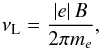 (4)where |e| is the electron charge absolute value, me is the electron mass, B is the magnetic field strength, and gJu is the Landé factor of the upper level αuJu. In Eq. (3) above, the incomplete Paschen-Back effect is ignored; it is addressed below in Sect. 3.3. This effect has to be taken into account when the Zeeman splitting and the fine or hyperfine splitting are of the same order of magnitude.
Similarly, νMuMℓ denotes the frequency of the transition between the two levels αuJuMu and αℓJℓMℓ, and  that of the transition between the two levels and αℓJℓMℓ
![Mathematical equation: \begin{equation} \left\{ \begin{array}{c} \medskip \nu _{M_{\rm u}M_{\ell }}=\left[ E(\alpha _{\rm u}J_{\rm u}M_{\rm u})-E(\alpha _{\ell }J_{\ell }M_{\ell })\right] /h \\ \nu _{M_{\rm u}^{\prime }M_{\ell }}=\left[ E(\alpha _{\rm u}J_{\rm u}^{\prime }M_{\rm u}^{\prime })-E(\alpha _{\ell }J_{\ell }M_{\ell })\right] /h, \end{array} \ \right. \end{equation}](/articles/aa/full_html/2017/11/aa30169-16/aa30169-16-eq56.png) (5)where h is the Planck constant. The expression
(5)where h is the Planck constant. The expression  denotes the tensor of the incident radiation of frequency ν1 and direction Ω1. This tensor is defined in Sect. 5.11 of the monograph by Landi Degl’Innocenti & Landolfi (2004), devoted to the spherical tensors for polarimetry. It is related to the Stokes parameters of the incident radiation by
 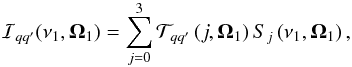 (6)where Sj (j = 0,1,2,3) is one of the Stokes parameters, and Tqq′(j,Ω1) is the spherical tensor for polarimetry defined and tabulated by Landi Degl’Innocenti & Landolfi (2004, Table 5.3, p. 206). Given the direction Ω1 of the incident radiation, the Doppler effect has to be accounted for in the absorption profiles by the atom with velocity v
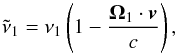 (7)see also Sect. 3.1 of Bommier (2016a) about Doppler (or velocity) redistribution. The parameter Φba denotes the Lorentz absorption profile, which has the same width 2γba (full width at half maximum) for all the components of the same multiplet. The definition of the width of the profile, which includes the effects of collisions, can be found in Sect. 3.4 of Bommier (2016a).
Accounting for  (8)and analogously for
  , and
, and  (9)lines 5–8 of the above Eq. (1), which account for the coherence destruction processes, simply reduce into
  (10)which is also
 ![Mathematical equation: \begin{equation} -\sum_{J_{\ell }}\frac{1}{2}\left[ A(\alpha _{\rm u}L_{\rm u}J_{\rm u}\rightarrow \alpha _{\ell }L_{\ell }J_{\ell })+A(\alpha _{\rm u}L_{\rm u}J_{\rm u}^{\prime }\rightarrow \alpha _{\ell }L_{\ell }J_{\ell })\right] \ ^{\alpha _{\rm u}J_{\rm u}J_{\rm u}^{\prime }}\rho _{M_{\rm u}M_{\rm u}^{\prime }}\left( \vec{r},\vec{v}\right) , \label{eq -- As for Js} \end{equation}](/articles/aa/full_html/2017/11/aa30169-16/aa30169-16-eq70.png) (11)from
(11)from  (12)and similarly for
  .
.
The lower level is assumed to be infinitely sharp and unpolarized. Accordingly, the Zeeman sublevels are equally populated as  (13)This also assumes that the lower term remains much more populated than the upper term. Indeed, the ratio of the upper term population to the lower term population is at most on the order of the number of photons per mode
  , and in stellar atmosphere physics this number is usually such that
  , which is the weak radiation field condition (Bommier 1997a, Sect. 2). As a consequence, the population ratio is ≪1. By simply neglecting the upper term population with respect to the lower term one, both the above condition and the normalization condition of the atomic density matrix Trρ = 1 are satisfied. Outside the weak radiation field condition, the whole present formalism cannot be applied, as discussed in Bommier (1997a). Moreover, the effect of the approximation is even weaker when one finally considers the ratios of the Stokes parameters Q/I,U/I,V/I instead of the Stokes parameters themselves. The important point is that all the lower sublevel populations are equal, and that there are no off-diagonal elements (coherences) in the lower level density matrix. Coherences or unequal sublevel populations in the lower level would invalidate the results of the present paper because they would prevent the analytical solution of the statistical equilibrium as is done in the following section. When these elements are non-negligible with respect to the lower level total population, the statistical equilibrium equations form a system that has to be numerically solved. Apart from this case, a global scaling factor could be applied to these lower sublevel populations without changing the results of the present paper, to which the scaling factor would also have to be applied.
Another consequence of the large lower term population is that the velocity distribution in this term remains Maxwellian. Lines 2–4 of the above Eq. ( 1), which account for the coherence creation processes, can then be rewritten as ![Mathematical equation: \begin{equation} \begin{array}{l} \medskip \dsum\limits_{J_{\ell }M_{\ell }}^{{}}\ 3B(\alpha _{\ell }L_{\ell }\rightarrow \alpha _{\rm u}L_{\rm u})\dfrac{2J_{\ell }+1}{2S+1}\sqrt{ (2J_{\rm u}+1)(2J_{\rm u}^{\prime }+1)}\ (-1)^{J_{\rm u}-J_{\rm u}^{\prime }} \\ \qquad \times \left\{ \begin{array}{ccc} J_{\rm u} & 1 & J_{\ell } \\ L_{\ell } & S & L_{\rm u} \end{array} \right\} \left\{ \begin{array}{ccc} J_{\rm u}^{\prime } & 1 & J_{\ell } \\ L_{\ell } & S & L_{\rm u} \end{array} \right\} \left( \begin{array}{ccc} J_{\rm u} & 1 & J_{\ell } \\ -M_{\rm u} & p & M_{\ell } \end{array} \right) \left( \begin{array}{ccc} J_{\rm u}^{\prime } & 1 & J_{\ell } \\ -M_{\rm u}^{\prime } & p^{\prime } & M_{\ell } \end{array} \right) \\ \qquad \times \dint \mathrm{d}\nu _{1}\doint \dfrac{\mathrm{d}\vec{\Omega} _{1}}{4\pi }\dsum\limits_{j=0}^{3}\mathcal{T}_{-p-p^{\prime }}\left( j,\vec{ \Omega}_{1}\right) S_{j}\left( \nu _{1},\vec{\Omega}_{1}\right) \left[ \dfrac{1}{2}\Phi _{ba}\left( \nu _{M_{\rm u}^{\prime }M_{\ell }}-\tilde{\nu} _{1}\right) +\dfrac{1}{2}\Phi _{ba}^{\ast }\left( \nu _{M_{\rm u}M_{\ell }}- \tilde{\nu}_{1}\right) \right]. \end{array} \end{equation}](/articles/aa/full_html/2017/11/aa30169-16/aa30169-16-eq79.png) (14)
(14)
2.2. Solution of the statistical equilibrium equation
2.2.1. In the presence of a magnetic field
Introducing the spherical tensors for polarimetry (Landi Degl’Innocenti & Landolfi 2004, see Eq. (5.156))  (15)the statistical equilibrium Eq. (1) can be resolved into
 ![Mathematical equation: \begin{equation} \begin{array}{l} \medskip \ ^{\alpha _{\rm u}J_{\rm u}J_{\rm u}^{\prime }}\rho _{M_{\rm u}M_{\rm u}^{\prime }}\left( \vec{r},\vec{v}\right) =\qquad \dfrac{1}{A(\alpha _{\rm u}L_{\rm u}\rightarrow \alpha _{\ell }L_{\ell })+\dfrac{\mathrm{i}\Delta E_{M_{\rm u}M_{\rm u}^{\prime }}}{\hbar }} \\ \qquad \times \dsum\limits_{J_{\ell }M_{\ell }}^{{}}\dsum\limits_{K^{\prime }Q}B(\alpha _{\ell }L_{\ell }\rightarrow \alpha _{\rm u}L_{\rm u})\dfrac{2J_{\ell }+1}{2S+1}\sqrt{(2J_{\rm u}+1)(2J_{\rm u}^{\prime }+1)}\sqrt{3(2K^{\prime }+1)}\ (-1)^{J_{\rm u}-J_{\rm u}^{\prime }+1-p} \\ \qquad \times \left\{ \begin{array}{ccc} J_{\rm u} & 1 & J_{\ell } \\ L_{\ell } & S & L_{\rm u} \end{array} \right\} \left\{ \begin{array}{ccc} J_{\rm u}^{\prime } & 1 & J_{\ell } \\ L_{\ell } & S & L_{\rm u} \end{array} \right\} \left( \begin{array}{ccc} J_{\rm u} & 1 & J_{\ell } \\ -M_{\rm u} & p & M_{\ell } \end{array} \right) \left( \begin{array}{ccc} J_{\rm u}^{\prime } & 1 & J_{\ell } \\ -M_{\rm u}^{\prime } & p^{\prime } & M_{\ell } \end{array} \right) \left( \begin{array}{ccc} 1 & 1 & K^{\prime } \\ -p & p^{\prime } & Q \end{array} \right) \\ \qquad \times \dint \mathrm{d}\nu _{1}\doint \dfrac{\mathrm{d}\vec{\Omega} _{1}}{4\pi }\dsum\limits_{j=0}^{3}\mathcal{T}_{-Q}^{K^{\prime }}(j,\vec{ \Omega}_{1})S_{j}\left( \nu _{1},\vec{\Omega}_{1}\right) \left[ \dfrac{1}{2} \Phi _{ba}\left( \nu _{M_{\rm u}^{\prime }M_{\ell }}-\tilde{\nu}_{1}\right) + \dfrac{1}{2}\Phi _{ba}^{\ast }\left( \nu _{M_{\rm u}M_{\ell }}-\tilde{\nu} _{1}\right) \right]. \end{array} \label{eq-solMM1} \end{equation}](/articles/aa/full_html/2017/11/aa30169-16/aa30169-16-eq81.png) (16)Introducing the spherical components of the density matrix
(16)Introducing the spherical components of the density matrix  with
with  and Q = −K,−K + 1,..., K−1,K as defined by (Landi Degl’Innocenti & Landolfi 2004, see Eq. (3.97))
  (17)the spherical component can be written as
 ![Mathematical equation: \begin{equation} \begin{array}{l} \medskip \ ^{\alpha _{\rm u}J_{\rm u}J_{\rm u}^{\prime }}\rho _{Q}^{K}\left( \vec{r}, \vec{v}\right) =\dsum\limits_{M_{\rm u}M_{\rm u}^{\prime }}\medskip \dfrac{1}{ A(\alpha _{\rm u}L_{\rm u}\rightarrow \alpha _{\ell }L_{\ell })+\dfrac{\mathrm{i} \Delta E_{M_{\rm u}M_{\rm u}^{\prime }}}{\hbar }} \\ \qquad \times \dsum\limits_{J_{\ell }M_{\ell }}^{{}}\dsum\limits_{K^{\prime }}B(\alpha _{\ell }L_{\ell }\rightarrow \alpha _{\rm u}L_{\rm u})\dfrac{2J_{\ell }+1}{2S+1}\sqrt{(2J_{\rm u}+1)(2J_{\rm u}^{\prime }+1)}\sqrt{3(2K+1)(2K^{\prime }+1)}\ (-1)^{J_{\rm u}^{\prime }-M_{\rm u}^{\prime }+1-p^{\prime }} \\ \qquad \times \left\{ \begin{array}{ccc} J_{\rm u} & 1 & J_{\ell } \\ L_{\ell } & S & L_{\rm u} \end{array} \right\} \left\{ \begin{array}{ccc} J_{\rm u}^{\prime } & 1 & J_{\ell } \\ L_{\ell } & S & L_{\rm u} \end{array} \right\} \\ \qquad \times \left( \begin{array}{ccc} J_{\rm u} & 1 & J_{\ell } \\ -M_{\rm u} & p & M_{\ell } \end{array} \right) \left( \begin{array}{ccc} J_{\rm u}^{\prime } & 1 & J_{\ell } \\ -M_{\rm u}^{\prime } & p^{\prime } & M_{\ell } \end{array} \right) \left( \begin{array}{ccc} 1 & 1 & K^{\prime } \\ -p & p^{\prime } & Q \end{array} \right) \left( \begin{array}{ccc} J_{\rm u} & K & J_{\rm u}^{\prime } \\ -M_{\rm u} & Q & M_{\rm u}^{\prime } \end{array} \right) \\ \qquad \times \dint \mathrm{d}\nu _{1}\doint \dfrac{\mathrm{d}\vec{\Omega} _{1}}{4\pi }\dsum\limits_{j=0}^{3}\mathcal{T}_{-Q}^{K^{\prime }}(j,\vec{ \Omega}_{1})S_{j}\left( \nu _{1},\vec{\Omega}_{1}\right) \left[ \dfrac{1}{2} \Phi _{ba}\left( \nu _{M_{\rm u}^{\prime }M_{\ell }}-\tilde{\nu}_{1}\right) + \dfrac{1}{2}\Phi _{ba}^{\ast }\left( \nu _{M_{\rm u}M_{\ell }}-\tilde{\nu} _{1}\right) \right]. \end{array} \label{eq -- solKQ} \end{equation}](/articles/aa/full_html/2017/11/aa30169-16/aa30169-16-eq87.png) (18)In the case of the two-level atom, i.e., when there is one single Ju and one single Jℓ, this equation can be reduced in terms of generalized profiles as defined in Landi Degl’Innocenti et al. (1991). Equation (37) of this paper is thus obtained, which is also Eq. (7) of Bommier (1997b). This is made possible owing to the following relation, which is valid only if
(18)In the case of the two-level atom, i.e., when there is one single Ju and one single Jℓ, this equation can be reduced in terms of generalized profiles as defined in Landi Degl’Innocenti et al. (1991). Equation (37) of this paper is thus obtained, which is also Eq. (7) of Bommier (1997b). This is made possible owing to the following relation, which is valid only if 
 (19)The factorization in Q of permits restricting the summation over Mu and
  to just the second addendum of Eq. (18), leading to the generalized profile and also making possible the introduction of the depolarizing collision factors D(K), as obtained in Bommier (1997b). In the general case of fine structure, when there are several αuJu levels, it is not possible to factorize in terms of Q when
  because the form of is more involved. However, when the magnetic field is zero, does not depend on the magnetic quantum numbers Mu and it simply coincides with
  , which again makes it possible to introduce the depolarizing collision factors D(K), as is done in the following section. However, the depolarizing effect of collisions is thus only partly taken into account (see Sect. 5), and this can be done only in the absence of a magnetic field. The outcome is the numerical solution of the statistical equilibrium equations.
2.2.2. In zero magnetic field
In the absence of a magnetic field, the M indexes in ΔE and ν can be replaced by the J indexes and the sums over the M indexes can be performed. Then, Eq. (16) reduces to ![Mathematical equation: \begin{equation} \begin{array}{l} \medskip \ ^{\alpha _{\rm u}J_{\rm u}J_{\rm u}^{\prime }}\rho _{M_{\rm u}M_{\rm u}^{\prime }}\left( \vec{r},\vec{v}\right) =\medskip \dfrac{1}{A(\alpha _{\rm u}L_{\rm u}\rightarrow \alpha _{\ell }L_{\ell })+\dfrac{\mathrm{i}\Delta E_{J_{\rm u}J_{\rm u}^{\prime }}}{\hbar }} \\ \qquad \times \dsum\limits_{J_{\ell }}^{{}}\dsum\limits_{KQ}B(\alpha _{\ell }L_{\ell }\rightarrow \alpha _{\rm u}L_{\rm u})\dfrac{2J_{\ell }+1}{2S+1} \sqrt{(2J_{\rm u}+1)(2J_{\rm u}^{\prime }+1)}\sqrt{3(2K^{\prime }+1)}\ (-1)^{1+J_{\ell }+2J_{\rm u}-M_{\rm u}^{\prime }} \\ \qquad \times \left\{ \begin{array}{ccc} J_{\rm u} & 1 & J_{\ell } \\ L_{\ell } & S & L_{\rm u} \end{array} \right\} \left\{ \begin{array}{ccc} J_{\rm u}^{\prime } & 1 & J_{\ell } \\ L_{\ell } & S & L_{\rm u} \end{array} \right\} \left\{ \begin{array}{ccc} K^{\prime } & J_{\rm u} & J_{\rm u}^{\prime } \\ J_{\ell } & 1 & 1 \end{array} \right\} \left( \begin{array}{ccc} J_{\rm u} & K^{\prime } & J_{\rm u}^{\prime } \\ -M_{\rm u} & Q & M_{\rm u}^{\prime } \end{array} \right) \\ \qquad \times \dint \mathrm{d}\nu _{1}\doint \dfrac{\mathrm{d}\vec{\Omega} _{1}}{4\pi }\dsum\limits_{j=0}^{3}\mathcal{T}_{-Q}^{K^{\prime }}(j,\vec{ \Omega}_{1})S_{j}\left( \nu _{1},\vec{\Omega}_{1}\right) \left[ \dfrac{1}{2} \Phi _{ba}\left( \nu _{J_{\rm u}^{\prime }J_{\ell }}-\tilde{\nu}_{1}\right) + \dfrac{1}{2}\Phi _{ba}^{\ast }\left( \nu _{J_{\rm u}J_{\ell }}-\tilde{\nu} _{1}\right) \right], \end{array} \end{equation}](/articles/aa/full_html/2017/11/aa30169-16/aa30169-16-eq99.png) (20)where only the sum over Mℓ has been performed, whereas Eq. (18) becomes
(20)where only the sum over Mℓ has been performed, whereas Eq. (18) becomes ![Mathematical equation: \begin{equation} \begin{array}{l} \medskip \ ^{\alpha _{\rm u}J_{\rm u}J_{\rm u}^{\prime }}\rho _{Q}^{K}\left( \vec{r}, \vec{v}\right) =\medskip \dfrac{1}{A(\alpha _{\rm u}L_{\rm u}\rightarrow \alpha _{\ell }L_{\ell })+\dfrac{1}{2}\left[ D^{(K)}(\alpha _{\rm u}J_{\rm u})+D^{(K)}(\alpha _{\rm u}J_{\rm u}^{\prime })\right] +\dfrac{\mathrm{i} \Delta E_{J_{\rm u}J_{\rm u}^{\prime }}}{\hbar }} \\ \qquad \times B(\alpha _{\ell }L_{\ell }\rightarrow \alpha _{\rm u}L_{\rm u}) \dfrac{2J_{\ell }+1}{2S+1}\sqrt{3(2J_{\rm u}+1)(2J_{\rm u}^{\prime }+1)}\ (-1)^{1+J_{\ell }+J_{\rm u}+Q} \\ \qquad \times \left\{ \begin{array}{ccc} J_{\rm u} & 1 & J_{\ell } \\ L_{\ell } & S & L_{\rm u} \end{array} \right\} \left\{ \begin{array}{ccc} J_{\rm u}^{\prime } & 1 & J_{\ell } \\ L_{\ell } & S & L_{\rm u} \end{array} \right\} \left\{ \begin{array}{ccc} K & J_{\rm u} & J_{\rm u}^{\prime } \\ J_{\ell } & 1 & 1 \end{array} \right\} \\ \qquad \times \dint \mathrm{d}\nu _{1}\doint \dfrac{\mathrm{d}\vec{\Omega} _{1}}{4\pi }\dsum\limits_{j=0}^{3}\mathcal{T}_{-Q}^{K}(j,\vec{\Omega} _{1})S_{j}\left( \nu _{1},\vec{\Omega}_{1}\right) \left[ \dfrac{1}{2}\Phi _{ba}\left( \nu _{J_{\rm u}^{\prime }J_{\ell }}-\tilde{\nu}_{1}\right) +\dfrac{1 }{2}\Phi _{ba}^{\ast }\left( \nu _{J_{\rm u}J_{\ell }}-\tilde{\nu}_{1}\right) \right], \end{array} \end{equation}](/articles/aa/full_html/2017/11/aa30169-16/aa30169-16-eq101.png) (21)where the sums over
(21)where the sums over  have been performed, and where one has applied
  (22)The depolarizing collisions have been taken into account here, by adding their contribution in the K-order coherence inverse lifetime contribution and similarly to Eq. (11). This is possible only for the tensorial component
  but not for the dyadic component , as explained below. In addition, this does not account for all the elastic or quasi-elastic collision effects. In the solar atmosphere, these effects are due to collisions with neutral hydrogen atoms. These collisions induce both transitions between Zeeman sublevels and between fine or hyperfine structure levels. Here we only account for the transitions between the Zeeman sublevels and we ignore the other transitions. However, as detailed in Sect. 5, both contributions are of the same order of magnitude. Thus, by so doing we include only a part of the effect of the elastic or quasi-elastic collisions.
An attempt to account for the depolarizing collisions was heuristically proposed by Smitha et al. (2013a), but introducing the same D(K) rate for both αuJu and  states (with D(0) = 0). The above expression is the result of a formal derivation and accounts for the fine structure as far as possible, i.e., in the absence of a magnetic field and in tensorial components. This is the only case where the effect of the transitions between the Zeeman sublevels can be simply accounted for through the D(K)(αuJu) rates. In the general case, this is not possible due to the presence of because the explicit dependence on Mu and
  excessively complicates the formalism. In addition, the transitions between the fine structure levels cannot be accounted for in any case. This was pointed out by Belluzzi & Trujillo Bueno (2014) in their Sect. 3.1, and was the reason why they discarded the whole depolarizing effect of collisions from their formalism. As pointed out by these authors, taking into account all the effects of the collisions with neutral hydrogen requires the numerical solution of the statistical equilibrium.
In the general case of fine structure, as stated in the above, it is not possible to factorize in terms of Q when and in non-zero magnetic fields. The statistical equilibrium equations are then simple only in the dyadic basis. In this basis, the introduction of the depolarizing collisions effect, even limited to those responsible for the D(K) coefficients, leads to the coupling of all the upper level Zeeman sublevel coherences, as visible in the unnumbered equation before Eq. (7.99) of Landi Degl’Innocenti & Landolfi (2004). This coupling prevents an analytical solution of the statistical equilibrium in the dyadic basis from being attained. Transforming into the irreducible tensors basis leads to other couplings, also preventing an analytical solution, due to the non-factorization of  in terms of Q in the presence of a fine structure. This is why it is possible to simply introduce D(K) coefficients only in the zero magnetic field case, when there is a fine structure. The outcome of this problem is the numerical solution of the statistical equilibrium equations.
3. Redistribution function in the presence of a magnetic field
The expression of the redistribution function follows by porting the solution of the statistical equilibrium in the emissivity, which is given in Eqs. (15), (16) of Bommier (2016a). The emissivity represents the emitted light quantity per unit volume and is given by  (23)where the redistribution function Rij(ν,ν1,Ω,Ω1;B) is the joint probability of observing a photon of frequency ν and polarization i emitted in the Ω direction, given a photon of frequency ν1 and polarization j incident along the Ω1 direction, in the presence of a magnetic field B. The parameter kL is the line absorption coefficient
  (24)where
  is the emitter atom or ion density and B(αℓLℓ → αuLu) is the Einstein coefficient for absorption in the line. We recall that the atom lower term is here assumed to be overpopulated, i.e., the entire atomic population is assumed to be in the ground state as defined in Eq. (13); is then also the lower term atom or ion density.
The emission can possibly end in level  of the lower term, which may be different from the initial (αℓLℓSJℓMℓ) level.
The contribution of inelastic collisions has to be considered. For de-excitation, this adds a collisional contribution C(αuLu → αℓLℓ) to the radiative de-excitation probability A(αuLu → αℓLℓ). For excitation, it adds a contribution term besides the radiative excitation term in Eq. (1). This collisional excitation term is at the origin of the well-known Planck source term of the radiative transfer equation, which we will not rewrite here (see for instance Eq. (25) of Belluzzi & Trujillo Bueno 2014).
To simplify notations, we introduce the usual Γ probabilities in the excited term 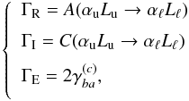 (25)where ΓR is the radiative deexcitation coefficient, ΓI is the inelastic collisional deexcitation coefficient, and ΓE is the elastic collision contribution to line broadening as described in Sahal-Bréchot & Bommier (2014, 2017). The expression of
  in terms of the collisional S and T = 1−S matrices is also given in Eqs. (28), (29) of Bommier (2016a).
The redistribution function as defined in Eq. (23) is normalized to  (26)and not to unity. This is the same for the two-level atom redistribution function defined in Bommier (1997b). This is also the same in Omont et al. (1972); the normalization condition is given in their Eq. (64), which is the same normalization condition as above, and γ is the angle with the reference axis for the linear polarization definition (the direction of positive polarization) in the plane perpendicular to the line of sight (see Fig. 2 in Landi Degl’Innocenti 1983). The redistribution function is not normalized to unity because here it accounts for the total emitted radiation. However, the photon emission generally results from two contributions, scattering of the incident photon on the one hand, and collisional excitation followed by radiative de-excitation on the other. This explains why the result of the scattering contribution is not normalized to unity. However, other authors prefer to normalize their redistribution function to unity (see, e.g., Mihalas 1978, Eqs. (2)–(7)). In this case, the effect of the competing collisional excitation is accounted for by the (1−ϵ) coefficient, which factorizes the scattering contribution in the transfer equation (see Eqs. (2)–(36), (2)–(41) and (13)–(92)). Here,
  . In order to apply the formulae we present in the following, it is convenient to multiply our redistribution functions by
  . Belluzzi & Trujillo Bueno (2014) apply the same normalization as ours to their redistribution functions (see their Eqs. (1), (7)–(12) and following unnumbered equations). As the results of Casini et al. (2014) can only be applied in the collisionless regime, the two possible normalizations described above are identical and are both equal to unity in this regime.
The redistribution function normalization condition is based on the following normalization property of the irreducible spherical tensors for polarimetry (Landi Degl’Innocenti 1984)  (27)as can be derived for instance from Table 1 in Bommier (1997b).
Considering both the second-order  and fourth-order
  contributions to the emissivity as defined in Eqs. (15), (16) of Bommier (2016a), the following expressions can be derived, which contain both frequency coherent RII and frequency incoherent RIII and their branching ratios.
3.1. Considering only fine structure
Let us first provide a few formulae useful for the calculation. In the fourth-order emissivity, there is a profile  . In the case of the two-term atom, c = a and the profile width is the lower term width γa, which tends towards zero because we have assumed that the lower level is infinitely sharp γa− → 0. Therefore,
  (28)where
  stands for the Cauchy principal value.
Equation (3) in Bommier (1997b), which transforms a profile product into a profile sum, is also useful for the calculation. In the present notation, this is ![Mathematical equation: \begin{equation} \dfrac{1}{2}\Phi _{ba}\left( \nu _{M_{\rm u}^{\prime }M_{\ell }}-\tilde{\nu} _{1}\right) \ \dfrac{1}{2}\Phi _{ba}^{\ast }\left( \nu _{M_{\rm u}M_{\ell }}- \tilde{\nu}_{1}\right) =\frac{1}{2\gamma _{ba}+\dfrac{\mathrm{i}\Delta E_{M_{\rm u}M_{\rm u}^{\prime }}}{\hbar }}\left[ \dfrac{1}{2}\Phi _{ba}\left( \nu _{M_{\rm u}^{\prime }M_{\ell }}-\tilde{\nu}_{1}\right) +\dfrac{1}{2}\Phi _{ba}^{\ast }\left( \nu _{M_{\rm u}M_{\ell }}-\tilde{\nu}_{1}\right) \right] , \end{equation}](/articles/aa/full_html/2017/11/aa30169-16/aa30169-16-eq144.png) (29)where 2γba is the full line width at half maximum (see Sect. 3.4 of Bommier 2016a), and 2γba = ΓR + ΓI + ΓE.
(29)where 2γba is the full line width at half maximum (see Sect. 3.4 of Bommier 2016a), and 2γba = ΓR + ΓI + ΓE.
Considering only the line fine structure, one obtains ![Mathematical equation: \begin{equation} \begin{array}{l} \medskip \mathcal{R}_{ij}\left( \nu ,\nu _{1},\vec{\Omega},\vec{\Omega}_{1}; \vec{B}\right) =\dsum\limits_{J_{\rm u}M_{\rm u}J_{\rm u}^{\prime }M_{\rm u}^{\prime }J_{\ell }M_{\ell }J_{\ell }^{\prime }M_{\ell }^{\prime }KK^{\prime }Q}\int f(\vec{v})\mathrm{d}^{3}\vec{v}\ (-1)^{Q}\mathcal{T}_{-Q}^{K^{\prime }}(j, \vec{\Omega}_{1})\mathcal{T}_{Q}^{K}(i,\vec{\Omega}) \\[2mm] \qquad \times 3\dfrac{2L_{\rm u}+1}{2S+1}(2J_{\rm u}+1)(2J_{\rm u}^{\prime }+1)(2J_{\ell }+1)(2J_{\ell }^{\prime }+1)\sqrt{(2K+1)(2K^{\prime }+1)}\ (-1)^{M_{\ell }-M_{\ell }^{\prime }} \\[4.5mm] \qquad \times \left\{ \begin{array}{ccc} J_{\rm u} & 1 & J_{\ell } \\[1mm] L_{\ell } & S & L_{\rm u} \end{array} \right\} \left\{ \begin{array}{ccc} J_{\rm u}^{\prime } & 1 & J_{\ell } \\[1mm] L_{\ell } & S & L_{\rm u} \end{array} \right\} \left\{ \begin{array}{ccc} J_{\rm u} & 1 & J_{\ell }^{\prime } \\[1mm] L_{\ell } & S & L_{\rm u} \end{array} \right\} \left\{ \begin{array}{ccc} J_{\rm u}^{\prime } & 1 & J_{\ell }^{\prime } \\[1mm] L_{\ell } & S & L_{\rm u} \end{array} \right\} \\[4.5mm] \qquad \times \left( \begin{array}{ccc} J_{\rm u} & 1 & J_{\ell } \\[1mm] -M_{\rm u} & p & M_{\ell } \end{array} \right) \left( \begin{array}{ccc} J_{\rm u}^{\prime } & 1 & J_{\ell } \\[1mm] -M_{\rm u}^{\prime } & p^{\prime } & M_{\ell } \end{array} \right) \left( \begin{array}{ccc} J_{\rm u} & 1 & J_{\ell }^{\prime } \\[1mm] -M_{\rm u} & p^{\prime \prime \prime } & M_{\ell }^{\prime } \end{array} \right) \left( \begin{array}{ccc} J_{\rm u}^{\prime } & 1 & J_{\ell }^{\prime } \\[1mm] -M_{\rm u}^{\prime } & p^{\prime \prime } & M_{\ell }^{\prime } \end{array} \right) \\[4.5mm] \qquad \times \left( \begin{array}{ccc} 1 & 1 & K^{\prime } \\[1mm] -p & p^{\prime } & Q \end{array} \right) \left( \begin{array}{ccc} 1 & 1 & K \\[1mm] -p^{\prime \prime \prime } & p^{\prime \prime } & Q \end{array} \right) \\[4.5mm] \qquad \times \left\{ \dfrac{\Gamma _{\rm R}}{\Gamma _{\rm R}+\Gamma _{\rm I}+\Gamma _{\rm E}+\dfrac{\mathrm{i}\Delta E_{M_{\rm u}M_{\rm u}^{\prime }}}{\hbar }}\ \delta \left( \tilde{\nu}-\tilde{\nu}_{1}-\nu _{M_{\ell }M_{\ell }^{\prime }}\right) \left[ \dfrac{1}{2}\Phi _{ba}\left( \nu _{M_{\rm u}^{\prime }M_{\ell }}-\tilde{\nu}_{1}\right) +\dfrac{1}{2}\Phi _{ba}^{\ast }\left( \nu _{M_{\rm u}M_{\ell }}-\tilde{\nu}_{1}\right) \right] \right. \\\\[-1mm] \qquad +\left[ \dfrac{\Gamma _{\rm R}}{\Gamma _{\rm R}+\Gamma _{\rm I}+\dfrac{\mathrm{i }\Delta E_{M_{\rm u}M_{\rm u}^{\prime }}}{\hbar }}-\dfrac{\Gamma _{\rm R}}{\Gamma _{\rm R}+\Gamma _{\rm I}+\Gamma _{\rm E}+\dfrac{\mathrm{i}\Delta E_{M_{\rm u}M_{\rm u}^{\prime }} }{\hbar }}\right] \\\\[-1mm] \qquad \times \left. \left[ \dfrac{1}{2}\Phi _{ba}\left( \nu _{M_{\rm u}^{\prime }M_{\ell }}-\tilde{\nu}_{1}\right) +\dfrac{1}{2}\Phi _{ba}^{\ast }\left( \nu _{M_{\rm u}M_{\ell }}-\tilde{\nu}_{1}\right) \right] \left[ \dfrac{1}{2}\Phi _{ba}\left( \nu _{M_{\rm u}^{\prime }M_{\ell }^{\prime }}-\tilde{\nu}\right) +\dfrac{1}{2}\Phi _{ba}^{\ast }\left( \nu _{M_{\rm u}M_{\ell }^{\prime }}-\tilde{\nu}\right) \right] \right\}. \end{array} \label{eq -- redist fine} \end{equation}](/articles/aa/full_html/2017/11/aa30169-16/aa30169-16-eq146.png) (30)The frequency coherent contribution weighted by its branching ratio is given by line 6 of this equation, and the frequency incoherent contribution weighted by its branching ratio is given by lines 7–8. The second branching ratio is made of two subtracted terms. The first term without ΓE in the denominator stems from the second-order contribution to the emissivity
(30)The frequency coherent contribution weighted by its branching ratio is given by line 6 of this equation, and the frequency incoherent contribution weighted by its branching ratio is given by lines 7–8. The second branching ratio is made of two subtracted terms. The first term without ΓE in the denominator stems from the second-order contribution to the emissivity  . The second term with ΓE in the denominator, and the frequency coherent contribution of line 6 stem from the fourth-order contribution to the emissivity
  .
.
Similarities can be found between this expression and those proposed by del Pino Alemán et al. (2016) and Casini et al. (2017). They propose a redistribution function made of three added contributions, as the present one is. The allocation of the elastic collision rate ΓE in the branching ratios is similar in the two formalisms. However, one of the redistribution function contributions proposed by del Pino Alemán et al. (2016) and Casini et al. (2017) is computed within the flat spectrum approximation, which means that for this term the incident radiation is assumed to be free of any spectral lines. Our present redistribution function is free of any flat spectrum approximation. All three contributions depend on the incident radiation frequency  It can be seen that the upper term fine structure intervals intervene in the branching ratios via . These fine structure intervals were completely missed in the heuristic derivation by Smitha et al. (2013a), and partly missed by Belluzzi & Trujillo Bueno (2014), who also missed some exact atomic frequencies defined in the last line of the equation (see details below in the zero magnetic field case). The presence of this term prevents us from carrying out any of the summations indicated at the beginning of the equation. This prevents any factorization in the redistribution function. Due to the M indexes the magnetic field also contributes to this term. When there is no magnetic field, the summations over the M’s can then be performed. This is done in the following subsection.
3.2. Considering also hyperfine structure
The case of non-zero hyperfine structure can easily be derived from the case of only fine structure described above by making the following transformations J → F,L → J,S → I, and by applying Eq. (12) above to transform the transition probabilities into the term transition probability. Thus, we obtain for the redistribution function ![Mathematical equation: \begin{equation} \begin{array}{l} \medskip \mathcal{R}_{ij}\left( \nu ,\nu _{1},\vec{\Omega},\vec{\Omega}_{1}; \vec{B}\right) =\dsum\limits_{J_{\rm u}F_{\rm u}M_{\rm u}J_{\rm u}^{\prime }F_{\rm u}^{\prime }M_{\rm u}^{\prime }J_{\ell }F_{\ell }M_{\ell }J_{\ell }^{\prime }F_{\ell }^{\prime }M_{\ell }^{\prime }KK^{\prime }Q}\int f(\vec{v})\mathrm{d}^{3} \vec{v}\ (-1)^{Q}\mathcal{T}_{-Q}^{K^{\prime }}(j,\vec{\Omega}_{1})\mathcal{T }_{Q}^{K}(i,\vec{\Omega}) \\[4.5mm] \qquad \times 3\dfrac{2L_{\rm u}+1}{2S+1}(2J_{\rm u}+1)(2J_{\rm u}^{\prime }+1)(2J_{\ell }+1)(2J_{\ell }^{\prime }+1)(2F_{\rm u}+1)(2F_{\rm u}^{\prime }+1)(2F_{\ell }+1)(2F_{\ell }^{\prime }+1) \\[4.5mm] \qquad \times \sqrt{(2K+1)(2K^{\prime }+1)}\ (-1)^{M_{\ell }-M_{\ell }^{\prime }} \\[4.5mm] \qquad \times \left\{ \begin{array}{ccc} J_{\rm u} & 1 & J_{\ell } \\ L_{\ell } & S & L_{\rm u} \end{array} \right\} \left\{ \begin{array}{ccc} J_{\rm u}^{\prime } & 1 & J_{\ell } \\ L_{\ell } & S & L_{\rm u} \end{array} \right\} \left\{ \begin{array}{ccc} J_{\rm u} & 1 & J_{\ell }^{\prime } \\ L_{\ell } & S & L_{\rm u} \end{array} \right\} \left\{ \begin{array}{ccc} J_{\rm u}^{\prime } & 1 & J_{\ell }^{\prime } \\ L_{\ell } & S & L_{\rm u} \end{array} \right\} \\[4.5mm] \qquad \times \left\{ \begin{array}{ccc} F_{\rm u} & 1 & F_{\ell } \\ J_{\ell } & S & J_{\rm u} \end{array} \right\} \left\{ \begin{array}{ccc} F_{\rm u}^{\prime } & 1 & F_{\ell } \\ J_{\ell } & S & J_{\rm u} \end{array} \right\} \left\{ \begin{array}{ccc} F_{\rm u} & 1 & F_{\ell }^{\prime } \\ J_{\ell } & S & J_{\rm u} \end{array} \right\} \left\{ \begin{array}{ccc} F_{\rm u}^{\prime } & 1 & F_{\ell }^{\prime } \\ J_{\ell } & S & J_{\rm u} \end{array} \right\} \\[4.5mm] \qquad \times \left( \begin{array}{ccc} F_{\rm u} & 1 & F_{\ell } \\ -M_{\rm u} & p & M_{\ell } \end{array} \right) \left( \begin{array}{ccc} F_{\rm u}^{\prime } & 1 & F_{\ell } \\ -M_{\rm u}^{\prime } & p^{\prime } & M_{\ell } \end{array} \right) \left( \begin{array}{ccc} F_{\rm u} & 1 & F_{\ell }^{\prime } \\ -M_{\rm u} & p^{\prime \prime \prime } & M_{\ell }^{\prime } \end{array} \right) \left( \begin{array}{ccc} F_{\rm u}^{\prime } & 1 & F_{\ell }^{\prime } \\ -M_{\rm u}^{\prime } & p^{\prime \prime } & M_{\ell }^{\prime } \end{array} \right) \\[4.5mm] \qquad \times \left( \begin{array}{ccc} 1 & 1 & K^{\prime } \\ -p & p^{\prime } & Q \end{array} \right) \left( \begin{array}{ccc} 1 & 1 & K \\ -p^{\prime \prime \prime } & p^{\prime \prime } & Q \end{array} \right) \\[4.5mm] \qquad \times \left\{ \dfrac{\Gamma _{\rm R}}{\Gamma _{\rm R}+\Gamma _{\rm I}+\Gamma _{\rm E}+\dfrac{\mathrm{i}\Delta E_{M_{\rm u}M_{\rm u}^{\prime }}}{\hbar }}\ \delta \left( \tilde{\nu}-\tilde{\nu}_{1}-\nu _{M_{\ell }M_{\ell }^{\prime }}\right) \left[ \dfrac{1}{2}\Phi _{ba}\left( \nu _{M_{\rm u}^{\prime }M_{\ell }}-\tilde{\nu}_{1}\right) +\dfrac{1}{2}\Phi _{ba}^{\ast }\left( \nu _{M_{\rm u}M_{\ell }}-\tilde{\nu}_{1}\right) \right] \right. \\\\[-1mm] \qquad +\left[ \dfrac{\Gamma _{\rm R}}{\Gamma _{\rm R}+\Gamma _{\rm I}+\dfrac{\mathrm{i }\Delta E_{M_{\rm u}M_{\rm u}^{\prime }}}{\hbar }}-\dfrac{\Gamma _{\rm R}}{\Gamma _{\rm R}+\Gamma _{\rm I}+\Gamma _{\rm E}+\dfrac{\mathrm{i}\Delta E_{M_{\rm u}M_{\rm u}^{\prime }} }{\hbar }}\right] \\[4.5mm] \qquad \times \left. \left[ \dfrac{1}{2}\Phi _{ba}\left( \nu _{M_{\rm u}^{\prime }M_{\ell }}-\tilde{\nu}_{1}\right) +\dfrac{1}{2}\Phi _{ba}^{\ast }\left( \nu _{M_{\rm u}M_{\ell }}-\tilde{\nu}_{1}\right) \right] \left[ \dfrac{1}{2}\Phi _{ba}\left( \nu _{M_{\rm u}^{\prime }M_{\ell }^{\prime }}-\tilde{\nu}\right) +\dfrac{1}{2}\Phi _{ba}^{\ast }\left( \nu _{M_{\rm u}M_{\ell }^{\prime }}-\tilde{\nu}\right) \right] \phantom{ \dfrac{\Gamma _{\rm R}}{\Gamma _{\rm R}+\Gamma _{\rm I}+\Gamma _{\rm E}+\dfrac{\mathrm{i}\Delta E_{J_{\rm u}J_{\rm u}^{\prime }}}{\hbar }}}\hspace*{-3.3cm}\right\}. \end{array} \label{eq -- redist hyperfine} \end{equation}](/articles/aa/full_html/2017/11/aa30169-16/aa30169-16-eq151.png) (31)In the collisionless regime, this redistribution function is in agreement with that derived by Casini et al. (2014), including the branching ratio (the coefficient before the δ function).
(31)In the collisionless regime, this redistribution function is in agreement with that derived by Casini et al. (2014), including the branching ratio (the coefficient before the δ function).
3.3. Transition from the Zeeman effect to the Paschen-Back effect
This is also called the incomplete Paschen-Back effect case. This case was treated in Bommier (1980), and we refer to this publication for details. In this case, the magnetic quantum number MJ remains a good quantum number, but the total angular momentum quantum number J is no longer a good quantum number. The modified quantum number corresponding to each Hamiltonian eigentstate |αLSJ∗MJ⟩ can be denoted as J∗ and the eigenstate can be developed over the |αLSJ′MJ⟩ basis states as  (32)In other words, |αLSJ∗MJ⟩ is an eigenvector of the Hamiltonian, and
  is the expansion coefficient of this eigenvector over the considered basis vectors |αLSJMJ⟩. The star
  qualifies the J quantum number of the same level in zero magnetic field. As described in Bommier (1980), the
  quantity is obtained by diagonalizing the Hamiltonian of fine structure plus magnetic field interaction. These Hamiltonians are real quantities and the coefficients are therefore real. In the 3-j and 6-j coefficients entering the redistribution function, each J has to be replaced by the corresponding J∗, which leads to a summation of 3-j or 6-j made of the corresponding J′ and weighted by the coefficients. This is detailed in Appendix A.
A similar effect occurs for the hyperfine structure when the hyperfine splitting becomes comparable to the magnetic splitting. This case is called transition from the Zeeman effect to the Back-Goudsmit effect, or incomplete Back-Goudsmit effect. Similarly, 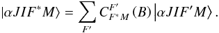 (33)It should be kept in mind that although J and F are no longer good quantum numbers, in the sense that each eigenvector now has to be decomposed over the basis vectors, the magnetic quantum numbers M and MJ = M + MI remain good quantum numbers, where MI is the magnetic quantum number for the nuclear spin and MJ is the magnetic quantum number for the total fine structure angular momentum J. Given a state |αLSJ∗IF∗M⟩, it is possible to determine the value of MJ. This is detailed in Appendix A where we provide the generalization of the previous Eqs. (30) and (31) to the case of the incomplete Paschen-Back and Back-Goudsmit effects.
4. Redistribution function in zero magnetic field
As already stated, in the absence of a magnetic field the M indexes in ΔE and ν can be replaced by the J indexes and the sums over all the M indexes can be performed.
4.1. In considering only fine structure
In the case of fine structure only and zero magnetic field, we obtain ![Mathematical equation: \begin{equation} \begin{array}{l} \medskip \mathcal{R}_{ij}\left( \nu ,\nu _{1},\vec{\Omega},\vec{\Omega}_{1}; \vec{B}=\vec{0}\right) =\dsum\limits_{J_{\rm u}J_{\rm u}^{\prime }J_{\ell }J_{\ell }^{\prime }KQ}\int f(\vec{v})\mathrm{d}^{3}\vec{v}\ (-1)^{Q}\mathcal{T} _{-Q}^{K}(j,\vec{\Omega}_{1})\mathcal{T}_{Q}^{K}(i,\vec{\Omega}) \\ \medskip\qquad \times 3\dfrac{2L_{\rm u}+1}{2S+1}(2J_{\rm u}+1)(2J_{\rm u}^{\prime }+1)(2J_{\ell }+1)(2J_{\ell }^{\prime }+1)\ (-1)^{J_{\ell }-J_{\ell }^{\prime }} \\ \medskip\qquad \times \left\{ \begin{array}{ccc} J_{\rm u} & 1 & J_{\ell } \\ L_{\ell } & S & L_{\rm u} \end{array} \right\} \left\{ \begin{array}{ccc} J_{\rm u}^{\prime } & 1 & J_{\ell } \\ L_{\ell } & S & L_{\rm u} \end{array} \right\} \left\{ \begin{array}{ccc} J_{\rm u} & 1 & J_{\ell }^{\prime } \\ L_{\ell } & S & L_{\rm u} \end{array} \right\} \left\{ \begin{array}{ccc} J_{\rm u}^{\prime } & 1 & J_{\ell }^{\prime } \\ L_{\ell } & S & L_{\rm u} \end{array} \right\} \\ \medskip\qquad \times \left\{ \begin{array}{ccc} K & J_{\rm u} & J_{\rm u}^{\prime } \\ J_{\ell } & 1 & 1 \end{array} \right\} \left\{ \begin{array}{ccc} K & J_{\rm u} & J_{\rm u}^{\prime } \\ J_{\ell }^{\prime } & 1 & 1 \end{array} \right\} \\ \medskip\qquad \times \left\{ \dfrac{\Gamma _{\rm R}}{\Gamma _{\rm R}+\Gamma _{\rm I}+\Gamma _{\rm E}+\dfrac{\mathrm{i}\Delta E_{J_{\rm u}J_{\rm u}^{\prime }}}{\hbar }}\ \delta \left( \tilde{\nu}-\tilde{\nu}_{1}-\nu _{J_{\ell }J_{\ell }^{\prime }}\right) \left[ \dfrac{1}{2}\Phi _{ba}\left( \nu _{J_{\rm u}^{\prime }J_{\ell }}-\tilde{\nu}_{1}\right) +\dfrac{1}{2}\Phi _{ba}^{\ast }\left( \nu _{J_{\rm u}J_{\ell }}-\tilde{\nu}_{1}\right) \right] \right. \\ \medskip\qquad +\left[ \dfrac{\Gamma _{\rm R}}{\Gamma _{\rm R}+\Gamma _{\rm I}+\dfrac{1}{2} \left[ D^{(K)}(\alpha _{\rm u}J_{\rm u})+D^{(K)}(\alpha _{\rm u}J_{\rm u}^{\prime })\right] + \dfrac{\mathrm{i}\Delta E_{J_{\rm u}J_{\rm u}^{\prime }}}{\hbar }}-\dfrac{\Gamma _{\rm R} }{\Gamma _{\rm R}+\Gamma _{\rm I}+\Gamma _{\rm E}+\dfrac{\mathrm{i}\Delta E_{J_{\rm u}J_{\rm u}^{\prime }}}{\hbar }}\right] \\ \medskip\qquad \times \left. \left[ \dfrac{1}{2}\Phi _{ba}\left( \nu _{J_{\rm u}^{\prime }J_{\ell }}-\tilde{\nu}_{1}\right) +\dfrac{1}{2}\Phi _{ba}^{\ast }\left( \nu _{J_{\rm u}J_{\ell }}-\tilde{\nu}_{1}\right) \right] \left[ \dfrac{1}{2}\Phi _{ba}\left( \nu _{J_{\rm u}^{\prime }J_{\ell }^{\prime }}-\tilde{\nu}\right) +\dfrac{1}{2}\Phi _{ba}^{\ast }\left( \nu _{J_{\rm u}J_{\ell }^{\prime }}-\tilde{\nu}\right) \right] \phantom{ \dfrac{\Gamma _{\rm R}}{\Gamma _{\rm R}+\Gamma _{\rm I}+\Gamma _{\rm E}+\dfrac{\mathrm{i}\Delta E_{J_{\rm u}J_{\rm u}^{\prime }}}{\hbar }}}\hspace*{-3.3cm}\right\}. \end{array} \label{eq -- redist fine zero B} \end{equation}](/articles/aa/full_html/2017/11/aa30169-16/aa30169-16-eq170.png) (34)The second branching ratio is made of two subtracted terms. In the first term,
(34)The second branching ratio is made of two subtracted terms. In the first term, ![Mathematical equation: \hbox{$\Gamma _{\rm R}+\Gamma _{\rm I}+\tfrac{1}{2}\left[ D^{(K)}(\alpha _{\rm u}J_{\rm u})+D^{(K)}(\alpha _{\rm u}J_{\rm u}^{\prime })\right] $}](/articles/aa/full_html/2017/11/aa30169-16/aa30169-16-eq171.png) is the inverse lifetime of the upper level population or coherence (alignment), which is associated with a corresponding level width by virtue of the Heisenberg uncertainty principle. In the second term and also in the first branching ratio, ΓR + ΓI + ΓE is the line width (Baranger 1958). In the presence of elastic or quasi-elastic collisions, ΓE and
is the inverse lifetime of the upper level population or coherence (alignment), which is associated with a corresponding level width by virtue of the Heisenberg uncertainty principle. In the second term and also in the first branching ratio, ΓR + ΓI + ΓE is the line width (Baranger 1958). In the presence of elastic or quasi-elastic collisions, ΓE and ![Mathematical equation: \hbox{$\tfrac{1}{2}\left[ D^{(K)}(\alpha _{\rm u}J_{\rm u})+D^{(K)}(\alpha _{\rm u}J_{\rm u}^{\prime })\right] $}](/articles/aa/full_html/2017/11/aa30169-16/aa30169-16-eq173.png) are both non-zero and are different from each other. In other words, when there are elastic or quasi-elastic collisions, the level width and line width are different. Sahal-Bréchot & Bommier (2017) develop Eq. (61) in Baranger (1958) and show that interference terms between the upper and lower level may contribute to the line width without contributing to each level width. It is the same with the purely elastic effects, in which the atom does not change Zeeman sublevel, and which contribute to ΓE but not to .
are both non-zero and are different from each other. In other words, when there are elastic or quasi-elastic collisions, the level width and line width are different. Sahal-Bréchot & Bommier (2017) develop Eq. (61) in Baranger (1958) and show that interference terms between the upper and lower level may contribute to the line width without contributing to each level width. It is the same with the purely elastic effects, in which the atom does not change Zeeman sublevel, and which contribute to ΓE but not to .
The branching ratio in line 6 of Eq. (34) can be rewritten as ![Mathematical equation: \begin{equation} \begin{array}{l} \medskip \dfrac{\Gamma _{\rm R}}{\Gamma _{\rm R}+\Gamma _{\rm I}+\dfrac{1}{2}\left[ D^{(K)}(\alpha _{\rm u}J_{\rm u})+D^{(K)}(\alpha _{\rm u}J_{\rm u}^{\prime })\right] +\dfrac{ \mathrm{i}\Delta E_{J_{\rm u}J_{\rm u}^{\prime }}}{\hbar }}-\dfrac{\Gamma _{\rm R}}{ \Gamma _{\rm R}+\Gamma _{\rm I}+\Gamma _{\rm E}+\dfrac{\mathrm{i}\Delta E_{J_{\rm u}J_{\rm u}^{\prime }}}{\hbar }}= \\ \medskip \dfrac{\Gamma _{\rm R}}{\Gamma _{\rm R}+\Gamma _{\rm I}+\dfrac{1}{2}\left[ D^{(K)}(\alpha _{\rm u}J_{\rm u})+D^{(K)}(\alpha _{\rm u}J_{\rm u}^{\prime })\right] +\dfrac{ \mathrm{i}\Delta E_{J_{\rm u}J_{\rm u}^{\prime }}}{\hbar }}\times \dfrac{\Gamma _{\rm E}- \dfrac{1}{2}\left[ D^{(K)}(\alpha _{\rm u}J_{\rm u})+D^{(K)}(\alpha _{\rm u}J_{\rm u}^{\prime })\right] }{\Gamma _{\rm R}+\Gamma _{\rm I}+\Gamma _{\rm E}+\dfrac{ \mathrm{i}\Delta E_{J_{\rm u}J_{\rm u}^{\prime }}}{\hbar }}\cdot \end{array} \end{equation}](/articles/aa/full_html/2017/11/aa30169-16/aa30169-16-eq174.png) (35)Belluzzi & Trujillo Bueno (2014), who totally ignore the depolarizing collision contribution via the D(K) coefficients, have instead (see their Eqs. (26) and (36))
(35)Belluzzi & Trujillo Bueno (2014), who totally ignore the depolarizing collision contribution via the D(K) coefficients, have instead (see their Eqs. (26) and (36)) 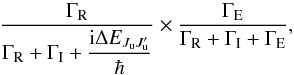 (36)which differs in the
  contribution, but coincides with ours when
  . As for the other branching ratio given in the first term of line 5 of Eq. (34), they have for this branching ratio (see their Eqs. (30) and (36))
 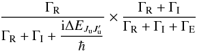 (37)while we use a different expression:
 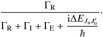 (38)Again, their branching ratio coincides with ours when . As for the product profile given in line 7 of Eq. (34), they have instead
 ![Mathematical equation: \begin{equation} \left[ \dfrac{1}{2}\Phi _{ba}\left( \nu _{J_{\rm u}J_{\ell }}-\tilde{\nu} _{1}\right) +\dfrac{1}{2}\Phi _{ba}^{\ast }\left( \nu _{J_{\rm u}J_{\ell }}- \tilde{\nu}_{1}\right) \right] \left[ \dfrac{1}{2}\Phi _{ba}\left( \nu _{J_{\rm u}^{\prime }J_{\ell }^{\prime }}-\tilde{\nu}\right) +\dfrac{1}{2}\Phi _{ba}^{\ast }\left( \nu _{J_{\rm u}J_{\ell }^{\prime }}-\tilde{\nu}\right) \right] , \end{equation}](/articles/aa/full_html/2017/11/aa30169-16/aa30169-16-eq181.png) (39)where Ju instead of is in the first profile of the formula. In addition, we would obtain a formula similar to their Eq. (26) for the Racah coefficients only in the case of an isolated Jℓ level.
(39)where Ju instead of is in the first profile of the formula. In addition, we would obtain a formula similar to their Eq. (26) for the Racah coefficients only in the case of an isolated Jℓ level.
In the collisionless regime, this redistribution function with the branching ratio (the coefficient before the δ function) is in agreement with that derived in the metalevel heuristic approach by Landi Degl’Innocenti et al. (1997), and also derived by Casini et al. (2014).
4.2. Considering also hyperfine structure
In the case of non-zero hyperfine structure and zero magnetic field, we find ![Mathematical equation: \begin{equation} \begin{array}{l} \medskip \mathcal{R}_{ij}\left( \nu ,\nu _{1},\vec{\Omega},\vec{\Omega}_{1}; \vec{B}=\vec{0}\right) =\dsum\limits_{J_{\rm u}F_{\rm u}J_{\rm u}^{\prime }F_{\rm u}^{\prime }J_{\ell }F_{\ell }J_{\ell }^{\prime }F_{\ell }^{\prime }KQ}\int f(\vec{v}) \mathrm{d}^{3}\vec{v}\ (-1)^{Q}\mathcal{T}_{-Q}^{K}(j,\vec{\Omega}_{1}) \mathcal{T}_{Q}^{K}(i,\vec{\Omega}) \\ \medskip\qquad \times 3\dfrac{2L_{\rm u}+1}{2S+1}(2J_{\rm u}+1)(2J_{\rm u}^{\prime }+1)(2J_{\ell }+1)(2J_{\ell }^{\prime }+1)(2F_{\rm u}+1)(2F_{\rm u}^{\prime }+1)(2F_{\ell }+1)(2F_{\ell }^{\prime }+1)\ (-1)^{F_{\ell }-F_{\ell }^{\prime }} \\ \medskip\qquad \times \left\{ \begin{array}{ccc} J_{\rm u} & 1 & J_{\ell } \\ L_{\ell } & S & L_{\rm u} \end{array} \right\} \left\{ \begin{array}{ccc} J_{\rm u}^{\prime } & 1 & J_{\ell } \\ L_{\ell } & S & L_{\rm u} \end{array} \right\} \left\{ \begin{array}{ccc} J_{\rm u} & 1 & J_{\ell }^{\prime } \\ L_{\ell } & S & L_{\rm u} \end{array} \right\} \left\{ \begin{array}{ccc} J_{\rm u}^{\prime } & 1 & J_{\ell }^{\prime } \\ L_{\ell } & S & L_{\rm u} \end{array} \right\} \\ \medskip\qquad \times \left\{ \begin{array}{ccc} F_{\rm u} & 1 & F_{\ell } \\ J_{\ell } & I & J_{\rm u} \end{array} \right\} \left\{ \begin{array}{ccc} F_{\rm u}^{\prime } & 1 & F_{\ell } \\ J_{\ell } & I & J_{\rm u}^{\prime } \end{array} \right\} \left\{ \begin{array}{ccc} F_{\rm u} & 1 & F_{\ell }^{\prime } \\ J_{\ell } & I & J_{\rm u} \end{array} \right\} \left\{ \begin{array}{ccc} F_{\rm u}^{\prime } & 1 & F_{\ell }^{\prime } \\ J_{\ell } & I & J_{\rm u}^{\prime } \end{array} \right\} \\ \medskip\qquad \times \left\{ \begin{array}{ccc} K & F_{\rm u} & F_{\rm u}^{\prime } \\ F_{\ell } & 1 & 1 \end{array} \right\} \left\{ \begin{array}{ccc} K & F_{\rm u} & F_{\rm u}^{\prime } \\ F_{\ell }^{\prime } & 1 & 1 \end{array} \right\} \\ \medskip\qquad \times \left\{ \dfrac{\Gamma _{\rm R}}{\Gamma _{\rm R}+\Gamma _{\rm I}+\Gamma _{\rm E}+\dfrac{\mathrm{i}\Delta E_{F_{\rm u}F_{\rm u}^{\prime }}}{\hbar }}\ \delta \left( \tilde{\nu}-\tilde{\nu}_{1}-\nu _{F_{\ell }F_{\ell }^{\prime }}\right) \left[ \dfrac{1}{2}\Phi _{ba}\left( \nu _{F_{\rm u}^{\prime }F_{\ell }}-\tilde{\nu}_{1}\right) +\dfrac{1}{2}\Phi _{ba}^{\ast }\left( \nu _{F_{\rm u}F_{\ell }}-\tilde{\nu}_{1}\right) \right] \right. \\ \medskip\qquad +\left[ \dfrac{\Gamma _{\rm R}}{\Gamma _{\rm R}+\Gamma _{\rm I}+\dfrac{1}{2} \left[ D^{(K)}(\alpha _{\rm u}F_{\rm u})+D^{(K)}(\alpha _{\rm u}F_{\rm u}^{\prime })\right] + \dfrac{\mathrm{i}\Delta E_{F_{\rm u}F_{\rm u}^{\prime }}}{\hbar }}-\dfrac{\Gamma _{\rm R} }{\Gamma _{\rm R}+\Gamma _{\rm I}+\Gamma _{\rm E}+\dfrac{\mathrm{i}\Delta E_{F_{\rm u}F_{\rm u}^{\prime }}}{\hbar }}\right] \\ \medskip\qquad \times \left. \left[ \dfrac{1}{2}\Phi _{ba}\left( \nu _{F_{\rm u}^{\prime }F_{\ell }}-\tilde{\nu}_{1}\right) +\dfrac{1}{2}\Phi _{ba}^{\ast }\left( \nu _{F_{\rm u}F_{\ell }}-\tilde{\nu}_{1}\right) \right] \left[ \dfrac{1}{2}\Phi _{ba}\left( \nu _{F_{\rm u}^{\prime }F_{\ell }^{\prime }}-\tilde{\nu}\right) +\dfrac{1}{2}\Phi _{ba}^{\ast }\left( \nu _{F_{\rm u}F_{\ell }^{\prime }}-\tilde{\nu}\right) \right] \right\}, \end{array} \end{equation}](/articles/aa/full_html/2017/11/aa30169-16/aa30169-16-eq182.png) (40)where in the energy difference
(40)where in the energy difference  each Fu quantum number stands for all the quantum numbers
  defining the Fu level. As for the depolarizing collisional rate D(K)(αuFu), αu stands for
  .
.
As stated at the end of Sect. 2, in this case it was possible to introduce the contribution of the depolarizing collisions within each fine or hyperfine structure level, via the D(K) coefficients. This was possible because in zero magnetic fields the energy differences ΔE in the branching ratios no longer depend on the Zeeman quantum numbers M, which implies that the summations over these indices can be performed. However, as stated below in greater detail, this does not completely account for the depolarizing effect of the collisions with neutral hydrogen atoms, because the depolarization is also due to the collisional transitions between the fine or hyperfine structure levels themselves, which cannot easily be taken into account in the present formalism. This requires the numerical resolution of the statistical equilibrium.
In the collisionless regime, this redistribution function with the branching ratio (the coefficient before the δ function) is in agreement with that derived in the metalevel heuristic approach by Landi Degl’Innocenti et al. (1997), and also derived by Casini et al. (2014).
5. Conclusion
In the present paper, we have given expressions for the radiation redistribution function describing both coherent and incoherent scattering in the presence of magnetic field, fine and hyperfine structure. It is found that the magnetic field (the Zeeman splitting) and the fine or hyperfine structure affect the form of the branching ratios, which weight both coherent and incoherent scattering contributions to the redistribution function. Thus, the redistribution function cannot be factorized in terms of the different contributions from individual redistributions in frequency and directions because all mechanisms – magnetic fields, fine and hyperfine structures, line profiles, velocities, and Doppler effect, spherical tensors for polarimetry – are intermingled in the redistribution function.
Since the pioneering work by Omont et al. (1972), it is well-known that the balance between the frequency coherent and incoherent contributions is dominated by the elastic collisions, which contribute to the line broadening. In a classical representation, they scramble the phase of the radiating oscillator, thus introducing finite coherence time intervals, which correspond to non-zero energy intervals via the Heisenberg uncertainty principle. But a quantitative modeling of the radiation emitted or scattered by an atom requires a quantum description. These collisions then become responsible for transitions between Zeeman sublevels. When there is no magnetic field, and all the Zeeman sublevels of a level are isoenergetic, these transitions are strictly elastic. When there is a magnetic field, these transitions are not exactly elastic. However, as the Zeeman splitting is typically very small with respect to the energy difference between the two levels connected by the emitted line, these transitions may be considered quasi-elastic. There are also quasi-elastic transitions between the fine and hyperfine structure levels of a given term. In addition, in the line broadening, there is also a contribution of collisions that do not even cause transitions. There are also interference terms that contribute to the line broadening, as noted by Sahal-Bréchot & Bommier (2014, 2017). The line broadening effect is fully accounted for via the ΓE term in the above redistribution function expressions.
In the solar atmosphere, these collisions are essentially between the emitting atom or ion and neutral hydrogen atoms, as described in Sect. 4 of Bommier (2016a). Collisions that cause transitions between levels or sublevels are responsible for depolarization. This is easily understood in the case of transitions between Zeeman sublevels of a given level. The observed linear polarization by scattering is due to imbalance between Zeeman sublevel populations. These collisions tend to equalize the sublevel populations, thus reducing the linear polarization in the scattered radiation. They are accounted for via the D(K) term (with D(0) = 0 ), which can be easily introduced in the above expressions only in the absence of a magnetic field. In the presence of a magnetic field the depolarizing effect of the transitions between Zeeman sublevels cannot be simply accounted for by this term, and there are also transitions between fine and hyperfine structure levels of a given level or term, and these transitions also contribute to depolarization. They cannot be taken into account at all in the above expressions.
All the corresponding rates, namely, transfer rates between fine or hyperfine structure levels, depolarizing rates and line broadening, are of the same order of magnitude. An example is given in the case of the Na i D1-D2 lines by Kerkeni & Bommier (2002). Numerical values of the corresponding g coefficients as functions of temperature and neutral hydrogen density are given in Eqs. (11)–(16) of that paper. It can be seen that the g1 factors, which enter the line broadening, are of the same order of magnitude as the g2 factors that are responsible for the depolarization due to transitions between Zeeman sublevels, and are also of the same order of magnitude as the g0 factors that are responsible for the transfer rates of the collisional transitions between the fine and hyperfine structure levels.
The transitions between the fine and hyperfine structure levels play a depolarizing role as important as the one of the transitions between Zeeman sublevels, but they can be accounted for only in a numerical solution of the statistical equilibrium. As an example, we numerically solved the statistical equilibrium under solar upper photosphere conditions. In 90-degree scattering, the Na i D2 linear polarization rate would be 5.5 × 10⁻³ in the absence of collisions. When all the collisional transitions are accounted for, between the Zeeman sublevels and between the fine structure levels 3p2P1/2 and 3p2P3/2, the scattered light polarization rate decreases to 2.2 × 10⁻³. When the transition rates between the fine structure levels 3p2P1/2 and 3p2P3/2 are set to zero, the scattered light polarization rate increases to 3.6 × 10⁻³. It can be concluded that the transitions between fine structure levels are as important as the transitions between Zeeman sublevels for depolarizing the emitted line.
Fully taking into account all these collisional transitions requires a numerical solution of the statistical equilibrium of the atomic levels and coherences. This is not the case for the redistribution function given above, which is based on an analytical solution of the statistical equilibrium, where in particular the transfer rates between the fine and hyperfine structure levels cannot be taken into account. The above redistribution functions thus cannot completely account for the depolarizing effect of collisions. However, such functions are widely used in radiative transfer modeling of stellar atmospheres. They ignore the lower level alignment, which also requires the numerical solution of the statistical equilibrium system of equations. In the present paper, the redistribution function derivation has been made under the unpolarized and infinitely sharp lower level approximation. An innovative numerical approach alternatively based on the numerical solution of the statistical equilibrium is currently in progress (Bommier 2016b), which enables a complete account of the collisional effects. This approach does not make use of a redistribution function.
Acknowledgments
The author is greatly indebted to the referee of this paper, Roberto Casini, for helpful suggestions that improved the quality of the manuscript.
References
- Alsina Ballester, E., Belluzzi, L., & Trujillo Bueno, J. 2016, ApJ, 831, L15 [NASA ADS] [CrossRef] [Google Scholar]
- Baranger, M. 1958, Phys. Rev., 111, 494 [NASA ADS] [CrossRef] [MathSciNet] [Google Scholar]
- Belluzzi, L., & Trujillo Bueno, J. 2012, ApJ, 750, L11 [NASA ADS] [CrossRef] [Google Scholar]
- Belluzzi, L., & Trujillo Bueno, J. 2013, ApJ, 774, L28 [NASA ADS] [CrossRef] [Google Scholar]
- Belluzzi, L., & Trujillo Bueno, J. 2014, A&A, 564, A16 [NASA ADS] [CrossRef] [EDP Sciences] [Google Scholar]
- Belluzzi, L., Trujillo Bueno, J., & Štěpán, J. 2012, ApJ, 755, L2 [NASA ADS] [CrossRef] [Google Scholar]
- Belluzzi, L., Trujillo Bueno, J., & Landi Degl’Innocenti, E. 2015, ApJ, 814, 116 [NASA ADS] [CrossRef] [Google Scholar]
- Bommier, V. 1980, A&A, 87, 109 [NASA ADS] [Google Scholar]
- Bommier, V. 1997a, A&A, 328, 706 [NASA ADS] [Google Scholar]
- Bommier, V. 1997b, A&A, 328, 726 [NASA ADS] [Google Scholar]
- Bommier, V. 2016a, A&A, 591, A59 [NASA ADS] [CrossRef] [EDP Sciences] [Google Scholar]
- Bommier, V. 2016b, A&A, 591, A60 [NASA ADS] [CrossRef] [EDP Sciences] [Google Scholar]
- Casini, R., Land iDegl’Innocenti, M., Manso Sainz, R., Landi Degl’Innocenti, E., & Landolfi, M. 2014, ApJ, 791, 94 [NASA ADS] [CrossRef] [Google Scholar]
- Casini, R., del Pino Alemán, T., & Manso Sainz, R. 2017, ApJ, 835, 114 [NASA ADS] [CrossRef] [Google Scholar]
- del Pino Alemán, T., Casini, R., & Manso Sainz, R. 2016, ApJ, 830, L24 [NASA ADS] [CrossRef] [Google Scholar]
- Hubený, I., Oxenius, J., & Simonneau, E. 1983, J. Quant. Spec. Radiat. Transf., 29, 495 [NASA ADS] [CrossRef] [Google Scholar]
- Hummer, D. G. 1962, MNRAS, 125, 21 [NASA ADS] [CrossRef] [Google Scholar]
- Kerkeni, B., & Bommier, V. 2002, A&A, 394, 707 [NASA ADS] [CrossRef] [EDP Sciences] [Google Scholar]
- Landi Degl’Innocenti, E. 1983, Sol. Phys., 85, 3 [NASA ADS] [CrossRef] [Google Scholar]
- Landi Degl’Innocenti, E. 1984, Sol. Phys., 91, 1 [NASA ADS] [CrossRef] [Google Scholar]
- Landi Degl’Innocenti, E., & Landolfi, M. 2004, Polarization in Spectral Lines (Kluwer Academic Publishers), Astrophys. Space Sci. Lib., 307 [Google Scholar]
- Landi Degl’Innocenti, E., Bommier, V., & Sahal-Bréchot, S. 1991, A&A, 244, 391 [NASA ADS] [Google Scholar]
- Landi Degl’Innocenti, E., Landi Degl’Innocenti, M., & Landolfi, M. 1997, in Forum THEMIS, La Science avec THEMIS, Science with THEMIS, eds. N. Mein, & S. Sahal-Bréchot (Observatoire de Paris-Meudon), 59 [Google Scholar]
- Mihalas, D. 1978, Stellar Atmospheres, 2nd edn. (San Francisco: Freeman & Co) [Google Scholar]
- Omont, A., Smith, E. W., & Cooper, J. 1972, ApJ, 175, 185 [NASA ADS] [CrossRef] [Google Scholar]
- Sahal-Bréchot, S., & Bommier, V. 2014, Adv. Space Res., 54, 1164 [NASA ADS] [CrossRef] [Google Scholar]
- Sahal-Bréchot, S., & Bommier, V. 2017, in Solar Polarization, ASP Conf. Ser., 8 [Google Scholar]
- Smitha, H. N., Nagendra, K. N., Sampoorna, M., & Stenflo, J. O. 2011a, A&A, 535, A35 [NASA ADS] [CrossRef] [EDP Sciences] [Google Scholar]
- Smitha, H. N., Sampoorna, M., Nagendra, K. N., & Stenflo, J. O. 2011b, ApJ, 733, 4 [NASA ADS] [CrossRef] [Google Scholar]
- Smitha, H. N., Nagendra, K. N., Stenflo, J. O., et al. 2012a, A&A, 541, A24 [NASA ADS] [CrossRef] [EDP Sciences] [Google Scholar]
- Smitha, H. N., Sowmya, K., Nagendra, K. N., Sampoorna, M., & Stenflo, J. O. 2012b, ApJ, 758, 112 [NASA ADS] [CrossRef] [Google Scholar]
- Smitha, H. N., Nagendra, K. N., Sampoorna, M., & Stenflo, J. O. 2013a, J. Quant. Spec. Radiat. Transf., 115, 46 [NASA ADS] [CrossRef] [Google Scholar]
- Smitha, H. N., Nagendra, K. N., Stenflo, J. O., & Sampoorna, M. 2013b, ApJ, 768, 163 [NASA ADS] [CrossRef] [Google Scholar]
- Smitha, H. N., Nagendra, K. N., Stenflo, J. O., Bianda, M., & Ramelli, R. 2014, ApJ, 794, 30 [NASA ADS] [CrossRef] [Google Scholar]
- Sowmya, K., Nagendra, K. N., Sampoorna, M., & Stenflo, J. O. 2014a, ApJ, 793, 71 [NASA ADS] [CrossRef] [Google Scholar]
- Sowmya, K., Nagendra, K. N., Stenflo, J. O., & Sampoorna, M. 2014b, ApJ, 786, 150 [NASA ADS] [CrossRef] [Google Scholar]
- Stenflo, J. O., & Keller, C. U. 1997, A&A, 321, 927 [NASA ADS] [Google Scholar]
- Stenflo, J. O., Gandorfer, A., & Keller, C. U. 2000a, A&A, 355, 781 [NASA ADS] [Google Scholar]
- Stenflo, J. O., Keller, C. U., & Gandorfer, A. 2000b, A&A, 355, 789 [NASA ADS] [Google Scholar]
Appendix A: Redistribution matrix in incomplete Paschen-Back effect
In this appendix, we provide the redistribution matrix in the case of incomplete Paschen-Back effect, as introduced in Sect. 3.3.
Appendix A.1: Considering only fine structure
The redistribution function is given by ![Mathematical equation: \appendix \setcounter{section}{1} \begin{equation} \begin{array}{l} \medskip \mathcal{R}_{ij}\left( \nu ,\nu _{1},\vec{\Omega},\vec{\Omega}_{1}; \vec{B}\right) =\dsum\limits_{J_{\rm u}\bar{J}_{\rm u}J_{\rm u}^{\ast }M_{\rm u}J_{\rm u}^{\prime }\bar{J}_{\rm u}^{\prime }J_{\rm u}^{\prime \ast }M_{\rm u}^{\prime }J_{\ell }\bar{J}_{\ell }J_{\ell }^{\ast }M_{\ell }J_{\ell }^{\prime }\bar{J} _{\ell }^{\prime }J_{\ell }^{\prime \ast }M_{\ell }^{\prime }KK^{\prime }Q}\int f(\vec{v})\mathrm{d}^{3}\vec{v}\ (-1)^{Q}\mathcal{T}_{-Q}^{K^{\prime }}(j,\vec{\Omega}_{1})\mathcal{T}_{Q}^{K}(i,\vec{\Omega}) \\ \medskip\qquad \times 3\dfrac{2L_{\rm u}+1}{2S+1}\sqrt{(2K+1)(2K^{\prime }+1)}\ (-1)^{M_{\ell }-M_{\ell }^{\prime }} \\ \medskip\qquad \times \sqrt{(2J_{\rm u}+1)(2\bar{J}_{\rm u}+1)(2J_{\rm u}^{\prime }+1)(2\bar{J} _{\rm u}^{\prime }+1)(2J_{\ell }+1)(2\bar{J}_{\ell }+1)(2J_{\ell }^{\prime }+1)(2 \bar{J}_{\ell }^{\prime }+1)} \\ \medskip\qquad \times C_{J_{\rm u}^{\ast }M_{\rm u}}^{J_{\rm u}}\left( B\right) C_{J_{\rm u}^{\ast }M_{\rm u}}^{\bar{J}_{\rm u}}\left( B\right) C_{J_{\rm u}^{\prime \ast }M_{\rm u}^{\prime }}^{J_{\rm u}^{\prime }}\left( B\right) C_{J_{\rm u}^{\prime \ast }M_{\rm u}^{\prime }}^{ \bar{J}_{\rm u}^{\prime }}\left( B\right) C_{J_{\ell }^{\ast }M_{\ell }}^{J_{\ell }}\left( B\right) C_{J_{\ell }^{\ast }M_{\ell }}^{\bar{J}_{\ell }}\left( B\right) C_{J_{\ell }^{\prime \ast }M_{\ell }^{\prime }}^{J_{\ell }^{\prime }}\left( B\right) C_{J_{\ell }^{\prime \ast }M_{\ell }^{\prime }}^{ \bar{J}_{\ell }^{\prime }}\left( B\right) \\ \medskip\qquad \times \left\{ \begin{array}{ccc} J_{\rm u} & 1 & J_{\ell } \\ L_{\ell } & S & L_{\rm u} \end{array} \right\} \left\{ \begin{array}{ccc} J_{\rm u}^{\prime } & 1 & \bar{J}_{\ell } \\ L_{\ell } & S & L_{\rm u} \end{array} \right\} \left\{ \begin{array}{ccc} \bar{J}_{\rm u} & 1 & J_{\ell }^{\prime } \\ L_{\ell } & S & L_{\rm u} \end{array} \right\} \left\{ \begin{array}{ccc} \bar{J}_{\rm u}^{\prime } & 1 & \bar{J}_{\ell }^{\prime } \\ L_{\ell } & S & L_{\rm u} \end{array} \right\} \\ \medskip\qquad \times \left( \begin{array}{ccc} J_{\rm u} & 1 & J_{\ell } \\ -M_{\rm u} & p & M_{\ell } \end{array} \right) \left( \begin{array}{ccc} J_{\rm u}^{\prime } & 1 & \bar{J}_{\ell } \\ -M_{\rm u}^{\prime } & p^{\prime } & M_{\ell } \end{array} \right) \left( \begin{array}{ccc} \bar{J}_{\rm u} & 1 & J_{\ell }^{\prime } \\ -M_{\rm u} & p^{\prime \prime \prime } & M_{\ell }^{\prime } \end{array} \right) \left( \begin{array}{ccc} \bar{J}_{\rm u}^{\prime } & 1 & \bar{J}_{\ell }^{\prime } \\ -M_{\rm u}^{\prime } & p^{\prime \prime } & M_{\ell }^{\prime } \end{array} \right) \\ \medskip\qquad \times \left( \begin{array}{ccc} 1 & 1 & K^{\prime } \\ -p & p^{\prime } & Q \end{array} \right) \left( \begin{array}{ccc} 1 & 1 & K \\ -p^{\prime \prime \prime } & p^{\prime \prime } & Q \end{array} \right) \\ \medskip\qquad \times \left\{ \dfrac{\Gamma _{\rm R}}{\Gamma _{\rm R}+\Gamma _{\rm I}+\Gamma _{\rm E}+\dfrac{\mathrm{i}\Delta E_{M_{\rm u}M_{\rm u}^{\prime }}}{\hbar }}\ \delta \left( \tilde{\nu}-\tilde{\nu}_{1}-\nu _{M_{\ell }M_{\ell }^{\prime }}\right) \left[ \dfrac{1}{2}\Phi _{ba}\left( \nu _{M_{\rm u}^{\prime }M_{\ell }}-\tilde{\nu}_{1}\right) +\dfrac{1}{2}\Phi _{ba}^{\ast }\left( \nu _{M_{\rm u}M_{\ell }}-\tilde{\nu}_{1}\right) \right] \right. \\ \medskip\qquad +\left[ \dfrac{\Gamma _{\rm R}}{\Gamma _{\rm R}+\Gamma _{\rm I}+\dfrac{\mathrm{i }\Delta E_{M_{\rm u}M_{\rm u}^{\prime }}}{\hbar }}-\dfrac{\Gamma _{\rm R}}{\Gamma _{\rm R}+\Gamma _{\rm I}+\Gamma _{\rm E}+\dfrac{\mathrm{i}\Delta E_{M_{\rm u}M_{\rm u}^{\prime }} }{\hbar }}\right] \\ \medskip\qquad \times \left. \left[ \dfrac{1}{2}\Phi _{ba}\left( \nu _{M_{\rm u}^{\prime }M_{\ell }}-\tilde{\nu}_{1}\right) +\dfrac{1}{2}\Phi _{ba}^{\ast }\left( \nu _{M_{\rm u}M_{\ell }}-\tilde{\nu}_{1}\right) \right] \left[ \dfrac{1}{2}\Phi _{ba}\left( \nu _{M_{\rm u}^{\prime }M_{\ell }^{\prime }}-\tilde{\nu}\right) +\dfrac{1}{2}\Phi _{ba}^{\ast }\left( \nu _{M_{\rm u}M_{\ell }^{\prime }}-\tilde{\nu}\right) \right]\phantom{ \dfrac{\Gamma _{\rm R}}{\Gamma _{\rm R}+\Gamma _{\rm I}+\Gamma _{\rm E}+\dfrac{\mathrm{i}\Delta E_{M_{\rm u}M_{\rm u}^{\prime }}}{\hbar }}}\hspace*{-3.5cm} \right\}. \end{array} \end{equation}](/articles/aa/full_html/2017/11/aa30169-16/aa30169-16-eq202.png) (A.1)
(A.1)
Appendix A.2: Considering also hyperfine structure
Given the quantum numbers in zero magnetic field  , it is possible to obtain the unique MJ quantum number of this level, from the relation
  (A.2)where min(M + I,J) is the smallest algebraic of the two quantities M + I and J, and where the minimum is taken in algebraic value taking into account the sign of M. This equation is valid if the Landé factor gJ is positive and when the level hyperfine structure has increasing F values with increasing energies. When the hyperfine structure is reversed, i.e. when when the level hyperfine structure has decreasing F values with increasing energies, always with positive gJ , the formula is instead
  (A.3)Instead, when the Landé factor gJ is negative, Eq. (A.3) applies to normal hyperfine structure and Eq. (A.2) applies to reversed hyperfine structure. Conversely, given
  in zero magnetic field, F can be retrieved following
  (A.4)for normal hyperfine structure, and
  (A.5)for reverse hyperfine structure, both for positive Landé factor gJ. For negative Landé factor gJ, Eq. (A.5) applies to normal hyperfine structure and Eq. (A.4) applies to reversed hyperfine structure.
Given these equations, it is possible to determine what decoupling weights  have to be applied, even if the fine structure J quantum number is J∗ and no longer a good quantum number. The procedure is then as follows. Given
  , it is possible to determine the corresponding MJ value as described above. Then, the weights which express the partial decoupling of the fine structure in the presence of the magnetic field, can be computed. We then denote these weights
  , in order to keep in mind that we started from . This coefficient introduces the good quantum number J′, associated with the same value of the magnetic quantum number MJ. Then, always using the above formulae, a new corresponding F value can be determined, which is denoted as F∗∗ because it is not a good quantum number, and it is different from F∗ when J′ is different from J∗. Then, the corresponding
  weights for the development over the F′ good quantum numbers can be determined, which is denoted
  to keep in mind that F∗∗ was determined from (J′IMJM).
The redistribution function is given by ![Mathematical equation: \appendix \setcounter{section}{1} \begin{equation} \begin{array}{l} \medskip \mathcal{R}_{ij}\left( \nu ,\nu _{1},\vec{\Omega},\vec{\Omega}_{1}; \vec{B}\right) =\dsum\limits_{J_{\rm u}\bar{J}_{\rm u}J_{\rm u}^{\ast }F_{\rm u}\bar{F} _{\rm u}F_{\rm u}^{\ast }M_{\rm u}J_{\rm u}^{\prime }\bar{J}_{\rm u}^{\prime }J_{\rm u}^{\prime \ast }F_{\rm u}^{\prime }\bar{F}_{\rm u}^{\prime }F_{\rm u}^{\prime \ast }M_{\rm u}^{\prime }J_{\ell }\bar{J}_{\ell }J_{\ell }^{\ast }F_{\ell }\bar{F}_{\ell }F_{\ell }^{\ast }M_{\ell }J_{\ell }^{\prime }\bar{J}_{\ell }^{\prime }J_{\ell }^{\prime \ast }F_{\ell }^{\prime }\bar{F}_{\ell }^{\prime }F_{\ell }^{\prime \ast }M_{\ell }^{\prime }KK^{\prime }Q} \\ \medskip\qquad \times \int f(\vec{v})\mathrm{d}^{3}\vec{v}\ (-1)^{Q}\mathcal{T} _{-Q}^{K^{\prime }}(j,\vec{\Omega}_{1})\mathcal{T}_{Q}^{K}(i,\vec{\Omega}) \\ \medskip\qquad \times 3\dfrac{2L_{\rm u}+1}{2S+1}\sqrt{(2K+1)(2K^{\prime }+1)}\ (-1)^{M_{\ell }-M_{\ell }^{\prime }} \\ \medskip\qquad \times \sqrt{(2J_{\rm u}+1)(2\bar{J}_{\rm u}+1)(2J_{\rm u}^{\prime }+1)(2\bar{J} _{\rm u}^{\prime }+1)(2J_{\ell }+1)(2\bar{J}_{\ell }+1)(2J_{\ell }^{\prime }+1)(2 \bar{J}_{\ell }^{\prime }+1)} \\ \medskip\qquad \times \sqrt{(2F_{\rm u}+1)(2\bar{F}_{\rm u}+1)(2F_{\rm u}^{\prime }+1)(2\bar{F} _{\rm u}^{\prime }+1)(2F_{\ell }+1)(2\bar{F}_{\ell }+1)(2F_{\ell }^{\prime }+1)(2 \bar{F}_{\ell }^{\prime }+1)} \\ \medskip\qquad \times C_{J_{\rm u}^{\ast }M_{J_{\rm u}}\left( F_{\rm u}^{\ast }M_{\rm u}\right) }^{J_{\rm u}}\left( B\right) C_{J_{\rm u}^{\ast }M_{J_{\rm u}}\left( F_{\rm u}^{\ast }M_{\rm u}\right) }^{\bar{J}_{\rm u}}\left( B\right) C_{J_{\rm u}^{\prime \ast }M_{J_{\rm u}}^{\prime }\left( F_{\rm u}^{\prime \ast }M_{\rm u}^{\prime }\right) }^{J_{\rm u}^{\prime }}\left( B\right) C_{J_{\rm u}^{\prime \ast }M_{J_{\rm u}}^{\prime }\left( F_{\rm u}^{\prime \ast }M_{\rm u}^{\prime }\right) }^{\bar{J}_{\rm u}^{\prime }}\left( B\right) \\ \medskip\qquad \times C_{J_{\ell }^{\ast }M_{J_{\ell }}\left( F_{\ell }^{\ast }M_{\ell }\right) }^{J_{\ell }}\left( B\right) C_{J_{\ell }^{\ast }M_{J_{\ell }}\left( F_{\ell }^{\ast }M_{\ell }\right) }^{\bar{J}_{\ell }}\left( B\right) C_{J_{\ell }^{\prime \ast }M_{J_{\ell }}^{\prime }\left( F_{\ell }^{\prime \ast }M_{\ell }^{\prime }\right) }^{J_{\ell }^{\prime }}\left( B\right) C_{J_{\ell }^{\prime \ast }M_{J_{\ell }}^{\prime }\left( F_{\ell }^{\prime \ast }M_{\ell }^{\prime }\right) }^{\bar{J}_{\ell }^{\prime }}\left( B\right) \\ \medskip\qquad \times C_{F_{\rm u}^{\ast \ast }\left( J_{\rm u}M_{J_{\rm u}}\right) M_{\rm u}}^{F_{\rm u}}\left( B\right) C_{\bar{F}_{\rm u}^{\ast \ast }\left( \bar{J} _{\rm u}M_{J_{\rm u}}\right) M_{\rm u}}^{\bar{F}_{\rm u}}\left( B\right) C_{F_{\rm u}^{\prime \ast \ast }\left( J_{\rm u}^{\prime }M_{J_{\rm u}}^{\prime }\right) M_{\rm u}^{\prime }}^{F_{\rm u}^{\prime }}\left( B\right) C_{\bar{F}_{\rm u}^{\prime \ast \ast }\left( \bar{J}_{\rm u}^{\prime }M_{J_{\rm u}}^{\prime }\right) M_{\rm u}^{\prime }}^{\bar{F} _{\rm u}^{\prime }}\left( B\right) \\ \medskip\qquad \times C_{F_{\ell }^{\ast \ast }\left( J_{\ell }M_{J_{\ell }}\right) M_{\ell }}^{F_{\ell }}\left( B\right) C_{\bar{F}_{\ell }^{\ast \ast }\left( \bar{J}_{\ell }M_{J_{\ell }}\right) M_{\ell }}^{\bar{F}_{\ell }}\left( B\right) C_{F_{\ell }^{\prime \ast \ast }\left( J_{\ell }^{\prime }M_{J_{\ell }}^{\prime }\right) M_{\ell }^{\prime }}^{F_{\ell }^{\prime }}\left( B\right) C_{\bar{F}_{\ell }^{\prime \ast \ast }\left( \bar{J}_{\ell }^{\prime }M_{J_{\ell }}^{\prime }\right) M_{\ell }^{\prime }}^{\bar{F} _{\ell }^{\prime }}\left( B\right) \\ \medskip\qquad \times \left\{ \begin{array}{ccc} J_{\rm u} & 1 & J_{\ell } \\ L_{\ell } & S & L_{\rm u} \end{array} \right\} \left\{ \begin{array}{ccc} J_{\rm u}^{\prime } & 1 & \bar{J}_{\ell } \\ L_{\ell } & S & L_{\rm u} \end{array} \right\} \left\{ \begin{array}{ccc} \bar{J}_{\rm u} & 1 & J_{\ell }^{\prime } \\ L_{\ell } & S & L_{\rm u} \end{array} \right\} \left\{ \begin{array}{ccc} \bar{J}_{\rm u}^{\prime } & 1 & \bar{J}_{\ell }^{\prime } \\ L_{\ell } & S & L_{\rm u} \end{array} \right\} \\ \medskip\qquad \times \left\{ \begin{array}{ccc} F_{\rm u} & 1 & F_{\ell } \\ J_{\ell } & S & J_{\rm u} \end{array} \right\} \left\{ \begin{array}{ccc} F_{\rm u}^{\prime } & 1 & \bar{F}_{\ell } \\ J_{\ell } & S & J_{\rm u} \end{array} \right\} \left\{ \begin{array}{ccc} \bar{F}_{\rm u} & 1 & F_{\ell }^{\prime } \\ J_{\ell } & S & J_{\rm u} \end{array} \right\} \left\{ \begin{array}{ccc} \bar{F}_{\rm u}^{\prime } & 1 & \bar{F}_{\ell }^{\prime } \\ J_{\ell } & S & J_{\rm u} \end{array} \right\} \\ \medskip\qquad \times \left( \begin{array}{ccc} F_{\rm u} & 1 & F_{\ell } \\ -M_{\rm u} & p & M_{\ell } \end{array} \right) \left( \begin{array}{ccc} F_{\rm u}^{\prime } & 1 & \bar{F}_{\ell } \\ -M_{\rm u}^{\prime } & p^{\prime } & M_{\ell } \end{array} \right) \left( \begin{array}{ccc} \bar{F}_{\rm u} & 1 & F_{\ell }^{\prime } \\ -M_{\rm u} & p^{\prime \prime \prime } & M_{\ell }^{\prime } \end{array} \right) \left( \begin{array}{ccc} \bar{F}_{\rm u}^{\prime } & 1 & \bar{F}_{\ell }^{\prime } \\ -M_{\rm u}^{\prime } & p^{\prime \prime } & M_{\ell }^{\prime } \end{array} \right) \\ \medskip\qquad \times \left( \begin{array}{ccc} 1 & 1 & K^{\prime } \\ -p & p^{\prime } & Q \end{array} \right) \left( \begin{array}{ccc} 1 & 1 & K \\ -p^{\prime \prime \prime } & p^{\prime \prime } & Q \end{array} \right) \\ \medskip\qquad \times \left\{ \dfrac{\Gamma _{\rm R}}{\Gamma _{\rm R}+\Gamma _{\rm I}+\Gamma _{\rm E}+\dfrac{\mathrm{i}\Delta E_{M_{\rm u}M_{\rm u}^{\prime }}}{\hbar }}\ \delta \left( \tilde{\nu}-\tilde{\nu}_{1}-\nu _{M_{\ell }M_{\ell }^{\prime }}\right) \left[ \dfrac{1}{2}\Phi _{ba}\left( \nu _{M_{\rm u}^{\prime }M_{\ell }}-\tilde{\nu}_{1}\right) +\dfrac{1}{2}\Phi _{ba}^{\ast }\left( \nu _{M_{\rm u}M_{\ell }}-\tilde{\nu}_{1}\right) \right] \right. \\ \medskip\qquad +\left[ \dfrac{\Gamma _{\rm R}}{\Gamma _{\rm R}+\Gamma _{\rm I}+\dfrac{\mathrm{i }\Delta E_{M_{\rm u}M_{\rm u}^{\prime }}}{\hbar }}-\dfrac{\Gamma _{\rm R}}{\Gamma _{\rm R}+\Gamma _{\rm I}+\Gamma _{\rm E}+\dfrac{\mathrm{i}\Delta E_{M_{\rm u}M_{\rm u}^{\prime }} }{\hbar }}\right] \\ \medskip\qquad \times \left. \left[ \dfrac{1}{2}\Phi _{ba}\left( \nu _{M_{\rm u}^{\prime }M_{\ell }}-\tilde{\nu}_{1}\right) +\dfrac{1}{2}\Phi _{ba}^{\ast }\left( \nu _{M_{\rm u}M_{\ell }}-\tilde{\nu}_{1}\right) \right] \left[ \dfrac{1}{2}\Phi _{ba}\left( \nu _{M_{\rm u}^{\prime }M_{\ell }^{\prime }}-\tilde{\nu}\right) +\dfrac{1}{2}\Phi _{ba}^{\ast }\left( \nu _{M_{\rm u}M_{\ell }^{\prime }}-\tilde{\nu}\right) \right]\phantom{\dfrac{\Gamma _{\rm R}}{\Gamma _{\rm R}+\Gamma _{\rm I}+\Gamma _{\rm E}+\dfrac{\mathrm{i}\Delta E_{M_{\rm u}M_{\rm u}^{\prime }}}{\hbar }}}\hspace*{-3.5cm} \right\}. \end{array} \end{equation}](/articles/aa/full_html/2017/11/aa30169-16/aa30169-16-eq223.png) (A.6)
(A.6)
Current usage metrics show cumulative count of Article Views (full-text article views including HTML views, PDF and ePub downloads, according to the available data) and Abstracts Views on Vision4Press platform.
Data correspond to usage on the plateform after 2015. The current usage metrics is available 48-96 hours after online publication and is updated daily on week days.
Initial download of the metrics may take a while.