| Issue |
A&A
Volume 606, October 2017
|
|
|---|---|---|
| Article Number | A127 | |
| Number of page(s) | 6 | |
| Section | Atomic, molecular, and nuclear data | |
| DOI | https://doi.org/10.1051/0004-6361/201731232 | |
| Published online | 24 October 2017 | |
Photoionization and electron impact excitation cross sections for Fe I⋆
1 Department of Physics, Western Michigan University, Kalamazoo, MI 49008, USA
e-mail: manuel.bautista@wmich.edu
2 Max Planck Institute for Astronomy, Königstuhl 17, 69117 Heidelberg, Germany
Received: 23 May 2017
Accepted: 24 July 2017
Context. Iron is a major contributor to the opacity in the atmospheres of late-type stars, as well as a major contributor to the observed lines in their visible spectrum. Iron lines are commonly used to derive basic stellar parameters from medium/high resolution spectroscopy, that is, spectroscopy which shows metal content, effective temperature, and surface gravity.
Aims. Here we present large R-matrix calculations for photoionization cross sections and electron impact collision strengths.
Methods. The photoionization calculations included 35 configurations and 134 LS close coupling terms of the target ion. The eigenfunction expansion accounts for the photoionization of the outer nl subshells, with n ≥ 4, as well as the open inner 3d subshell. Our results include total and partial (term-to-term) photoionization cross sections for 936 energy terms of iron with principal quantum number ≤10, and total angular momentum from zero to seven. Our electron impact collision strengths include the lowest 46 LS terms of the atom.
Results. The present photoionization cross sections should be considerably more accurate than those currently available in the literature. On the other hand, the electron impact cross sections, which are being reported for the first time, are needed in non-local thermodynamic equilibrium (NLTE) modeling of the solar spectrum and late-type stars in general.
Key words: atomic data / atomic processes / radiative transfer / Sun: atmosphere / stars: atmospheres
Tables 5 and 6 are only available at the CDS via anonymous ftp to cdsarc.u-strasbg.fr (130.79.128.5) or via http://cdsarc.u-strasbg.fr/viz-bin/qcat?J/A+A/606/A127
© ESO, 2017
1. Introduction
Iron is at the peak of nuclear stability among all elements, and as such is the final product of thermonuclear reactions in stellar cores (Merer 1989, and references therein). As such, iron is normally used as a proxy for the entire stellar metal content. Accurate knowledge of stellar Fe abundances is crucial for our understanding of stellar evolution as well as for the study of cosmic chemical evolution.
Neutral iron has a partly filled 3d subshell, which leads to extremely rich spectra. This and its relatively high abundance make Fe i the largest source of spectral lines in the visible spectrum of typical late-type stars and is also a major contributor to the continuum opacity. Moreover, Fe i lines are also used to derive basic stellar parameters, that is, effective temperature and surface gravity.
From the atomic physics point of view, obtaining an accurate description of Fe i is quite challenging, owing to the complexity of the effective potential acting on the 4s, 3d, and 4p electrons. In practice, the wave function of the atomic system is approximated by an anti-symmetrized product of one-electron radial functions determined from an effective potential, which for l ≥ 2 becomes a two-well potential (Karaziya 1981). The two potential wells are very different from each other, in such a way that slight variations in the potential morphology can lead to large changes in electron localization. For this reason, the atomic structure is very sensitive to orbital relaxation in electron excitation, where the magnitude of such effects varies among the different terms of a given configuration. Furthermore, finding accurate numerical solutions is very difficult and iterative self-consistent treatments, for example, the Hartree-Fock method often fails to converge or yields poor quality results. Calculations that approximate the wave functions by configuration mixing tend to become intractable, because the collapse of the electron localizations into narrow potential wells gives rise to strong electron exchange interactions. Computations that use distinct non-orthogonal orbitals for each configuration or for each LS term are very difficult due to the large number of orbitals that need to be optimized. Additional complications arise from spin-orbit coupling and relativistic corrections whose effects on calculated energy levels are comparable to the energy level separations.
Several theoretical calculations of Fe i photoionization have been reported thus far. Kelly & Ron (1972) and Kelly (1972) did the first photoionization calculation for the ground state only using a many-body perturbation method. Reilman & Manson (1979) and Verner et al. (1993) also reported on ground state cross sections, based on central field approximations. The earliest R-matrix calculation for Fe i was carried out by Sawey & Berrington (1992), but due to computational limitations these calculations included only terms dominated by the ground configuration of Fe ii, thus missing a lot of essential coupling effects. Bautista & Pradhan (1995) and Bautista (1997, B97 hereafter) did the largest R-matrix calculation possible at the time, which included 15 configurations and the lowest 52 LS terms in the close coupling expansion.
A significant advantage of R-matrix calculations over central field or many-body perturbation theory calculations is that R-matrix accounts for large numbers of correlations, often missed by other calculations, and the computed cross sections naturally include all autoionizing resonances that result from the couplings between bound and continuum states. For instance, the ground state cross section of Bautista & Pradhan (1995) was orders of magnitude greater than the central field results in the energy region just above the first ionization threshold. On the other hand, the R-matrix and many-body perturbation theory results agree well in terms of the background cross section, but the latter results miss all resonances, which contribute significantly to the photoabsorption and ionization rates.
The cross sections of B97 were adopted in many stellar atmosphere modeling codes, based on local thermodynamic equilibrium (LTE). Bell et al. (2001) found that twice the bound-free opacities from the R-matrix cross sections fit the observed solar spectrum in the 3000 and 4000 Å range reasonably well. On the other hand, Castelli & Kurucz (2004) argue that their list of autoionizing transitions, treated in the isolated resonance approximation, would be more complete than the resonance structure in the B97 cross sections and would yield enhanced opacities at around 2150 Å by 10% to 25%.
In late-type stars, various authors have tried to quantify possible departures from LTE in the formation of Fe i spectral lines, but the accuracy of NLTE models remains an issue, mostly due to the lack of complete and reliable atomic data (see Barklem 2016). The main NLTE effect on Fe i is overionization by super-thermal UV radiation fields. Under-population of Fe i levels, relative to LTE populations, arises because the mean radiation fields, at different depths in the atmosphere, differ from the Plank function for the given local temperature. This leads to over-ionization of excited levels at 2−5 eV above the ground state. Excitation balance among all Fe i levels is induced mostly through radiation-induced transitions by the non-local UV field, as well as by collisional transitions with electrons and hydrogen atoms.
In NLTE models of Fe i, it is essential that the atomic model be sufficiently large. There must be a sufficient number of excited states energetically close to the ionization threshold for collisions to couple these to the continuum and establish a realistic ionization balance. It is important to have an extensive and accurate database of radiative data, including photoionization cross sections, for this element. The size of adopted models and the magnitude of NLTE effects have varied through the years, starting with Athay & Lites (1972), who included 15 levels. Thévenin & Idiart (1999) and Collet et al. (2005) included 256 and 334 levels, respectively, and rough estimates of collisional efficiency that resulted in NLTE effects of +0.3 dex at [Fe/H] = <−3. Korn et al. (2003) included 846 states and found NLTE corrections to the Fe abundance as large as 0.45−0.55 dex for late-type metal-poor stars. By contrast, Gratton et al. (1999), using a much more incomplete Fe atom plus exceedingly efficient H I collisions, found negligible NLTE abundance corrections. Shchukina et al. (2005) performed 1.5D NLTE calculations of the Sun and HD 140283, and a 2970 states Fe atom, to find abundance corrections of only +0.07 dex for the Sun, but +0.9 dex for HD 140283. Bergemann et al. (2012) adopted a 216 level Fe i model in 1D and averaged 3D model atmospheres. They found only modest NLTE effects on the fundamental stellar parameters for cool stars, even at very low metallicities. We note that all of these work rely on the B97 photoionization cross sections and empirically calibrated excitation transitions (by hydrogen and electron impact) to match observed spectra.
Another limitation in current NLTE models is due to the absence of reliable electron impact excitation cross sections for Fe i. In this regard, Lind et al. (2017) recently modeled the center-to-limb variation of the Fe i spectrum in the Sun using 3D NLTE techniques. We showed that Fe i electron impact excitation rates are a significant source of uncertainty, after using improved photoionization and hydrogen impact cross sections. In the absence of reliable electron impact data, modelers have to resource to excitations rates estimated by simple empirical approximations, which appear to be systematically overestimated.
Given the significance of photoionization and electron impact excitation data for neutral iron in cool-stars research and the improvements in computational resources over the last two decades, we have decided to revisit the problem of Fe i photoionization and provide data of improved accuracy. In addition, we are now capable of providing electron impact excitation cross sections. These two data sets will complement new quantum mechanical calculations of excitation of Fe i by hydrogen collisions (Barklem et al., in prep.) to complete reliable NLTE models of Fe. In the next section we describe the atomic structure representation adopted here, followed by a description of the computations and the results. Our conclusions are presented in Sect. 4.
2. Photoionization cross sections
The photoionization cross sections were computed with the code RMATRX (Berrington et al. 1995). This is an implementation of the R-matrix method for atomic scattering calculations. The R-matrix method solves the Schrödinger equation for the N + 1 electron system based on a close coupling expansion of the wavefunction as  (1)where A is the antisymmetrization operator, χi are the target ion wavefunctions in the target state (SLπ)i, θj is the wavefunction for the free electron, and φj are short range correlation functions for the bound (e− + ion) system.
An accurate representation of the atomic structure of the Fe+ target is needed for the scattering calculation. For this work we use the scaled Thomas-Fermi-Dirac-Amaldi central-field potential as implemented in the computer code autostructure (Badnell 1997). Our target representation was constructed upon the one used in B97 and our more recent work on the electron impact excitation of Fe ii (Bautista et al. 2015). We adopt a 35 configuration expansion with spectroscopic orbitals 1s, 2s, 2p, 3s, 3p, 3d, 4s, 4p, 4d, 5s, 5p, 4f, 5d, 6s, and 6p. The configurations and scaling parameters for the orbitals are presented in Table 1.
autostructure configuration expansions for Fe ii.
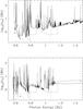 |
Fig. 1 Photoionization cross section of the 3d64s2 a 5D ground term of neutral iron. The upper panel shows the current cross section (solid line) and those of Kelly (1972; dashed line), Verner et al. (1993; dotted line), and Reilman & Manson (1979; square dots). The lower panel shows the cross section of B97 instead of the present one. |
The close coupling expansion in the present computations included the lowest 151 LS terms of the target ion, belonging to the configurations 3p63d7, 3p63d64s, 3p63d54s2, 3p63d54s4p, 3p63d54p2, 3p63d64d, 3p63d65s, and 3p63d65p. Table 2 lists all terms in the expansion.
Our R-matrix calculation resulted in the following (2S + 1) bound states with L ≤ 7 and n ≤ 10 for the Fe atom: 289 singlets, 242 triplets, 237 quintets, and 168 septets. Photoionization cross sections were computed for all bounds terms with an energy mesh of 5000 points from threshold to 1 Ry above threshold, and an additional 1000 points from 1 to 2 Ry above threshold. In addition to total photoionization cross sections, we also obtained partial cross sections, which describe ionization of every term of the Fe i to each term of the Fe ii target.
Figure 1 shows the new total photoionization cross section for the ground state of Fe and compares this with previous results. The upper panel of this figure shows the present cross section and those of Kelly (1972), Verner et al. (1993), and Reilman & Manson (1979). In the lower panel we replace the current cross section with that of B97. The calculations of Verner et al., and Reilman & Manson were based on a central-field approximation and do not account for bound-bound and bound-free correlations. These results are expected to be accurate at large photon energies (above the thresholds associate with ionization of the inner 3d subshell). It can be seen that our current cross section agrees much better with these central-field results than our previous results in B97. Our present cross section also agrees reasonably well with Kelly’s (1972) many-body perturbation theory results. Though, given the computational limitations in Kelly’s work, it could be expected to provide only an approximate cross section.
The present cross section agrees better with the central-field results at high photon energies (above 1.2 Ry) than our previous results (B97). This supports our expectation that the present results should be more accurate than in previous work. The reason why the B97 calculation underestimates the high energy cross section for the ground state is known at this point. Coupling between the target ion and the continuum must have been missing in the calculation, perhaps as a result of the truncated (N + 1)-electron expansion used in that calculation.
An interesting characteristic of the present cross section for the ground state is the dense pack of resonances for photon energies around 0.75 Ry. This feature coincides in energy with hydrogen Lyα photons and could contribute significantly to the ionization rate of neutral atoms in astronomical plasmas and planetary atmospheres.
LS terms of the target Fe ii ion included in the close coupling expansion.
Figure 2 shows the partial cross sections for photoionization of the iron a 5D ground state to the first states of the target Fe+. It can be seen that the cross section is dominated by ionization to the ground state a 6D of the target. Partial cross sections like these illustrated here are available for all terms of iron.
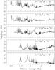 |
Fig. 2 Partial photoionization cross sections of the 3d64s2 a 5D ground term of neutral iron to specific terms of the Fe+ target. |
Figure 3 depicts the total photoionization cross sections for several excited states of Fe. The cross sections exhibit dense resonant structures that extend to higher energies than in the results of B97, owing to the present, much larger close coupling expansion. Total and partial cross sections are available for all bound states with principal quantum number up to n = 10.
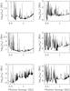 |
Fig. 3 Photoionization cross sections of the six lowest excited states of Fe. |
3. Electron impact excitation cross sections
For the calculation of collision strengths, we created a 19-configuration of the Fe atom using the autostructure atomic structure code. These configurations were formed of eight spectroscopic orbitals 1s, 2s, 2p, 3s, 3p, 3d, 4s, and 4p, and four unphysical orbitals  and
and  . The configurations and scaling parameters of our model are presented in Table 3.
autostructure configuration expansions for Fe.
We use the R-matrix scattering codes to compute electron impact collision strengths among the lowest 46 LS states of iron. Table 4 lists the terms included in the expansion. The scattering calculation includes partial waves up to L = 12, and an algebraic top-up procedure is used to estimate higher partial wave contributions to the collision strengths. The collision strengths are computed at 5000 evenly spaced energy points up to 0.5 Ry above threshold and 500 points from 0.5 to 1.0 Ry.
LS terms of iron included in the electron impact collision strengths calculation.
Figure 4 shows the collision strengths for excitation from the ground state to the lowest four excited states. We used these collision strengths to compute thermally averaged effective collision strengths  (2)where Ωij(Ej) and Ej are the collision strength and incident electron energy relative to the jth level, respectively, Te is the electron temperature, and k is the Boltzmann constant. These Maxwellian averaged effective collision strengths are presented in Table 5 (available at the CDS) for temperatures ranging from 3000 to 20 000 K. These data should be useful in NLTE modeling and abundance determinations of Fe i in late-type stars (see Lind et al. 2017; Barklem 2016).
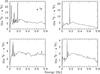 |
Fig. 4 Electron impact collision strengths in LS-coupling from the ground 4s25D term to the first four excited terms of Fe. |
4. Conclusions
We have presented extensive calculations of photoionization cross sections and collision strengths for Fe i. The computations were done in LS-coupling using the R-matrix method.
For the photoionization cross sections, we adopted a much larger close coupling expansion than in our previous work (B97). This was possible thanks to the current much larger computational resources. The new cross sections exhibit significant differences with respect to earlier results. The present results are also expected to be considerably more accurate.
Recently, we used the new cross sections to build a 463-level model of iron and used this in 3D modelling of the solar spectrum (Lind et al. 2017). The models were able to reproduce well the solar center-to-limb behavior of Fe i spectral lines. The lack of accurate electron impact excitation cross sections for Fe I is one of the remaining shortcomings in the models. Thus we have now computed these data.
To the best of our knowledge, this is the first R-matrix computation of electron impact cross sections for Fe. This calculation includes the lowest 46 terms of the atom. The cross sections were averaged over Maxwellian distributions of electron velocities. The effective collision strengths are presented for electron temperatures between 3000 K and 20 000 K. The effective collision strengths and total cross sections of this work are presented in Tables 5 and 6 available in electronic form at CDS.
References
- Badnell, N. R. 1997, J. Phys. B, 30, 1 [Google Scholar]
- Barklem, P. S. 2016, A&ARv, 24, 9 [NASA ADS] [CrossRef] [Google Scholar]
- Bautista, M. A. 1997, A&AS, 122, 167 [NASA ADS] [CrossRef] [EDP Sciences] [Google Scholar]
- Bautista, M. A., & Pradhan, A. K. 1995, J. Phys. B: At. Mol. Opt. Phys., 28, L173 [Google Scholar]
- Bell, R. A., Balachandran, S. C., & Bautista, M. 2001, ApJ, 546, L65 [NASA ADS] [CrossRef] [Google Scholar]
- Bergemann, M., Lind, K., Collet, R., Magic, Z., & Asplund, M. 2012, MNRAS, 427, 27 [NASA ADS] [CrossRef] [Google Scholar]
- Berrington, K. A., Burke, P. F., Butler, K., et al. 1997, J. Phys. B: At. Mol. Phys., 20, 6379 [Google Scholar]
- Castelli, F., & Kurucz, R. L. 2004, A&A, 419, 725 [NASA ADS] [CrossRef] [EDP Sciences] [Google Scholar]
- Kelly, H. P. 1972, Phys. Rev. A, 5, 168 [NASA ADS] [CrossRef] [Google Scholar]
- Lind, K., Amarsi, A. M., Asplund, M., et al. 2017, MNRAS, in press [Google Scholar]
- Reilman, R. F., & Manson, S. T. 1979, ApJS, 40, 815 [NASA ADS] [CrossRef] [Google Scholar]
- Verner, D. A., Yakovlev, D. G., Band, I. M., & Trzhaskovskaya, M. B. 1993, Atom. Data Nucl. Data Tables, 55, 233 [Google Scholar]
All Tables
LS terms of iron included in the electron impact collision strengths calculation.
All Figures
|
Fig. 1 Photoionization cross section of the 3d64s2 a 5D ground term of neutral iron. The upper panel shows the current cross section (solid line) and those of Kelly (1972; dashed line), Verner et al. (1993; dotted line), and Reilman & Manson (1979; square dots). The lower panel shows the cross section of B97 instead of the present one. |
| In the text | |
|
Fig. 2 Partial photoionization cross sections of the 3d64s2 a 5D ground term of neutral iron to specific terms of the Fe+ target. |
| In the text | |
|
Fig. 3 Photoionization cross sections of the six lowest excited states of Fe. |
| In the text | |
|
Fig. 4 Electron impact collision strengths in LS-coupling from the ground 4s25D term to the first four excited terms of Fe. |
| In the text | |
Current usage metrics show cumulative count of Article Views (full-text article views including HTML views, PDF and ePub downloads, according to the available data) and Abstracts Views on Vision4Press platform.
Data correspond to usage on the plateform after 2015. The current usage metrics is available 48-96 hours after online publication and is updated daily on week days.
Initial download of the metrics may take a while.