| Issue |
A&A
Volume 606, October 2017
|
|
|---|---|---|
| Article Number | A104 | |
| Number of page(s) | 13 | |
| Section | Cosmology (including clusters of galaxies) | |
| DOI | https://doi.org/10.1051/0004-6361/201730927 | |
| Published online | 20 October 2017 | |
Cosmological constraints on the neutrino mass including systematic uncertainties
1 Laboratoire de l’Accélérateur Linéaire, Univ. Paris-Sud, CNRS/IN2P3, Université Paris-Saclay, 91405 Orsay, France
e-mail: This email address is being protected from spambots. You need JavaScript enabled to view it.
2 Department of Physics and Astronomy, University of the Western Cape, Robert Sobukwe Road, 7535 Bellville, South Africa
Received: 3 April 2017
Accepted: 31 May 2017
Abstract
When combining cosmological and oscillations results to constrain the neutrino sector, the question of the propagation of systematic uncertainties is often raised. We address this issue in the context of the derivation of an upper bound on the sum of the neutrino masses (Σmν) with recent cosmological data. This work is performed within the ΛCDM model extended to Σmν, for which we advocate the use of three mass-degenerate neutrinos. We focus on the study of systematic uncertainties linked to the foregrounds modelling in cosmological microwave background (CMB) data analysis, and on the impact of the present knowledge of the reionisation optical depth. This is done through the use of different likelihoods built from Planck data. Limits on Σmν are derived with various combinations of data, including the latest baryon acoustic oscillations (BAO) and Type Ia supernovae (SNIa) results. We also discuss the impact of the preference for current CMB data for amplitudes of the gravitational lensing distortions higher than expected within the ΛCDM model, and add the Planck CMB lensing. We then derive a robust upper limit: Σmν< 0.17 eV at 95% CL, including 0.01eV of foreground systematics. We also discuss the neutrino mass repartition and show that today’s data do not allow one to disentangle normal from inverted hierarchy. The impact on the other cosmological parameters is also reported, for different assumptions on the neutrino mass repartition, and different high and low multipole CMB likelihoods.
Key words: cosmological parameters / neutrinos / methods: data analysis
© ESO, 2017
1. Introduction
In the last decade, cosmology has entered a precision era, confirming the six parameters Λ cold dark matter (CDM) concordance model with unprecedented accuracy. This allows us to open the parameters’ space, and to confront the corresponding extensions with data. In the following, we explore the neutrino sector. We only deal with three standard neutrinos species (Schael et al. 2006), and focus on the extension to the sum of the neutrino masses (Σmν). Moreover, the neutrino mass splitting scenario has been set up to match the neutrino oscillation results. A three mass-degenerate neutrinos model is advocated for and used throughout this study. It must be noted that the assumptions on the neutrino mass scenario have already been shown to be of particular importance for the derivations of cosmological results (for example in Marulli et al. 2011).
Recent works (for instance Alam et al. 2016; Sherwin et al. 2017; Giusarma et al. 2016; Yèche et al. 2017; Vagnozzi et al. 2017) on the derivation of upper bounds on Σmνusually take the cosmological microwave background (CMB) as granted. Furthermore, no uncertainty from the analysis of this cosmological probe is propagated until the final results. In this paper, we investigate the systematic uncertainties linked to the modelling of foreground residuals in the Planck CMB likelihood implementations.
To address this issue, the most accurate method would have been to make use of full end to end simulations, including an exhaustive description of the foregrounds. This is not possible given the actual knowledge of the foreground’s physical properties. Instead, we propose a comparison of the results derived from different likelihoods built from the Planck 2015 data release, and based on different foreground assumptions. Namely the public Plik and the HiLLiPOP likelihoods are examined for the high-ℓ part. We also investigate the impact of our current knowledge on the reionisation optical depth (τreio). For the low-ℓ part, the lowTEB likelihood is compared to the combination of the Commander likelihood with an auxiliary constraint on the τreio parameter, derived from the last Planck 2016 measurements (Planck Collaboration Int. XLVII 2016).
The differences of the impact of the foreground modellings are twofold: on one hand they show up as slight deviations on the Σmν bounds inferred from the different likelihoods, and, on the other hand, they manifest themselves in the form of different values of the amplitude of the gravitational lensing distortions (AL). Indeed, fitting for AL represents a direct test of the accuracy and robustness of the likelihood with respect to the ΛCDM model (Couchot et al. 2017a). We also address this point, and discuss how it is linked to Σmν.
Derivations of systematic uncertainties on Σmν are performed for different combinations of cosmological data: the Planck temperature and polarisation likelihoods, the latest BAO data from Boss DR12, and SNIa, as well as the direct measurement of the lensing distortion field power spectrum from Planck.
We also address the question of the sensitivity of the combination of those datasets to the neutrinos mass hierarchy.
We start with a description of the standard cosmology, the impact of massive neutrinos, and their mass repartition, as well as the profile likelihood method (Sect. 2). In Sect. 3, we describe the likelihoods and datasets. Turning to the Σmν constraints, we first focus on the results obtained with CMB temperature data for different likelihoods at intermediate multipoles. We investigate different choices for the low-ℓ likelihoods, and examine the pros and cons of the use of high-angular-resolution datasets. In Sect. 5, we derive the Σmν constraints obtained when combining CMB temperature, BAO and SNIa data, and check the robustness of the results with respect to the high-ℓ likelihoods. The choices for the low-ℓ parts are compared. A cross-check of the results is performed using the temperature-polarisation TE correlations. Then, the impact of the observed tension on AL is further discussed, followed by the combination of the data with the CMB lensing. The neutrino mass hierarchy question is addressed in this context. In Sect. 6.1, we discuss the (TT+TE+EE) combination with BAO and SN data, with and without CMB lensing. Finally, we derive the cosmological parameters and illustrate their variations depending on the assumptions on the neutrino mass repartition, the low-ℓ likelihoods, and the fact that we release or do not release Σmν in the fits.
2. Phenomenology and methodology
This section discusses the standard cosmology and the role of neutrinos in the Universe’s thermal history. We then briefly review the current constraints coming from the observation of the neutrino oscillations phenomenon, and discuss the mass hierarchy. A definition of the ΛCDM models considered for this paper is given. The statistical methodology based on profile likelihoods is also presented.
2.1. Standard cosmology
The “standard” cosmological model describes the evolution of a homogeneous and isotropic Universe, the geometry of which is given by the Friedman-Robertson-Walker metric, following General Relativity. In this framework, the theory reduces to the well-known Friedman equations. The Universe is assumed to be filled with several components, of different nature and evolution (matter, radiation, ...). Their inhomogeneities are accounted for as small perturbations of the metric. In the ΛCDM model, the Universe’s geometry is assumed to be Euclidean (no curvature) and its constituents are dominated today by a cosmological constant (Λ), associated with dark energy, and cold dark matter; it also includes radiation, baryonic matter and three neutrinos. Density anisotropies are assumed to result from the evolution of primordial power spectra, and only purely adiabatic scalar modes are assumed.
The minimal ΛCDM model is described with only six parameters. Two of them describe the primordial scalar mode power spectrum: the amplitude (As), and the spectral index (ns). Two other parameters represent the reduced energy densities today: ωb = Ωbh2, for the baryon, and ωc = Ωch2 for the cold dark matter. The last two parameters are the angular size of the sound horizon at decoupling, θS, and the reionisation optical depth (τreio). In this chosen parameterisation, H0 is derived in a non-trivial way from the above parameters. In addition, the sum of the neutrino masses is usually fixed to Σmν = 0.06 eV based on oscillation constraints (Forero et al. 2012, 2014; Capozzi et al. 2016): this is discussed in Sect. 2.3.
Departures from the ΛCDM model assumptions are often studied by extending its parameter space and testing it against the data, for instance, through the inclusion of Ωk for non-euclidean geometry, Neff for the number of effective relativistic species, or Yp for the primordial mass fraction of 4He during BBN. In addition to those physics-related parameters, a phenomenological parameter, AL, has been introduced (Calabrese et al. 2008a) to scale the deflection power spectrum which is used to lens the primordial CMB power spectra. This parameter permits to size the (dis-)agreement of the data with the ΛCDM lensing distortion predictions. Testing that its value, inferred from data, is compatible with one is a thorough consistency check (we refer to e.g. Calabrese et al. 2008b; Planck Collaboration XIII 2016; Couchot et al. 2017a). In this work, we use the AL consistency check in the context of the constraints on Σmν. In practice, it means that we check the value of AL (using ΛCDM+AL model) for each dataset on which we then report a Σmν limit (using νΛCDM model, i.e. with AL = 1).
2.2. Neutrinos in cosmology
One of the generic features of the standard hot big bang model is the existence of a relic cosmic neutrino background. In parallel, the observation of the neutrino oscillation phenomena requires that those particles are massive, and establishes the existence of flavour mixed-mass eigenstates (cf. Sect. 2.3; Pontecorvo 1957; Maki et al. 1962). As far as cosmology is concerned, depending on the mass of the lightest neutrino (Bilenky et al. 2001), this implies that there are at least two non-relativistic species today. Massive neutrinos therefore impact the energy densities of the Universe and its evolution.
Initially neutrinos are coupled to the primeval plasma. As the Universe cools down, they decouple from the rest of the plasma at a temperature up to a few MeV depending on their flavour (Dolgov 2002). This decoupling is fairly well approximated as an instantaneous process (Kolb & Turner 1994; Dodelson 2003). Given the fact that, with today’s observational constraints, neutrinos can be considered as relativistic at recombination (Lesgourgues & Pastor 2006). In addition, for mν in the range from 10-3 to 1 eV, they should be counted as radiation at the matter-radiation equality redshift, zeq, and as non-relativistic matter today (Lesgourgues & Pastor 2014; Lesgourgues et al. 2013), which is measured through Ωm. Σmν is therefore correlated to both zeq and Ωm.
The induced modified background evolution is reflected in the relative position and amplitude of the peaks of the CMB power spectra (through zeq). It also affects the CMB anisotropies power spectra at intermediate or high multipole (ℓ ≳ 200) as potential shifts of the power spectrum due to a change in the angular distance of the sound horizon at decoupling. Finally it also leaves an imprint on the slope of the low-ℓ tail due to the late integrated Sachs Wolfe (ISW) effect. An additional effect of massive neutrinos comes from the fact that they affect the photon temperature through the early ISW effect. As a result a reduction of the CMB temperature power spectrum below ≲ 500 is observed.
On the matter power spectrum side, two effects are induced by the massive neutrinos. In the early Universe, they free-stream out of potential wells, damping matter perturbations on scales smaller than the horizon at the non-relativistic transition. This results in a suppression of the P(k) at large k which also depends on the individual masses repartition (Hu et al. 1998; Lesgourgues & Pastor 2006). At late time, the non-relativistic neutrino masses modify the matter density, which tends to slow down the clustering.
CMB anisotropies are lensed by large-scale structures (LSS). Measuring CMB gravitational lensing therefore provides a constraint on the matter power spectrum on scales where the effects of massive neutrinos are small but still sizeable (Kaplinghat et al. 2003; Lesgourgues et al. 2006).
2.3. Neutrino mass hierarchy
As stated above, we have to choose a neutrino mass splitting scenario to define the ΛCDM model. In general, CMB data analyseis that aim at measuring cosmological parameters not related to the neutrino sector (including Planck papers, e.g. Planck Collaboration XIII 2016) are done assuming two massless neutrinos and one massive neutrino, while fixing Σmν = 0.06 eV.
For the work of this paper, our choice is motivated considering neutrino oscillation data. More precisely, we use the differences of squared neutrino masses deduced from the best fit values of the global 3ν oscillation analysis based on the work of Capozzi et al. (2016): 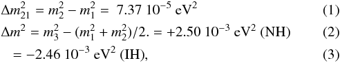 where the two usual scenarios are considered: the normal (NH) and the inverted hierarchy (IH), for which the lightest neutrino is the one of the first and third generation respectively.
 |
Fig. 1 Individual neutrino masses as a function of Σmν for the two hierarchies (NH: plain line, IH dotted lines), under the assumptions given by Eqs. (1)–(3). The vertical dahed lines outline the minimal Σmν value allowed in each case (corresponding to one massless neutrino generation). The log vertical axis prevents from the difference between m1 and m2 to be resolved in IH. |
Individual masses can be computed numerically under the above assumptions, for each mass hierarchy, as a function of Σmν, as highlighted in Fig. 1 (see also Lesgourgues & Pastor 2014). In each hierarchy, Eqs. (1)–(3) impose a lower bound on Σmν, corresponding to the case where the lightest mass is strictly null (numerically, ~0.059 and ~0.099 eV for NH and IH, respectively); also shown in Fig. 1 as vertical dashed lines.
Those results show that, given the oscillation constraints, neutrino masses are nearly degenerate for Σmν ≳ 0.25 eV. Moreover, given the current cosmological probes (essentially CMB and BAO data), we observe almost no difference in Σmν constraints when comparing results obtained with one of the two hierarchies with the case with three mass-degenerate neutrinos for which the mass repartition is such that each neutrino carries Σmν/ 3 (we refer to Sect. 5.5 and Giusarma et al. 2016; Vagnozzi et al. 2017; Schwetz et al. 2017). Indeed, as shown in Palanque-Delabrouille et al. (2015), the difference is less than 0.3% in the 3D linear matter power spectrum and is reduced even to less than 0.05% when considering the 1D flux power spectrum (see also Agarwal & Feldman 2011). This justifies the simplifying choice of the three mass-degenerate neutrinos scenario, which is used in this paper.
In Sect. 5.5, we show that this is not equivalent to the configuration where the total mass is entirely given to one massive neutrino with the two other neutrinos being massless.
2.4. Constraints on Σmν and degeneracies
The inference from CMB data of a limit on Σmνin the ΛCDM framework is not trivial because of degeneracies between parameters. Indeed, the impact of Σmν on the CMB temperature power spectrum is partly degenerated with that of some of the six other parameters.
In particular, the impact of neutrino masses on the angular-diameter distance to last scattering surface is degenerated with ΩΛ (and consequently with the derived parameters H0 and σ8) in flat models and with Ωk otherwise (Hou et al. 2014). Late-time geometric measurements help in reducing this geometric degeneracy. Indeed, at fixed θS, the BAO distance parameter DV(z) increases with increasing neutrino mass while the Hubble parameter decreases.
Another example is the correlation of Σmν with As (Allison et al. 2015). As explained in Sect 2.2, Σmν can impact the amplitude of the matter power spectrum and thus is directly correlated to As and consequently with τreio through the amplitude of the first acoustic peak (which scales like Ase− 2τreio). The constraint on Σmν therefore depends on the low-ℓ polarisation likelihood, which drives the constraints on τreio. The addition of lensing distortions, the amplitude of which is proportional to As, helps to break this degeneracy.
Moreover, the suppression of the small-scale power in LSS due to massive neutrinos, which imprints on the CMB lensing spectra, can be compensated for by an increase of the cold-dark-matter density, shifting the matter-radiation equality to early times (Hall & Challinor 2012; Pan et al. 2014). This induces an anti-correlation between Σmν and Ωcdm when using CMB observable. On the contrary, both parameters similarly affect the angular diameter distance so that BAO can help to break this degeneracy.
2.5. Cosmological model
As discussed in the previous sections, the neutrino mass repartition can have significant impact on the constraints for Σmν. By ΛCDM(1ν), we refer to the definition used in Planck Collaboration XIII (2016); it assumes two massless and one massive neutrinos.
However, in the following, we adopt a scenario with three mass-degenerate neutrinos, that is, where the neutrino generations equally share the mass (Σmν/3). We note that this is also the model adopted in Planck Collaboration XIII (2016) when Σmν constraints have been extracted. We also stick to this scenario when fixing Σmν to 0.06 eV and we refer to it as ΛCDM(3ν).
The notations νΛCDM(1ν) (resp. νΛCDM(3ν)) will be used to differentiate the case where we open the parameters’ space to Σmν from the ΛCDM(1ν) (resp. ΛCDM(3ν)) case.
To derive the values for the observables from the cosmological model, we make use of the CLASS Boltzmann solver (Blas et al. 2011). Within this software, the non-linear effects on the matter power spectrum evolution can be included using the halofit model recalibrated as proposed in Takahashi et al. (2012) and extended to massive neutrinos as described in Bird et al. (2012). Our baseline setup for the Σmν studies is to use CLASS, including non-linear effects, tuned to a high-precision setting.
In order to compare order of magnitudes in the non-linear effects propagation, we have also used CAMB (Lewis et al. 2000), in which both the Takahashi and the Mead (Mead et al. 2016) models are made available.
2.6. Profile likelihoods
The results described below were obtained from profile likelihood analyses performed with the CAMEL software1 (Henrot-Versillé et al. 2016). As described in Planck Collaboration Int. XVI (2014), this method aims at measuring a parameter θ through the maximisation of the likelihood function ℒ(θ,μ), where μ is the full set of cosmological and nuisance parameters excluding θ. For different, fixed θi values, a multidimensional minimisation of the χ2(θi,μ) = − 2lnℒ(θi,μ) function is performed. The absolute minimum,  , of the resulting
  curve is by construction the (invariant) global minimum of the problem, that is, the “best fit”. From the
  curve, the so-called profile likelihood, one can derive an estimate of θ and its associated uncertainty (James 2007). All minimisations have been performed using the MINUIT software (James 1994). In the Σmν studies presented below, 95% CL upper limits are derived following the Gaussian prescription proposed by Feldman & Cousins (1998, hereafter denoted F.C.), as described in Planck Collaboration Int. XVI (2014).
Unless otherwise explicitly stated, we use the frequentist methodology throughout this paper. A comparison with the Bayesian approach has already been presented in Planck Collaboration Int. XVI (2014) and Planck Collaboration XI (2016), showing that results do not depend on the chosen statistical method for the ΛCDM model, as well as for νΛCDM.
3. Likelihoods and datasets
In this Section, we detail the likelihoods that are used hereafter for the derivation of the results on Σmν. They are summarised in Table 1 together with their related acronyms.
Summary of data and likelihoods with their corresponding acronyms.
3.1. Planck high-ℓ likelihoods
In order to assess the impact of foreground residuals modelling on the Σmν constraints, we make use of different Planck high-ℓ likelihoods (HiLLiPOP and Plik). They both use a Gaussian approximation of the likelihood based on cross-spectra between half-mission maps at the three lowest frequencies (100, 143 and 217GHz) of Planck-HFI, but rely on different assumptions for modelling foreground residuals. Comparing the results on Σmν obtained with both of these likelihoods is a way to assess a systematic uncertainty on the foreground residuals modelling.
Plik is the public Planck likelihood. It is described in detail in Planck Collaboration XI (2016). It uses empirically motivated power spectrum templates to model residual contamination of foregrounds (including dust, CIB, tSZ, kSZ, SZxCIB and point sources) in the cross-spectra. The foreground residuals in HiLLiPOP are directly derived from Planck measurements (Couchot et al. 2017b): this is the main difference between HiLLiPOP and Plik. For ΛCDM cosmology, both likelihoods have been compared in Planck Collaboration XI (2016).
In any of the Planck high-ℓ likelihoods, the residual amplitudes of the foregrounds are compatible with expectations, with only a mild tension on unresolved point-source amplitudes coming essentially from the 100GHz frequency (we refer to Sect. 4.3 in Planck Collaboration XI 2016). In order to assess the impact of the point-source modelling on the parameter reconstructions (and in particular Σmν), we use two variants of the HiLLiPOP likelihood. The first one, labelled hlpTTps, makes use of a physical model with two unresolved point-source components, corresponding to the radio and IR frequency domains, with fixed frequency scaling factors and number counts tuned on data (Couchot et al. 2017b). The second one, labelled hlpTT, uses one free amplitude for unresolved point-sources per cross-frequency leading to six free parameters (as used in Couchot et al. 2017a), in a similar way as what is done in Plik. This allows one to alleviate the tension on the point-source amplitudes. Both hlpTTps and hlpTT lead to very similar results in the ΛCDM(1ν) model, with a lower level of correlation between parameters for the former. Comparing results obtained with hlpTTps and hlpTT is therefore useful for assessing their robustness with respect to the unresolved point-source tension.
Both HiLLiPOP and also Plik include polarisation information using the EE and TE angular cross-power spectra. Unless otherwise explicitly stated, only the temperature (TT) part is considered in the following.
Together with auxiliary constraints on nuisance parameters (such as the relative and absolute calibration) associated to each likelihood, we can also add a Gaussian constraint to the SZ template amplitudes as suggested in Planck Collaboration XI (2016). This constraint is based on a joint analysis of the Planck-2013 data with those from ACT and SPT (see Sect. 3.3) and reads:  (4)when normalized at ℓ = 3000. The role of this additional constraint is also discussed in the following.
3.2. Low-ℓ
At low-ℓ, two options are investigated to study the impact of one choice or another on the Σmν limit determination:
-
LowTEB A pixel-based likelihood that relies on thePlanck low-frequency instrument70 GHz maps for polarisation and on acomponent-separated map using all Planck frequencies fortemperature (Commander).
-
A combination of a temperature-only likelihood, Commander (Planck Collaboration XI 2016), based on a component-separated map using all Planck frequencies, and a Gaussian auxiliary constraint on the reionisation optical depth,
 derived from the last Planck results of the reionisation optical depth (Planck Collaboration Int. XLVII 2016) Lollipop likelihood (Mangilli et al. 2015).
3.3. High-resolution CMB data
High resolution CMB data, namely the ACT, SPT_high, and SPT_low datasets are also used in this work. They are later quoted “VHL” (very high-ℓ) when combined altogether. The ACT data are those presented in Das et al. (2014). They correspond to cross power spectra between the 148 and 220GHz channels built from observations performed on two different sky areas (an equatorial strip of about 300 deg2 and a southern strip of 292 deg2 for the 2008 season, and about 100 deg2 otherwise) and during several seasons (between 2007 and 2010), for multipoles between 1000 and 10000 (for 148 × 148) and 1500 to 10000 otherwise. For SPT, two distinct datasets are examined. The higher ℓ part, dubbed SPT_high, implements the results, described in Reichardt et al. (2012), from the observations of 800 deg2 at 95, 150, and 220GHz of the SPT-SZ survey. The cross-spectra cover the ℓ range between 2000 and 10000. As in Couchot et al. (2017a), we prefer not to consider the more recent data from George et al. (2015) because the calibration, based on the Planck 2013 release, leads to a 1% offset with respect to the last Planck data. We also add the Story et al. (2013) dataset, dubbed SPT_low, consisting of a 150GHz power spectrum, which ranges from ℓ = 650 to 3000, resulting from the analysis of observations of a field of 2540 deg2. Both SPT datasets have an overlap in terms of sky coverage and frequency. We have however checked that this did not bias the results by, for example, removing the 150 × 150 GHz part from the SPT_high likelihood, as was done in Couchot et al. (2017a).
3.4. Planck CMB lensing
The full sky CMB temperature and polarisation distributions are inhomogeneously affected by gravitational lensing due to large-scale structures. This is reflected in additional correlations between large and small scales, and, in particular, in a smoothing of the power spectra in TT, TE, and EE. From the reconstruction of the four-point correlation functions (Hu & Okamoto 2002), one can reconstruct the power spectrum of the lensing potential  of the lensing potential φ. In the following we make use of the corresponding 2015 temperature lensing likelihood estimated by Planck (Planck Collaboration XV 2016).
3.5. Baryon acoustic oscillations
In Sect. 5, information from the late-time evolution of the Universe geometry are also included. The more accurate and robust constraints on this epoch come from the BAO scale evolution. They bring cosmological parameter constraints that are highly complementary with those extracted from CMB, as their degeneracy directions are different.
BAO generated by acoustic waves in the primordial fluid can be accurately estimated from the two-point correlation function of galaxy surveys. In this work, we use the acoustic-scale distance ratio DV(z) /rdrag measurements from the 6dF Galaxy Survey at z = 0.1 (Beutler et al. 2014). At higher redshift, we included the BOSS DR12 BAO measurements that recently have been made available (Alam et al. 2016). They consist in constraints on (DM(z),H(z),fσ8(z)) in three redshift bins, which encompass both BOSS-LowZ and BOSS-CMASS DR11 results. Thanks to the addition of the results on fσ8(z) the constraints on Σmν are significantly reduced with respect to previous BAO measurements (Alam et al. 2016). The combination of those measurements is labelled “BAO” in the following. We note that this is an update of the BAO data with respect those used in Planck Collaboration XIII (2016).
3.6. Type Ia supernovae
SNIa also constitute a powerful cosmological probe. The study of the evolution of their apparent magnitude with redshift played a major role in the discovery of late-time acceleration of the Universe. We include the JLA compilation (Betoule et al. 2014), which spans a wide redshift range (from 0.01 to 1.2), while compiling up-to-date photometric data. This is further referenced to as “SNIa” in the following.
4. CMB temperature results
4.1. Orders of magnitude
The differences between the expected Cℓ spectra for Σmν = 0.3eV and Σmν = 0.06eV in the ΛCDM(3ν) model are shown in Fig. 2 in black on the upper panel without considering any non-linearities. The shaded area indicates the CMB spectrum divided by a factor 103. The size of the effect of increasing Σmν up to 0.3eV, except at the first peak, is of the order of ≃ 3μK2. More interesting is the bottom part of this figure (with the same color-code) where this difference is divided by the uncertainties estimated on the hlpTT spectra. It shows that a sensitivity of few percent of a σ over all the ℓ range has to be achieved in order to fit for a 0.3eV neutrino mass (the example taken here).
 |
Fig. 2 Top: absolute difference between the expected ΛCDM(3ν) TT CMB spectrum and a spectrum with the same values of the cosmological parameters except for Σmν = 0.3eV (computed with CLASS (black)) in the linear regime. The shaded area is the original ΛCDM(3ν) spectrum rescaled to 1/1000. The differences introduced by the non-linear effects for Σmν = 0.3eV are shown for CLASS in orange and CAMB in red and green (cf. text). Bottom: same differences relative to the uncertainties of the hlpTT spectrum are shown. |
The extreme case of the differences between linear and non-linear models of the CMB temperature power spectrum are also illustrated for Σmν = 0.3eV: for CLASS, in orange, corresponding to Bird et al. (2012), and for CAMB; where two models are compared, Mead in red and Takahashi in green (cf. Sect. 2). The plots show that the non-linear effects are of the order of 1μK and correspond to, at most, ≃ 1% of a σ. The difference between those estimations gives a hint towards the theoretical uncertainty associated to the propagation of non-linear effects. In addition to this, it must be kept in mind that when constraining extensions of ΛCDM models, all the cosmological parameters are correlated, such that those very small effects have to be disentangled from any other (more or less degenerated) parameter’s configuration.
To conclude, the effect one tries to fit on temperature power spectra to extract information on Σmν is very tiny, and spreads over the whole multipole range. It therefore requires one to master the underlying model used to build the CMB likelihood function to a very high accuracy.
4.2. νΛCDM(3ν)
The profile likelihood results on Σmν derived from the 2013 Planck temperature power spectra have been compared with those obtained with a Bayesian analysis in Planck Collaboration Int. XVI (2014) in the νΛCDM(1ν) model. It was then shown that the profile likelihood shape was non-parabolic. We recover the same results with the 2015 data in the νΛCDM(3ν) model: This is illustrated for different high-ℓ likelihoods combined with lowTEB on Fig. 3.
Figure 3 illustrates that the behaviour of the Δχ2 as a function of Σmν is almost independent of the choice of the likelihood. Still, the spread of the profile likelihoods gives an indication of the systematic uncertainties linked to this choice. For such particular shapes of the profile likelihood, one cannot simply use the Gaussian confidence level intervals detailed in Feldman & Cousins (1998): one should rely on extensive simulations to properly build the corresponding Neyman construction (Neyman 1937), and apply the FC ordering principle; this is beyond the scope of this work. We do not therefore quote any limit for non-parabolic profile likelihood.
The use of the ASZ constraint (cf. Eq. (4)) does improve the constraint on ΣmνThis is further discussed in Sect. 4.4, together with the impact of the combination of the VHL data.
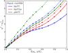 |
Fig. 3 Σmν profile likelihoods obtained with hlpTT (blue), hlpTTps (red), and PlikTT (green) combined with lowTEB(solid lines). The dashed lines include the constraint on the SZ amplitude (see Sect. 3.1). |
4.3. Impact of low-ℓ likelihoods
In Fig. 4 are shown several Σmν profile likelihoods corresponding to different choices for the low-ℓ likelihoods, while keeping hlpTT for the high-ℓ part. They all present the same shape which, as previously, prevents us from extracting upper bounds.
The results obtained when combining hlpTT with lowTEB (in blue) are very close to those obtained with a τreio auxiliary constraint+Commander (in green), showing that with those datasets, the results do not significantly depend on the choice of the low-ℓ polarisation likelihood. The same conclusion can be derived from the comparison of the results obtained using hlpTT+τreio auxiliary constraint (in red).
However, the difference between these two sets of profile likelihoods highlights the impact of Commander. A possible origin of this difference lies in the fact that when adding Commanderin ΛCDM(3ν)+AL, one reconstructs a higher AL value. Indeed, with hlpTT+τreio, we get AL = 1.16 ± 0.11, while we find AL = 1.20 ± 0.10 for hlpTT+τreio+Commander, that is, a higher value with a similar uncertainty. This higher tension with regards to the ΛCDM model (which assumes AL = 1) artificially leads to a tighter constraint on Σmν (we refer also to Sect. 5.4).
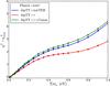 |
Fig. 4 Σmν profile likelihoods obtained with hlpTT, combined with different low-ℓ likelihoods: lowTEB, and a τreio auxiliary constraint combined or not with Commander (see text for further explanation). |
4.4. Impact of VHL data
It was suggested in Planck Collaboration XI (2016) to add a constraint on the SZ amplitudes to mimic the impact of VHL data, and we have shown in Fig. 3 that the use of such a constraint does tighten slightly the constraints on Σmν.
In this section, we try to go one step further by actually using the VHL data themselves to further constrain the foreground residuals amplitudes in the νΛCDM(3ν) case, using the same procedure as the one described in Couchot et al. (2017a).
Figure 5 shows the Σmν profile likelihoods obtained when combining hlpTT+lowTEB with VHL data in green: an apparent Δχ2 minimum shows up, around Σmν ~ 0.7, eV with a Δχ2 decrease with regards to Σmν = 0 of the order of two units. This is quite different from the Planck only Σmν profile likelihoods previously studied, even when the ASZ constraint has been added (cf. Sect. 4.2). In the νΛCDM(1ν) model, we have checked that the shape of the profile is about the same but for the minimum, which is around Σmν = 0.4 eV, close to the results obtained by Di Valentino et al. (2013), Hou et al. (2014).
To investigate this particular behaviour, we must stress that, for the combination of Planck with VHL data, one needs to compute the CMB power spectra up to ℓ ≃ 5000. We therefore need to control the foreground residuals modelling, the datasets intercalibration uncertainties, and the uncertainties on non-linear effects models over a very broad range of angular scales.
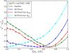 |
Fig. 5 Σmν profile likelihoods obtained for hlpTT+lowTEB+VHL built with different settings for the foregrounds: when fitting for all the foreground parameters, as usual, in green, fixing the foreground nuisance parameters to their respective expected central values (and fixing AkSZ and ASZxCIB to 0) in blue. We also report the profile likelihoods obtained when releasing one of the main foreground nuisance parameters at a time (cyan: ASZ, red: Acib). |
To tackle the issue of the foreground modelling, several settings have been studied. They are represented in Fig. 5. The blue profile likelihood is built while fixing all the foreground amplitude nuisance parameters to their mean expectation values. It can be compared with two other profile likelihoods (in cyan and in red), built when fitting only the SZ and the CIB templates amplitudes, respectively (these foregrounds dominate at the higher end of the ℓ range). The observed variations, regarding both the χ2 rise at low Σmνand the Σmν value at the minimum, with respect to the default case (in blue), show that our combination of Planck and VHL datasets is too sensitive to the foreground residuals modellings to be reliable for the derivation of a limit on Σmν. This may also come from the fact that the modelling we have used for the full sky Planck surveys is not accurate enough for the VHL small patches of the sky.
We have also investigated the impact of the uncertainties on the modelisation of non-linear effects. The mean values of the cosmological parameters, derived from the best fits of the hlpTT+lowTEB+VHL for Σmν = 0.06 eV and for 0.7 eV, were used to compute the temperature Cℓ spectra. We have observed that the difference between these spectra was of the same order of magnitude as the difference of spectra expected from two non-linear models for Σmν = 0.06 eV (namely between Takahashi and Mead cf. Sect. 2.5). As such a difference leads to a variation of up to 2 χ2 units, we could expect that the uncertainties on non-linear models would lead to similar χ2 differences2. In addition, it must be noted that this difference is also of the order of magnitude of the relative calibration between the different VHL datasets and Planck.
For all those reasons, we have chosen not to include the VHL datasets in the following (we refer also to Addison et al. 2016 for the tensions between VHL datasets and Planck). The potential impact of the uncertainties on non-linear models becomes negligible when one only considers CMB spectra up to ℓ ≃ 2500 (e.g. for Planck-only data).
5. Adding BAO and SNIa data
As noted in Sect. 2.4, the main degeneracy when using CMB data to constrain flat νΛCDM models, is between Σmν and ΩΛ which are both related to the angular-diameter distance to the last scattering surface. This translates into a degeneracy between Σmν and the derived parameters σ8 and H0 as illustrated in Fig. 6. The effect of neutrino free-streaming on structure formation favours lower σ8 values at large Σmν, which in addition require one to lower H0. Adding BAO and SNIa data breaks this relation, and substantially tightens the constraint on Σmν. In this section, we analyse the combination of Planck CMB data with DR12 BAO and SNIa data (as described in Sect. 2).
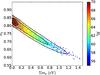 |
Fig. 6 Bayesian sampling of the hlpTTps+lowTEB posterior in the Σmν–σ8 plane, colour-coded by H0. In flat νΛCDM models, higher Σmν damps σ8, but also decreases H0. Solid black contours show one and two σ constraints from hlpTTps+lowTEB, while filled contours illustrate the results after adding BAO and SNIa data. |
5.1. hlpTT, hlpTTps, and PlikTT comparison
Figure 7 compares the three Planck likelihoods when they are combined with lowTEB, BAO and SNIa. The impressive improvement with respect to the Planck only results (Fig. 3) can be measured, for example, by the comparison of the range of Σmν values for which the Δχ2 is below 3. As expected, those results illustrate that most of the constraint on Σmν does not come from CMB-only data (at decoupling neutrinos act essentially as radiation) but from the combination with late-time probes (where they contribute as matter). In addition, for this combination of probes, the likelihood profiles take on a standard parabolic shape: the derived upper bounds on Σmν, using the F.C. prescription, are summarised in Table 2. We also quote the AL values obtained using the same datasets for the ΛCDM+AL model (fixing Σmν = 0.06eV). We note that they differ from one by roughly 2σ. The impact on the Σmν limit is discussed in Sect. 5.4.
95% CL upper limits on Σmν in νΛCDM(3ν) (i.e. with AL = 1) and results on AL (68% CL) in the ΛCDM(3ν)+AL model (i.e. with Σmν = 0.06eV) obtained when combining the Planck TT+lowTEB+BAO+SNIa.
The profiles of the different high-ℓ likelihoods are very similar, giving confidence in the final results that can be derived from their comparison. The spread between the curves reflects the remaining systematic uncertainty linked to the choice of the underlying foreground modelling. We have checked that, for hlpTT and hlpTTps, removing the foreground nuisance parameter auxiliary constraints does not impact the results: this provides an additional proof that the model and the data are in very good agreement. The information added by the ASZ constraint is of no use in this particular combination of data within the νΛCDM(3ν) model. The systematic uncertainty on the Σmν limit due the foreground modelling, deduced from this comparison, is therefore estimated to be of the order of 0.03 eV for this particular data combination.
As expected, the main improvement with respect to the Planck only case comes from the addition of the BAO dataset: the contribution on the Σmν limit of the addition of SNIa is of the order of ≃ 0.01 eV.
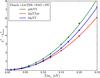 |
Fig. 7 Σmν profile likelihoods derived for the combination of lowTEB, various Planck high-ℓ likelihoods, BAO and SNIa: a comparison is made between hlpTT, hlpTTps, and PlikTT. |
5.2. Impact of low-ℓ likelihoods
While in the previous Section we focused on the estimation of the remaining systematic uncertainties linked to the choice of the high-ℓ likelihood, a comparison of the low-ℓ parts is now performed. We already discussed in Sect. 4.3 the impact of this choice on the results derived from CMB data only; this comparison focuses on the combination of BAO and SNIa data.
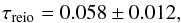
The results are summarised in Fig. 8. For the two HiLLiPOP likelihoods, tightening the constraints on τreio with the use of τreio+Commander in place of lowTEBresults in a limit of 0.15eV (resp. 0.16eV) for hlpTTps (resp. hlpTT) and amounts to a few 10-2eV decrease compared to the lowTEB case. This decrease is a direct consequence of both the (Σmν,τreio) correlation (Allison et al. 2015), and the smaller value of the reionisation optical depth constraint from ~0.07 to 0.058 (Planck Collaboration Int. XLVII 2016).
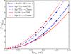 |
Fig. 8 Σmν profile likelihoods derived for the combination of Planck high-ℓ likelihoods (hlpTT and hlpTTps) with BAO and SNIa, and either lowTEB or the τ auxiliary constraint at low-ℓ. |
5.3. Cross-check with TE
As pointed out in Galli et al. (2014) and Couchot et al. (2017b), CMB temperature-polarisation cross-correlations (TE) give competitive constraints on ΛCDM parameters. The leading advantage of using only these data is that one depends very weakly on foreground residuals and therefore uncertainty linked to the model parametrisation is reduced. In practice, only one foreground nuisance parameter is required: the amplitude of the polarized dust. Nevertheless, the signal-to-noise ratio being lower than in the TT case for Planck, a likelihood based on TE spectra is not competitive when constraining extensions to the six ΛCDM parameters. Indeed an estimation of the TE-only constraint on Σmν would lead to a limit higher than 1eV. However, as soon as BAO data are added, one obtains a constraint competitive with TT as shown in Fig. 9. As in the TT case, all profile likelihoods are nicely parabolic, and the corresponding limits are summarised in Table 3.
95% CL upper limits on Σmν in νΛCDM(3ν) obtained with hlpTE+BAO+SNIa in combination with lowTEB, or an auxiliary constraint on τreio and Commander.
As for temperature-only data, adding the SNIa data improves only very marginally the results up to 0.01 eV. Tests of the dependencies on the low-ℓ likelihoods have also been performed and an example is given in Table 3. As a final result, we obtain Σmν < 0.20 eV at 95% CL as strong as in the TT case, showing that the loss in signal over noise of TE (statistical uncertainty) is balanced by improved control of foreground modelling (systematic uncertainty).
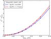 |
Fig. 9 Σmν profile likelihoods obtained when combining hlpTE with either lowTEB (red), or an auxiliary constraint on τreio+Commander (blue) and with BAO and SNIa. |
5.4. AL and Σmν
5.4.1. νΛCDM(3ν) model
As previously stated, CMB data tend to favour a value of AL greater than one. In the combination of Planck high-ℓ likelihood with lowTEB, BAO and SNIa, the AL values estimated in the ΛCDM(3ν)+AL model, are summarised in the third column of Table 2. As expected they are almost identical to the ones obtained with CMB data only.
The fact that AL is not fully compatible with the ΛCDM model, has to be taken into account when stating final statements on Σmν since, otherwise, the results are not obtained within a coherent model: on one side we fix AL to one by working within a νΛCDM model while the data are, at least, ≃ 2σ away from this value, and on the other side, fixing AL = 1 results, artificially, in a tighter constraint on Σmν. This last effect can be seen, for example, in Table 2, for which the higher the AL value, the tighter the constraint on Σmν.
There are two ways to propagate this effect on the Σmν limit determination. The first is to open up the parameter space to νΛCDM(3ν)+AL (as it is done in the Sect. 5.4.2). The second is to better constrain the lensing sector by considering the Planck lensing likelihood and then to fit only for the Σmν extension using the νΛCDM(3ν) model, fixing AL = 1 (cf. Sect. 5.4.3).
5.4.2. The νΛCDM+ AL model
In this Section, we open the νΛCDM(3ν) parameter space to AL for the combination of Planck high-ℓ likelihoods with lowTEB+BAO+SNIa.
The limits derived from the corresponding profile likelihoods are summarised in Table 4. The increase of the limits with respect to those of Table 2 results from two effects. First of all we open up the parameter space, propagating the uncertainty on AL on the Σmν determination. The second effect is linked to the fact that, as already stated, the CMB data tend to favour a higher AL value than expected within a ΛCDM model. We have observed that this effect propagates as an increase of the baryon energy density, a slight decrease of the cold dark matter energy density, and this shows up, with a fixed geometry, as a higher neutrino energy density. Those two combined effects drive the limit to high values of Σmν when fitting for both Σmν and AL.
Results on Σmν (95% CL upper limits) and AL (68% CL) obtained from a combined fit in the νΛCDM(3ν)+AL model with Planck TT+lowTEB+BAO+SNIa.
5.4.3. Combining with CMB lensing
Another way of tackling the AL problem is to add the lensing Planck likelihood to the combination (see Sect. 3.4). This allows us to obtain a lower AL value, as shown in the third column of Table 5 in the ΛCDM(3ν)+AL model. With this combination, the AL value extracted from the data is fully compatible with the ΛCDM model, allowing us to derive a limit on Σmν together with a coherent AL value.
As expected, in the ΛCDM(3ν) model, the Σmν limits are therefore pushed toward higher values than what has been presented in Table 2: this is exemplified by the second column of Table 5.
95% CL upper limits on Σmν in νΛCDM(3ν) (i.e. with AL = 1) and results on AL (68% CL) in the ΛCDM(3ν)+AL model (i.e. with Σmν = 0.06eV) obtained when combining Planck TT+lowTEB+BAO+SNIa+lensing.
5.5. Constraint on the neutrino mass hierarchy
As explained in Sect. 2.4, the neutrino mass repartition leaves a very small signature on the CMB and matter power spectra. In this section, we test whether or not the combination of modern cosmological data is sensitive to it.
We compare the results obtained with four configurations of neutrino mass settings. The first one corresponds to one massive and two massless neutrinos as in νΛCDM(1ν) and is labelled [ 1ν ]. The second one is built under the assumption of three mass-degenerate neutrinos as in νΛCDM(3ν) and is denoted [ 3ν ]. We also discuss the normal hierarchy [3ν NH] (resp. inverted hierarchy [3ν IH]) derived from Eqs. (1) and (2) (resp. Eq. (3)).
In contrast with the rest of this paper, we did not subtract, in this Section, the minimum of the χ2 to plot the profile likelihoods. This allows us to assess the χ2 difference between the various neutrino configurations. In Fig. 10, we show the results obtained using the combination hlpTT+ lowTEB+BAO+SNIa+lensing. The 95% CL upper limits derived from these profile likelihoods are reported in Table 6.
The observed difference between [1ν] and [3ν] illustrates the impact of the choice of the number of massive neutrinos on the derived constraint on Σmν. More important is the comparison of the profile likelihoods built for the different hierarchy scenarios. The fact that they are indistinguishable (both in shape and in absolute χ2 values), and, even more, that they are almost identical to the one of the three degenerated masses, shows that there is, with modern data, no hint of a preference for the data towards one scenario or another, for this particular data combination (we refer also to the latest discussion in Schwetz et al. 2017).
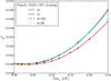 |
Fig. 10 Profiled χ2 on Σmν derived for the combination hlpTT+lowTEB+BAO+SNIa+lensing in the one massive, two massless scenario (red), in the degenerate masses hypothesis (green), and for normal (NH, dashed blue line) and inverse (IH, dashed cyan line) hierarchies. |
95% CL upper limits on Σmν obtained with hlpTT+lowTEB+BAO+SNIa+lensing for different neutrino mass repartition: three degenerate masses, normal hierarchy (NH), inverse hierarchy (IH) and one massive plus two massless neutrinos.
95% CL upper limits on Σmν in νΛCDM(3ν) obtained when combining PlikALL, hlpALL or hlpALLps with lowTEB+SNIa+BAO. ALL refers to the combination TT+TE+EE.
6. Adding CMB polarisation
In the previous Section, we derived limits on Σmν from various high-ℓPlanck temperature likelihoods combined with BAO and SNIa. All those results were cross-checked with the almost foreground-free TE Planck spectra. In this section, we combine the temperature and polarisation CMB data from Planck together with BAO, SNIa. As done previously, the CMB lensing is then also added in the combination to address the AL tension. We then show the final results of this paper on the Σmν determination.
6.1. Combination of TT, TE, EE BAO and SNIa
The 95% CL upper limits on Σmν corresponding to the full TT+TE+EE likelihoods (labelled ALL), combined with BAO, SNIa and lowTEB are summarised in Table 7.
They are very close to the temperature-only upper limit of Table 2, showing that the use of the polarisation information in addition to the temperature does not add much information. They are also very close, showing the consistency of the results with respect to the high-ℓPlanck likelihoods when BAO and SNIa are included.
However, for this data combination, we are still left with a 2σ tension on AL (the AL values are almost the same as the ones of the TT combination of Table 2). The fact that the results from PlikALL are lower than those of HiLLiPOP is linked to the fact that the AL value of Plik is higher than the one of HiLLiPOP. We will come back to this point in the next section.
6.2. Combining with CMB lensing
As done in Sect. 5.4.3, we now add to the data combination, the lensing Planck likelihood (see Sect. 3.4). The corresponding profile likelihoods are shown in Fig. 11, and the results are given in Table 8 for νΛCDM(3ν) (i.e. with AL = 1). To compare with Table 7, the Σmν limits are higher when lowTEB is used at low-ℓ, but more robust with respect to the AL issue thanks to the use of the lensing data. For the ALL case, in the ΛCDM(3ν)+AL model we end up with a value of AL compatible with one and very comparable with those of Table 5. The limits on Σmν are therefore not artificially lowered by an overly high AL value. Even though we end up with upper limits that are pushed toward higher bounds if compared to those obtained without the lensing data, we insist on the fact that this data combination is compatible with the ΛCDM model.
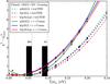 |
Fig. 11 Σmν profile likelihoods obtained when combining either PlikALL, hlpALL, and hlpALLps, temperature+polarisation likelihoods, with the CMB lensing likelihood, BAO and SNIa for lowTEB and for the combination of an auxiliary constraint on τ+Commander. We also materialise the minimal neutrino masses for the normal and inverted hierarchy inferred from neutrino oscillation measurements. |
95% CL upper limits on Σmν in νΛCDM(3ν) obtained when combining PlikALL, hlpALL or hlpALLps with SNIa+BAO+lensing, using lowTEB for the low-ℓ (second column) and for the combination of an auxiliary constraint on τreio+Commander (third column).
When making use of the latest τreio measurement, we almost recover the results of Table 7. We use the differences between the upper limits obtained with the three Planck likelihoods of Table 8 (last column) to estimate a systematic error coming from the foreground modelling of 0.01eV.
Table 9 provides the χ2 = − 2log ℒ values as a function of Σmν, where the likelihood (ℒ) has been profiled out over the nuisance and cosmological parameters. It corresponds to the combination of hlpALLps+BAO+SNIa+lensing, using the auxiliary constraint on τreio combined with Commander at low-ℓ. This dataset is chosen for the final limits derivation since it corresponds to the most up-to-date results on τreio. Table 9 can be used for neutrino global fits.
Values of the χ2 = − 2log ℒ profiled out over all the other (cosmological and nuisance) parameters as a function of Σmν for the hlpALLps+BAO+SNIa+lensing combination, using the auxiliary constraint on τreio combined with Commander at low ℓ.
 |
Fig. 12 Comparison of various estimations of cosmological parameters, together with their 68% CL, in the ΛCDM(3ν), νΛCDM(3ν) and ΛCDM(1ν) models, from the combination of: the high-ℓPlanck (hlpALL, hlpALLps or PlikALL separated by the vertical dashed lines); the lowTEB likelihood or a τreio auxiliary constraint; Commander; the CMB lensing from Planck; BAO; and SNIa. Those results, derived from profile likelihood analyses, are compared (last point in black) to the Planck 2015 results with a similar data combination (last column of Table 4, in Planck Collaboration XIII 2016). |
6.3. Cosmological parameters: ΛCDM versus νΛCDM
We compare the ΛCDM cosmological parameters and their error bars derived with the profile likelihood method using various combinations of CMB temperature+polarisation high-ℓ and low-ℓ likelihoods, with the CMB lensing likelihood from Planck, BAO and SNIa datasets.
More precisely, this comparison is done:
-
1.
when Σmν is, or not, a free parameter;
-
2.
using different foreground-modelling choices (via the different high-ℓ likelihoods);
-
switching from the publicly available lowTEB low-ℓ likelihood to the combination of an auxiliary constraint on τreio with Commander, to size the impact of a tighter constraint on τreio;
-
4.
between the neutrino mass settings of the ΛCDM(1ν) and ΛCDM(3ν) models.
These results are summarised in Fig. 12. They are very similar to the Planck 2015 results (Planck Collaboration XIII 2016) even though we are using here a new version of the BAO data (DR12). As stated in Sect. 2.6, we have checked that they do not depend on the chosen statistical approach (Bayesian or Frequentist), either for the ΛCDM or for the νΛCDM model.
The values and uncertainties of the cosmological parameters in the νΛCDM(3ν) model (in red) are similar to those obtained in ΛCDM(3ν) (in blue), but are marginally shifted and with slightly larger 68% CL uncertainties. This is true with lowTEB (as seen from the hlpALL results, circles) as well as with an auxiliary constraint on τreio with Commander for both hlpALL and hlpALLps (shown with squares). The increase of the uncertainties is related to the addition of Σmν in the fit. The small shifts of the mean values are nearly the same for all the tested cases. This could be the result of a best fit value of Σmν slightly different from 0.06 eVassumed in the ΛCDM(3ν) model.
Switching from lowTEB (plain line in Fig. 12) to an auxiliary constraint on τreio + Commander (dotted lines) at low-ℓ changes the results on τreio and As and reduces their uncertainties, as expected. We observe small shifts on other parameters (ωb, ωcdm, ns), consistently for all three high-ℓ likelihoods, when fitting for Σmν. They result from intrinsic correlations between (τreio, As) and the other cosmological parameters.
In the six-parameter ΛCDM(3ν) case, hlpALL and hlpALLps give very similar results, but for a small difference on ns. This is related to the more constraining point source model (we refer to the discussion in Couchot et al. 2017b). The comparison, illustrated in Fig 12, shows the robustness of the cosmological parameters estimation with respect to the choice of the CMB (high-ℓ and low-ℓ) likelihoods. The residual (small) differences between them illustrate the remaining systematic uncertainties. For example, the differences between Plik and HiLLiPOPcould be linked to the different choices made for masks, ℓ ranges and foreground templates used in both cases.
Finally, the values and uncertainties of the cosmological parameters fitted in the ΛCDM(3ν) and ΛCDM(1ν), with PlikALL, are very close to each other. This shows that the mass repartition has almost no effect on ΛCDM parameters when Σmν is fixed to 0.06 eV.
7. Conclusions
We have addressed the question of the propagation of foreground systematics on the determination of the sum of the neutrino masses through an extensive comparison of results derived from the combination of cosmological data including Planck CMB likelihoods with different foreground modelisations.
For this comparison we have worked within the νΛCDM(3ν) model assuming three mass-degenerate neutrinos, motivated by oscillations results. We have justified this approximation, showing that it leads to the same results as those obtained when considering normal or inverted hierarchy.
We have shown that the details of the foreground residuals modelling play a non-negligible role in the Σmν determination, and affect the results in two different ways. Firstly, they are unveiled by different AL values for the various likelihoods, up to 2σ away from ΛCDM. This impacts the Σmν limit: the higher the AL value favoured by the data, the lower the upper bound on Σmν. For this reason we have added the CMB lensing in the combination of data, providing a way to derive a limit with an AL value fully compatible with the ΛCDM model. Secondly, it introduces a spread of the profile likelihoods, resulting in various limits on Σmν, from which a systematic uncertainty was derived. We have compared CMB temperature and polarisation results, as well as their combination, and showed that the results are very consistent between themselves.
We have also discussed the impact of the low-ℓ likelihoods. We have shown, through the use of an auxiliary constraint on τreio (derived from the latest Planck reionisation results) combined with Commander, that a better determination of the uncertainty on τreio led to a reduction of the upper limit on Σmν, of the order of a few 10-2 eV with respect to the lowTEB case.
We have also addressed the question of the neutrino hierarchy. We have shown that the profile likelihoods are identical in the normal and inverted hierarchies, proving that the current data are not sensitive to the details of the mass repartition. Still, cosmological data could rule out the inverted hierarchy if they lead to a low-enough Σmν limit. However, today, the Σmν upper bound is still too high to get to this conclusion.
Combining the latest results from CMB anisotropies with Planck (both in temperature and polarisation, and including the last measurement of τreio), with BAO, SNIa, and the CMB lensing, we end up with: ![Mathematical equation: \begin{eqnarray} \mnu<\ 0.17\ [ \hbox{incl.}\ 0.01\ \hbox{(foreground syst.)} ] \hbox{\ eV\ at\ }95\%\hbox{\ CL} .\nonumber \end{eqnarray}](/articles/aa/full_html/2017/10/aa30927-17/aa30927-17-eq144.png) The values of the χ2 of the profile likelihoods are also given for further use in neutrinos global fits. For the first time, all the following effects have been taken into account:
The values of the χ2 of the profile likelihoods are also given for further use in neutrinos global fits. For the first time, all the following effects have been taken into account:
-
systematic variations related to foreground modelling error;
-
a value of AL compatible with expectations;
-
a lower value for τreio compatible with the latest measurements from Planck;
-
the new version of the BAO data (DR12),
making our final Σmν limit a robust result. For all these reasons, we think that this is the lowest upper limit we can obtain today using cosmological data.
As far as cosmology is concerned, the uncertainty on the neutrino mass will be improved in the future: it could be reduced by a factor ≃ 5 if one refers, for instance, to the forecasts on the combination of next-generation “Stage 4” B-mode CMB experiments with BAO and clustering measurements from DESI (Audren et al. 2013; Font-Ribera et al. 2014; Allison et al. 2015; Abazajian et al. 2016; Archidiacono et al. 2017). Nevertheless, the proper propagation of systematics, in particular coming from the modelling of foregrounds, is a more important topic than ever in today’s cosmology.
Still, the proper propagation of the uncertainties of non-linear effects is beyond the scope of this work.
Acknowledgments
We gratefully acknowledge the IN2P3 Computer Center (http://cc.in2p3.fr) for providing the computing resources and services needed to this work.
References
- Abazajian, K. N., Adshead, P., Ahmed, Z., et al. 2016, ArXiv e-prints [arXiv:1610.02743] [Google Scholar]
- Addison, G. E., Huang, Y., Watts, D. J., et al. 2016, ApJ, 818, 132 [NASA ADS] [CrossRef] [Google Scholar]
- Agarwal, S., & Feldman, H. A. 2011, MNRAS, 410, 1647 [NASA ADS] [Google Scholar]
- Alam, S., Ata, M., Bailey, S., et al. 2016, MNRAS, 470, 2617 [Google Scholar]
- Allison, R., Caucal, P., Calabrese, E., Dunkley, J., & Louis, T. 2015, Phys. Rev. D, 92, 123535 [NASA ADS] [CrossRef] [Google Scholar]
- Archidiacono, M., Brinckmann, T., Lesgourgues, J., & Poulin, V. 2017, J. Cosmol. Astropart. Phys., 1702, 052 [NASA ADS] [CrossRef] [Google Scholar]
- Audren, B., Lesgourgues, J., Bird, S., Haehnelt, M. G., & Viel, M. 2013, J. Cosmol. Astropart. Phys., 1301, 026 [NASA ADS] [CrossRef] [Google Scholar]
- Betoule, M., Kessler, R., Guy, J., et al. 2014, A&A, 568, A22 [NASA ADS] [CrossRef] [EDP Sciences] [Google Scholar]
- Beutler, F., Saito, S., Brownstein, J., et al. 2014, MNRAS, 444, 3501 [NASA ADS] [CrossRef] [Google Scholar]
- Bilenky, S. M., Pascoli, S., & Petcov, S. T. 2001, Phys. Rev. D, 64, 053010 [CrossRef] [Google Scholar]
- Bird, S., Viel, M., & Haehnelt, M. G. 2012, MNRAS, 420, 2551 [NASA ADS] [CrossRef] [Google Scholar]
- Blas, D., Lesgourgues, J., & Tram, T. 2011, J. Cosmol. Astropart. Phys., 7, 034 [Google Scholar]
- Calabrese, E., Slosar, A., Melchiorri, A., Smoot, G. F., & Zahn, O. 2008a, Phys. Rev. D, 77, 123531 [NASA ADS] [CrossRef] [Google Scholar]
- Calabrese, E., Slosar, A., Melchiorri, A., Smoot, G. F., & Zahn, O. 2008b, Phys. Rev. D, 77, 123531 [NASA ADS] [CrossRef] [Google Scholar]
- Capozzi, F., Lisi, E., Marrone, A., Montanino, D., & Palazzo, A. 2016, Nucl. Phys. B, 908, 218 [NASA ADS] [CrossRef] [Google Scholar]
- Couchot, F., Henrot-Versillé, S., Perdereau, O., et al. 2017a, A&A, 597, A126 [NASA ADS] [CrossRef] [EDP Sciences] [Google Scholar]
- Couchot, F., Henrot-Versillé, S., Perdereau, O., et al. 2017b, A&A, 602, A41 [NASA ADS] [CrossRef] [EDP Sciences] [Google Scholar]
- Das, S., Louis, T., Nolta, M. R., et al. 2014, J. Cosmol. Astropart. Phys., 4, 14 [NASA ADS] [CrossRef] [Google Scholar]
- Di Valentino, E., Galli, S., Lattanzi, M., et al. 2013, Phys. Rev. D, 88, 023501 [NASA ADS] [CrossRef] [Google Scholar]
- Dodelson, S. 2003, Modern Cosmology (San Diego: Academic Press) [Google Scholar]
- Dolgov, A. D. 2002, Phys. Rept., 370, 333 [CrossRef] [Google Scholar]
- Feldman, G. J., & Cousins, R. D. 1998, Phys. Rev. D, 57, 3873 [Google Scholar]
- Font-Ribera, A., McDonald, P., Mostek, N., et al. 2014, J. Cosmol. Astropart. Phys., 1405, 023 [Google Scholar]
- Forero, D. V., Tortola, M., & Valle, J. W. F. 2012, Phys. Rev. D, 86, 073012 [NASA ADS] [CrossRef] [Google Scholar]
- Forero, D. V., Tortola, M., & Valle, J. W. F. 2014, Phys. Rev. D, 90, 093006 [NASA ADS] [CrossRef] [Google Scholar]
- Galli, S., Benabed, K., Bouchet, F., et al. 2014, Phys. Rev. D, 90, 063504 [NASA ADS] [CrossRef] [Google Scholar]
- George, E. M., Reichardt, C. L., Aird, K. A., et al. 2015, ApJ, 799, 177 [Google Scholar]
- Giusarma, E., Gerbino, M., Mena, O., et al. 2016, Phys. Rev. D, 94, 083522 [NASA ADS] [CrossRef] [Google Scholar]
- Hall, A. C., & Challinor, A. 2012, MNRAS, 425, 1170 [NASA ADS] [CrossRef] [Google Scholar]
- Henrot-Versillé, S., Perdereau, O., Plaszczynski, S., et al. 2016, ArXiv e-prints [arXiv:1607.02964] [Google Scholar]
- Hou, Z., Reichardt, C. L., Story, K. T., et al. 2014, ApJ, 782, 74 [NASA ADS] [CrossRef] [Google Scholar]
- Hu, W., & Okamoto, T. 2002, ApJ, 574, 566 [Google Scholar]
- Hu, W., Eisenstein, D. J., & Tegmark, M. 1998, Phys. Rev. Lett., 80, 5255 [NASA ADS] [CrossRef] [Google Scholar]
- James, F. 1994, MINUIT Function Minimization and Error Analysis: Reference Manual Version 94.1 [Google Scholar]
- James, F. 2007, Statistical Methods in Experimental Physics (World Scientific) [Google Scholar]
- Kaplinghat, M., Knox, L., & Song, Y.-S. 2003, Phys. Rev. Lett., 91, 241301 [NASA ADS] [CrossRef] [PubMed] [Google Scholar]
- Kolb, E., & Turner, M. 1994, The Early Universe, Frontiers in Physics (Avalon Publishing) [Google Scholar]
- Lesgourgues, J., & Pastor, S. 2006, Phys. Rept., 429, 307 [NASA ADS] [CrossRef] [Google Scholar]
- Lesgourgues, J., & Pastor, S. 2014, New J. Phys., 16, 065002 [NASA ADS] [CrossRef] [Google Scholar]
- Lesgourgues, J., Perotto, L., Pastor, S., & Piat, M. 2006, Phys. Rev. D, 73, 045021 [NASA ADS] [CrossRef] [Google Scholar]
- Lesgourgues, J., Mangano, G., Miele, G., & Pastor, S. 2013, Neutrino Cosmology (Cambridge: Cambridge Univ. Press) [Google Scholar]
- Lewis, A., Challinor, A., & Lasenby, A. 2000, ApJ, 538, 473 [Google Scholar]
- Maki, Z., Nakagawa, M., & Sakata, S. 1962, Prog. Theor. Phys., 28, 870 [NASA ADS] [CrossRef] [MathSciNet] [Google Scholar]
- Mangilli, A., Plaszczynski, S., & Tristram, M. 2015, MNRAS, 453, 3174 [NASA ADS] [CrossRef] [Google Scholar]
- Marulli, F., Carbone, C., Viel, M., Moscardini, L., & Cimatti, A. 2011, MNRAS, 418, 346 [NASA ADS] [CrossRef] [Google Scholar]
- Mead, A. J., Heymans, C., Lombriser, L., et al. 2016, MNRAS, 459, 1468 [Google Scholar]
- Neyman, J. 1937, Philos. Trans. Roy. Soc. Lond. A: Math. Phys. Engin. Sci., 236, 333 [NASA ADS] [CrossRef] [EDP Sciences] [Google Scholar]
- Palanque-Delabrouille, N., Yèche, C., Baur, J., et al. 2015, J. Cosmol. Astropart. Phys., 11, 011 [CrossRef] [Google Scholar]
- Pan, Z., Knox, L., & White, M. 2014, MNRAS, 445, 2941 [NASA ADS] [CrossRef] [Google Scholar]
- Planck Collaboration XI. 2016, A&A, 594, A11 [NASA ADS] [CrossRef] [EDP Sciences] [Google Scholar]
- Planck Collaboration XIII. 2016, A&A, 594, A13 [NASA ADS] [CrossRef] [EDP Sciences] [Google Scholar]
- Planck Collaboration XV. 2016, A&A, 594, A15 [NASA ADS] [CrossRef] [EDP Sciences] [Google Scholar]
- Planck Collaboration Int. XVI. 2014, A&A, 566, A54 [NASA ADS] [CrossRef] [EDP Sciences] [Google Scholar]
- Planck Collaboration Int. XLVII. 2016, A&A, 596, A108 [NASA ADS] [CrossRef] [EDP Sciences] [Google Scholar]
- Pontecorvo, B. 1957, Sov. Phys. JETP, 6, 429 [Zh. Eksp. Teor. Fiz. 33, 549] [NASA ADS] [Google Scholar]
- Reichardt, C. L., Shaw, L., Zahn, O., et al. 2012, ApJ, 755, 70 [Google Scholar]
- Schael, S., et al. (The ALEPH, DELPHI, L3, OPAL and SLD Collaborations) 2006, Phys. Rept., 427, 257 [Google Scholar]
- Schwetz, T., Freese, K., Gerbino, M., et al. 2017, ArXiv e-prints [arXiv:1703.04585] [Google Scholar]
- Sherwin, B. D., van Engelen, A., Sehgal, N., et al. 2017, Phys. Rev. D, 95, 123529 [NASA ADS] [CrossRef] [Google Scholar]
- Story, K. T., Reichardt, C. L., Hou, Z., et al. 2013, ApJ, 779, 86 [NASA ADS] [CrossRef] [Google Scholar]
- Takahashi, R., Sato, M., Nishimichi, T., Taruya, A., & Oguri, M. 2012, ApJ, 761, 152 [NASA ADS] [CrossRef] [Google Scholar]
- Vagnozzi, S., Giusarma, E., Mena, O., et al. 2017, ArXiv e-prints [arXiv:1701.08172] [Google Scholar]
- Yèche, C., Palanque-Delabrouille, N., Baur, J., & du Mas des Bourboux, H. 2017, J. Cosmol. Astropart. Phys., 6, 047 [Google Scholar]
All Tables
95% CL upper limits on Σmν in νΛCDM(3ν) (i.e. with AL = 1) and results on AL (68% CL) in the ΛCDM(3ν)+AL model (i.e. with Σmν = 0.06eV) obtained when combining the Planck TT+lowTEB+BAO+SNIa.
95% CL upper limits on Σmν in νΛCDM(3ν) obtained with hlpTE+BAO+SNIa in combination with lowTEB, or an auxiliary constraint on τreio and Commander.
Results on Σmν (95% CL upper limits) and AL (68% CL) obtained from a combined fit in the νΛCDM(3ν)+AL model with Planck TT+lowTEB+BAO+SNIa.
95% CL upper limits on Σmν in νΛCDM(3ν) (i.e. with AL = 1) and results on AL (68% CL) in the ΛCDM(3ν)+AL model (i.e. with Σmν = 0.06eV) obtained when combining Planck TT+lowTEB+BAO+SNIa+lensing.
95% CL upper limits on Σmν obtained with hlpTT+lowTEB+BAO+SNIa+lensing for different neutrino mass repartition: three degenerate masses, normal hierarchy (NH), inverse hierarchy (IH) and one massive plus two massless neutrinos.
95% CL upper limits on Σmν in νΛCDM(3ν) obtained when combining PlikALL, hlpALL or hlpALLps with lowTEB+SNIa+BAO. ALL refers to the combination TT+TE+EE.
95% CL upper limits on Σmν in νΛCDM(3ν) obtained when combining PlikALL, hlpALL or hlpALLps with SNIa+BAO+lensing, using lowTEB for the low-ℓ (second column) and for the combination of an auxiliary constraint on τreio+Commander (third column).
Values of the χ2 = − 2log ℒ profiled out over all the other (cosmological and nuisance) parameters as a function of Σmν for the hlpALLps+BAO+SNIa+lensing combination, using the auxiliary constraint on τreio combined with Commander at low ℓ.
All Figures
|
Fig. 1 Individual neutrino masses as a function of Σmν for the two hierarchies (NH: plain line, IH dotted lines), under the assumptions given by Eqs. (1)–(3). The vertical dahed lines outline the minimal Σmν value allowed in each case (corresponding to one massless neutrino generation). The log vertical axis prevents from the difference between m1 and m2 to be resolved in IH. |
| In the text | |
|
Fig. 2 Top: absolute difference between the expected ΛCDM(3ν) TT CMB spectrum and a spectrum with the same values of the cosmological parameters except for Σmν = 0.3eV (computed with CLASS (black)) in the linear regime. The shaded area is the original ΛCDM(3ν) spectrum rescaled to 1/1000. The differences introduced by the non-linear effects for Σmν = 0.3eV are shown for CLASS in orange and CAMB in red and green (cf. text). Bottom: same differences relative to the uncertainties of the hlpTT spectrum are shown. |
| In the text | |
|
Fig. 3 Σmν profile likelihoods obtained with hlpTT (blue), hlpTTps (red), and PlikTT (green) combined with lowTEB(solid lines). The dashed lines include the constraint on the SZ amplitude (see Sect. 3.1). |
| In the text | |
|
Fig. 4 Σmν profile likelihoods obtained with hlpTT, combined with different low-ℓ likelihoods: lowTEB, and a τreio auxiliary constraint combined or not with Commander (see text for further explanation). |
| In the text | |
|
Fig. 5 Σmν profile likelihoods obtained for hlpTT+lowTEB+VHL built with different settings for the foregrounds: when fitting for all the foreground parameters, as usual, in green, fixing the foreground nuisance parameters to their respective expected central values (and fixing AkSZ and ASZxCIB to 0) in blue. We also report the profile likelihoods obtained when releasing one of the main foreground nuisance parameters at a time (cyan: ASZ, red: Acib). |
| In the text | |
|
Fig. 6 Bayesian sampling of the hlpTTps+lowTEB posterior in the Σmν–σ8 plane, colour-coded by H0. In flat νΛCDM models, higher Σmν damps σ8, but also decreases H0. Solid black contours show one and two σ constraints from hlpTTps+lowTEB, while filled contours illustrate the results after adding BAO and SNIa data. |
| In the text | |
|
Fig. 7 Σmν profile likelihoods derived for the combination of lowTEB, various Planck high-ℓ likelihoods, BAO and SNIa: a comparison is made between hlpTT, hlpTTps, and PlikTT. |
| In the text | |
|
Fig. 8 Σmν profile likelihoods derived for the combination of Planck high-ℓ likelihoods (hlpTT and hlpTTps) with BAO and SNIa, and either lowTEB or the τ auxiliary constraint at low-ℓ. |
| In the text | |
|
Fig. 9 Σmν profile likelihoods obtained when combining hlpTE with either lowTEB (red), or an auxiliary constraint on τreio+Commander (blue) and with BAO and SNIa. |
| In the text | |
|
Fig. 10 Profiled χ2 on Σmν derived for the combination hlpTT+lowTEB+BAO+SNIa+lensing in the one massive, two massless scenario (red), in the degenerate masses hypothesis (green), and for normal (NH, dashed blue line) and inverse (IH, dashed cyan line) hierarchies. |
| In the text | |
|
Fig. 11 Σmν profile likelihoods obtained when combining either PlikALL, hlpALL, and hlpALLps, temperature+polarisation likelihoods, with the CMB lensing likelihood, BAO and SNIa for lowTEB and for the combination of an auxiliary constraint on τ+Commander. We also materialise the minimal neutrino masses for the normal and inverted hierarchy inferred from neutrino oscillation measurements. |
| In the text | |
|
Fig. 12 Comparison of various estimations of cosmological parameters, together with their 68% CL, in the ΛCDM(3ν), νΛCDM(3ν) and ΛCDM(1ν) models, from the combination of: the high-ℓPlanck (hlpALL, hlpALLps or PlikALL separated by the vertical dashed lines); the lowTEB likelihood or a τreio auxiliary constraint; Commander; the CMB lensing from Planck; BAO; and SNIa. Those results, derived from profile likelihood analyses, are compared (last point in black) to the Planck 2015 results with a similar data combination (last column of Table 4, in Planck Collaboration XIII 2016). |
| In the text | |
Current usage metrics show cumulative count of Article Views (full-text article views including HTML views, PDF and ePub downloads, according to the available data) and Abstracts Views on Vision4Press platform.
Data correspond to usage on the plateform after 2015. The current usage metrics is available 48-96 hours after online publication and is updated daily on week days.
Initial download of the metrics may take a while.