| Issue |
A&A
Volume 606, October 2017
|
|
|---|---|---|
| Article Number | A70 | |
| Number of page(s) | 9 | |
| Section | Numerical methods and codes | |
| DOI | https://doi.org/10.1051/0004-6361/201730606 | |
| Published online | 12 October 2017 | |
The impact of numerical oversteepening on the fragmentation boundary in self-gravitating disks
1 Institut für Theoretische Physik und Astrophysik, Christian-Albrechts-Universität zu Kiel, Leibnizstr. 15, 24118 Kiel, Germany
e-mail: This email address is being protected from spambots. You need JavaScript enabled to view it.
; This email address is being protected from spambots. You need JavaScript enabled to view it.
2 Hamburger Sternwarte, Universität Hamburg, Gojenbergsweg 112, 21029 Hamburg, Germany
e-mail: This email address is being protected from spambots. You need JavaScript enabled to view it.
3 Steward Observatory, The University of Arizona, 933 N. Cherry Ave., Tucson, AZ 85721, USA
Received: 13 February 2017
Accepted: 8 July 2017
Abstract
Context. Whether or not a self-gravitating accretion disk fragments is still an open issue. There are many different physical and numerical explanations for fragmentation, but simulations often show a non-convergent behavior for ever better resolution.
Aims. We aim to investigate the influence of different numerical limiters in Godunov type schemes on the fragmentation boundary in self-gravitating disks.
Methods. We have compared the linear and non-linear outcomes in two-dimensional shearingsheet simulations using the VANLEER and the SUPERBEE limiter.
Results. We show that choosing inappropriate limiting functions to handle shock-capturing in Godunov type schemes can lead to an overestimation of the surface density in regions with shallow density gradients. The effect amplifies itself on timescales comparable to the dynamical timescale even at high resolutions. This is exactly the environment in which clumps are expected to form. The effect is present without, but scaled up by, self-gravity and also does not depend on cooling. Moreover it can be backtracked to a well known effect called oversteepening. If the effect is also observed in the linear case, the fragmentation limit is shifted to larger values of the critical cooling timescale.
Key words: methods: numerical / instabilities / hydrodynamics / protoplanetary disks / accretion, accretion disks
© ESO, 2017
1. Introduction
If a disk becomes massive enough compared to its enclosed central object, self-gravity plays a major role in the further evolution of the disk. This is of relevance in protoplanetary and disks of active galactic nuclei, at least in the early phase. The resulting gravitational instabilities can either drive angular momentum transport by settling into a gravito-turbulent state (Paczynski 1978), or lead to fragmentation and thus yield a possible mechanism for planet and star formation (Boss 1998; Levin & Beloborodov 2003). A disk becomes gravitationally unstable if the Toomre-parameter  (1)fulfills Q ≲ 1 (Toomre 1964). Here cs is the speed of sound, κ the epicyclic frequency, Σ the surface density and G the gravitational constant. Throughout this paper we will assume that the angular velocity Ω is close to its Keplerian value. In that case κ = Ω holds.
The exact conditions which lead to fragmentation is subject of debate. Gammie (2001) showed that if the cooling timescale τc falls short of the dynamical timescale Ω-1, that is, the dimensionless relative cooling timescale  (2)fragmentation occurs. More recent publications, however, show that with better resolutions, fragmentation can also occur for larger values of βcrit, that is, slower cooling (Meru & Bate 2011, 2012). This non-convergence of numerical simulations remains an ongoing problem. Rice et al. (2005) even question that βcrit should be used at all for investigating the onset of fragmentation. Instead, the maximum stress that a disk can carry before it is fragmenting should be used. This is represented by a maximum value for the dimensionless parameter α (Shakura & Sunyaev 1973). Furthermore, it is not clear whether numerical or physical effects are responsible for this fragmentation. Cossins et al. (2009) check for a wide range of parameters in order to characterize self-gravitating disks in a more encompassing manner. The current state of the debate was reviewed recently by Kratter & Lodato (2016) and Rice (2016).
On the numerical side, there are several effects which can be present in different kind of codes. Lodato & Clarke (2011) take artificial viscosity into account as a possible explanation for fragmentation. This is investigated further by Meru & Bate (2012). They tune their parameters defining the artificial viscosity in smoothed-particle hydrodynamics (SPH) and grid-based simulations (Fargo, see Masset 2000) in a way to maximize βcrit, thus minimizing artificial viscosity, which goes along with a reduction of numerical heating. They also state that the tuned parameters are not in the ideal regime against particle penetration. Their results lead to large critical relative cooling timescales βcrit ≲ 30, at which fragmentation occurs, which differ from results for grid-based and other SPH simulations. Rice et al. (2012, 2014) argue that this procedure causes unforeseeable numerical errors, and state that the problem is more about the cooling function, which is not properly introduced within the SPH codes, leading to more likely fragmentation at higher resolutions. With this they reach a fragmentation boundary at around 6 ≲ βcrit ≲ 8. Müller et al. (2012) stress that in two-dimensional simulations gravity needs to be smoothed in order to avoid singular behavior at higher resolutions. Simulations by Young & Clarke (2015) show indeed that their results change fundamentally when smoothing out the gravity to Keplerian vertical pressure scale height H, because of the neglected vertical structure. They state that within their framework, where two possible fragmentation modes are present, the second one, driven by quasi-static collapse, shows up only if the third dimension is taken into account. This approach needs to resolve gravitational forces on scales below the vertical scale height H, which is not possible in 2D, because of the above mentioned limitations. In order to investigate non quasi-static fragmentation a two-dimensional model is, however, still valid and has been used, for instance, by the same authors later (Young & Clarke 2016). Another numerical effect may arise by additional edge effects, emerging from the boundaries in global simulations (Paardekooper et al. 2011) and leading to fragmentation at higher values of β. They solve this problem by adjusting β from a very large value slowly to the actual one.
On the physical side Hopkins & Christiansen (2013) show that a turbulent disk is never stable. They use a stochastic approach and find that there is always a probability of a turbulent, self-gravitating disk to fragment. Rice (2016), however, claims that this is due to the isothermality of the disks and to the feedback cycle of gravitational instabilities is not being treated appropriately. Similar assumptions let Lin & Kratter (2016) revise the Toomre criterion itself, which actually applies only to a laminar, inviscid disk in which there are no net thermal losses. They conclude that adding cooling and viscosity leads to secondary instabilities which can drive fragmentation and that there formally exists no region for β or the maximum viscous stress α where the disk is stable. That there are two modes of fragmentation, one for βcrit ≲ 3 at free fall timescale and one for βcrit ≲ 12 with a quasi-static collapse, is mentioned by Young & Clarke (2015). For the second mode, βcrit is derived by comparing cooling timescales with the timescales of encountering a spiral wave assuming the tightly-wound approximation. Young & Clarke (2015) conclude that two-dimensional calculations are not suitable to simulate the quasi-static part of the fragmentation, because these require gravitational smoothing, which suppresses a quasi-static collapse at the same time.
Moreover Paardekooper (2012) shows in the shearingsheet that fragmentation has a stochastic nature. He runs simulations with the same setup multiple times, which differ only in the subsonic random velocity field. Young & Clarke (2016) quantify this effect and come to the conclusion that stochastic fragmentation can, in general, not change the radii of fragmentation significantly.
Outline: In Sect. 2 we will explain the underlying numerics. In Sect. 3 we will show tests of the code, making extensive use of the linear theory test used by Gammie (2001) and Paardekooper (2012). The non-linear outcome will be presented in Sect. 4 where the value of βcrit and the stochastic nature is examined. In Sect. 5 further numerical effects and their impacts on the results are discussed as well as the expansion to other kinds of codes. In Sect. 6 we summarize and discuss our results.
2. Methods
We have used the hydrodynamic simulation suite Fosite1 (Illenseer & Duschl 2009) which is based on an enhanced method of a Godunov type scheme (Kurganov & Tadmor 2000). Generally, it can calculate on arbitrary two-dimensional curvilinear, orthogonal grids and is easily expandable, because of its modular design. The shearingsheet-approximation was implemented within this framework, that is, modules for fictitious forces, sheared boundary conditions, a Poisson-solver and the timescale-parameterized cooling by Gammie (2001) were implemented.
2.1. System of equations
Similarly to Hawley et al. (1995) and Gammie (2001) we have considered a small comoving region within a flat disk in plane-polar geometry at a fixed radius r = r0 and the angle ϕ = ϕ0 + Ω(r0)t, where t is the time and Ω(r0) = Ω0 the angular velocity at r0. For abbreviation we have dropped the index of Ω0 in the following. We have introduced local coordinates x = r−r0 and y = r0(ϕ−Ωt) and expanded the equations of motion to first order in | x | /r0 (Goldreich & Lynden-Bell 1965). This yields the following system of equations:  Here, v is the velocity and E the total energy density. Additionally, we have P the vertically integrated pressure,
  the oriented angular velocity and
  the shearing parameter with q = 3/2 in the Keplerian case. q = 3/2 is used throughout this paper. Φsg is the potential induced by self-gravity in the midplane of the disk. It connects to the system via Poisson’s equation
  (4)where δ(z) is the vertical density structure in the z-direction. The parametrized cooling is
  (5)with γ the two-dimensional heat capacity ratio.
In order to close the system of equations, we assumed an ideal gas equation of state  (6)with the pressure p and the specific internal energy ϵ. The latter is related to the total energy density according to
  (7)In order to allow for larger timesteps we split the constant velocity offset by introducing the fiducial velocities
  , with
  and
and  (Masset 2000; Mignone et al. 2012). This yields the new system of equations:
 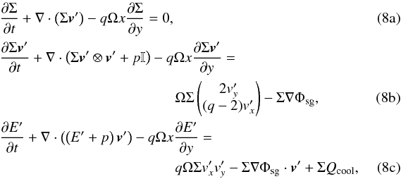 with the reduced energy density
  (9)The Fargo scheme (Masset 2000) has already been implemented in Fosite (Jung 2016) and can be enabled for v = v′ + w, where w is an arbitrary solenoidal velocity (Mignone et al. 2012).
2.2. Fictitious forces
The source terms for fictitious forces are implemented in two different ways according to the right hand sides of Eqs. (3b) and (3c), and Eqs. (8b) and (8c), respectively. The implementation differs depending on whether advection splitting is enabled or not.
2.3. Boundary conditions
We chose periodic boundary conditions in y-direction and sheared periodic boundary conditions in x-direction (Hawley et al. 1995). With  and Lx, Ly the size of the field in both directions we have
  (10)in the y-direction and
  (11)in the x-direction. If necessary, the data is linearly interpolated between adjacent cells (Hawley et al. 1995).
2.4. Self-gravity
We have considered a razor thin disk, which means that δ(z) in Eq. (4) is the δ-distribution, and solved this equation via common practice FFT routines2 similar to those in Gammie (2001). We shifted the surface density field to the next periodic point, transformed the result and calculated components of the potential via 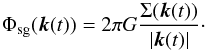 (12)Again transforming and shifting back gives us the solution for Φsg(x,y). The gravitational acceleration is obtained computing second order finite differences. We thereby also cut of all wavenumbers
  (Gammie 2001). Young & Clarke (2015) argue that this mimics the effect of a gravitational softening with length scale ~ 0.3H, where H is the scale height of the disk.
2.5. Viscosity
In order to measure the viscous stresses in a disk, the α prescription can be used (Shakura & Sunyaev 1973). Taking into account the cooling function in Eq. (5), an analytical expression for the dimensionless parameter α can be found (Gammie 2001):  (13)Simultaneously the α-parameter can be calculated from the simulations assuming a Jacobi-like integral (Gammie 2001), by splitting the stress-tensor Txy into a hydrodynamical part
  (14)with the residual velocities
  ,
,  and a gravitational part
  (15)Together these yield
  (16)Thus we can compare the numerical solution Eq. (16) with the analytical prediction in Eq. (13).
2.6. Numerical viscsosity
In order to resolve shocks, numerical schemes need to introduce non-linear terms. In SPH or finite difference schemes this is, for example, achieved by artificial viscosity. Fosite is based on finite volume methods which introduce limiters in order to handle the shock regions appropriately. Otherwise artificial numerical oscillations will occur in the vicinity of discontinuities. According to Godunov’s theorem (Godunov 1959) this is a fundamental limitation of linear difference schemes with higher than first order spatial accuracy. Essentially, the limiter is switching to first-order accuracy in the shock regions. In smooth regions an ideal limiter should not affect the numerical scheme. In the real world, however, any limiter effects the solutions even though the slopes are moderate. Slope-limiters, such as those in our case, are applied to the slopes of the physical quantities itself whereas flux-limiters, which were used in Paardekooper (2012), are applied to the fluxes. With a slope Δ, we introduced  (17)where φ(s) is the limiter which depends on the ratio of neighboring slopes s.
Within this text, we use two different limiters, VANLEER (van Leer 1974) and SUPERBEE (Roe & Baines 1982). VANLEER tends to lead to more numerical dissipation and resolves shocks less well than SUPERBEE. SUPERBEE, however, can oversteepen the slopes in shallow regions. A more thorough discussion on this issue can be found in Toro (2009), which gives an overview of some limiters applied to linear advection. This conforms to the guidelines of Hirsch (2007, Chap. 8.3.4), who additionally states that “limiters with continuous slopes generally favor convergence”. Whereas VANLEER has a continuous slope, limiters such as SUPERBEE or MINMOD (Roe 1986) show discontinuities in their slopes. The VANLEER limiter is described by  (18)and SUPERBEE by
  (19)
(19)
3. Tests and verification
We tested our code with epicyclic motion (Stone & Gardiner 2010; Paardekooper 2012) and linear theory (Gammie 2001; Paardekooper 2012). Thereby the linear theory test is being used extensively in order to obtain insights into the deviations between linear and non-linear simulations.
3.1. Epicyclic motion
The epicyclic motion test is adapted from Paardekooper (2012). We used exactly the same initial conditions with a resolution of Nx = Ny = 128, a field size of Lx = Ly = 1, an initial velocity perturbation vx,0 = 0.1cs and vy,0 = 0, with a speed of sound cs = 0.01. Then, we have oscillating solutions in the absence of any gradients  which holds for the Keplerian case.
Stone & Gardiner (2010) stress that the epicyclic energy  (22)should be conserved, which is achieved by a symmetric time integrator. Since Fosite is a purely explicit solver, we cannot conserve the epicyclic energy to round-off error. However, with the Dormand-Prince method (Dormand & Prince 1980), we ran the test over 1000 Ω-1 and get a relative error of order 10-5 for Eepi. Additionally Dormand-Prince is of fifth order accuracy, compared to the Crank-Nicholson method, which is symmetric but only of second order. In Fig. 1 the velocity evolution vx is shown over the first 1000 Ω-1.
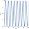 |
Fig. 1 Velocity perturbation for the epicyclic motion test over 100 Ω-1. There is no decline or increase of the amplitude. |
3.2. Linear theory
In order to test especially the gravitational solver (but also the boundaries and the fictitious forces) the equations of motion are linearized in Σ = Σ0 + δΣexp(ik(t)·x) (similarly for other variables) and the evolution of the amplitude of a small density wave is examined. For the isothermal case this is derived in Gammie (1996). Without magnetic fields and viscosity an ordinary differential equation 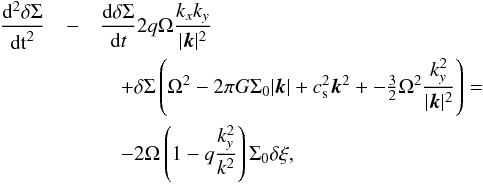 (23)is the result, where
  (24)is the initial perturbation in the vorticity ξ. See also Paardekooper (2012) for a thorough derivation. In Gammie (2001) the test is done including the energy equation, however we stay with the isothermal version to be comparable with Paardekooper (2012).
Similar to Paardekooper (2012) we used Eq. (23) with an initial perturbation of δΣ =5 × 10⁻⁴ Σ0 and Σ0 = 1. The wavenumbers are kx,0 = −2(2π) and ky,0 = 2π.
 |
Fig. 2 Density amplitude for the linear theory test with the VANLEER limiter. With increasing resolution, the numerical solution converges to the linear theory. |
In Fig. 2 we show convergence for the isothermal case with the VANLEER limiter. Typically, the first maximum is approximated well with all resolutions and limiters. At later stages the numerical viscosity plays a larger role with decreasing resolutions.
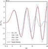 |
Fig. 3 Density amplitude for the linear theory test with the SUPERBEE limiter. No clear convergence, but rather an overestimation of the density amplitude is the case. |
Figure 3 shows the same setup, but using the SUPERBEE limiter. There, we do not see convergence, but an overestimation of the analytical theory at higher resolution. The error is largest for a resolution of N = 128 and then declines for higher resolutions. For N = 64 however, the behavior is similar to the one in Fig. 2. Thus it seems that we have two opposing effects, one has a declining, viscous nature, which one should expect, since numerical dissipation usually declines with increasing resolutions. The other varies strongly with the limiting function and it is only present or noticeable, if numerical dissipation is low enough, but leads to an excess in the density amplitude.
Since we expect that methods introduced to resolve shocks only add dissipation to the system, we would assume a lower amplitude over time. However, our test case inhibits no shocks, but shallow gradients. We therefore have strong indications that oversteepening caused by the SUPERBEE limiter is the reason for this effect (see e.g. Leveque 2002; Hirsch 2007, Chap. 6; Chap. 8).
Oversteepening is always present at shallow regions but comes only into effect when resolution is high enough, because the inherent discretization error of the numerical scheme which leads to numerical dissipation decreases. Shallow, shock free regions are the expected environment in which clumps form. To substantiate our thesis, we look more closely at our calculation with gravity from Fig. 2 (VANLEER) and Fig. 3 (SUPERBEE) at a resolution of N = 64. In Fig. 4
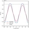 |
Fig. 4 Cut through the density field along the x-axis at position y = 0 and at time t = 520 Ω-1. The plateau of the SUPERBEE simulation is a clear indicator for oversteepening. The resolution is N = 64. |
a cut through the backshifted density field (by  ) along the x-axis at y = 0 and time t = 520Ω-1 is shown. This is shortly after the first transition through δΣ = 0. Comparing the solutions, we see firstly that the SUPERBEE simulation is overestimating the theoretical prediction, but this is mainly because the numerical solution is forerunning the analytical one at low resolutions (see Fig. 3). Secondly and most importantly the wave shows a clear plateau at the top of the waves. This is the common behavior and a clear indicator3 for an oversteepened function, which leads to considerable, non-physical deviations from the analytical solution.
We want to highlight under which circumstances the problem occurs in order to make predictions for a non-linear run. Therefore in Fig. 5
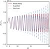 |
Fig. 5 Linear theory test at a resolution of 5122. The future behavior strongly depends on the limiting function and is qualitatively different. |
the test is shown twice as long for the highest resolution of 512 × 512 with different limiters. Over these timescales it can be observed that the error amplifies increasingly and even if the first 10 Ω-1 seem to be converged, at later stages the numerical solution diverges. Without the gravitational module in Fig. 6
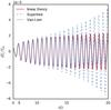 |
Fig. 6 Linear theory test without gravity at a resolution of 5122. The effect does not dependent on the self-gravitation but is purely numerical. |
the behavior remains the same, so gravitational forces are not the cause, but scale up initial errors.
We also tested the influence of a different time integrator (strong-stability-preserving Runge-Kutta method of same order, Macdonald 2003), a different Riemann solver (HLLC, Toro et al. 1994; Jung et al. 2015), with and without the advection splitting. We also carried out calculations with the energy equation. There are minor differences for different values of γ, but in all tests we performed, the limiting function plays the dominant role for the diverging nature of the test. We cannot exclude the possibility that the effect does not appear for the VANLEER limiter at higher resolutions and over longer timescales. Lastly, we also crosschecked the simulations with additional limiters, namely MINMOD (Roe 1986) and OSPRE (Waterson & Deconinck 1995), which also show convergence up to the resolution of N = 512 (very slowly for MINMOD, however).
There is an important difference to mention between our code and for example the one used by Paardekooper (2012). Our code limits the slopes in order to achieve a TVD-system (Illenseer & Duschl 2009) whereas Paardekooper (2012) uses flux limiting functions for the same purpose. Comparing simulations of linear advection, it seems that slope-limiters are more prone to oversteepening than flux-limiters (see Toro 2009, Chap. 13.10). However, the effect exists in both cases.
4. Non-linear results
The non-linear results with the VANLEER and SUPERBEE limiting functions are tested and the fragmentation boundary is investigated. If they both only add dissipation to the system, they should converge at high enough resolutions to the same macroscopic behavior, since the artificial heating added to the system should be low enough to exclude this as the major driver of non-convergence, as, for instance, Meru & Bate (2012) stated.
4.1. Standard run
Similar to Gammie (2001) we set L = 320 GΣ/Ω2 ~ 50 H with a resolution of N = 1024 and β = 2 or β = 10, respectively, and in order to be comparable we also used γ = 2.0. Up to 100 Ω-1, we can reproduce previous results with fragmentation for β = 2 and the gravito-turbulent state for β = 10.
For the following calculations, we used an initial β = 20 until t =50 Ω-1 and afterwards decrease β for the next 50 Ω-1 linearly to the desired value in order to avoid numerical problems from initializations (Paardekooper et al. 2011).
With the SUPERBEE limiter and β = 10 fragmentation occurs at t ≃ 300 Ω-1. We also can see the stochastic nature in this case. Therefore we ran the simulation with β = 15 twice until t = 1100 Ω-1, one simulation shows fragmentation, the other not. However, there is a difference to Paardekooper (2012): over the whole simulation time, fragmentation occurs most probably up to β ≲ 12. At the same time, with VANLEER limiter we see no fragmentation at all for β> 2 at a resolution of N = 1024.
4.2. The non-fragmenting case
We compare the non-linear outcome for both limiters and a large value of β, where the gravito-turbulent state is present throughout the simulation time. In Figs. 7 and 8 the macroscopic behavior can be seen at the end of the run with t = 1100 Ω-1, for the VANLEER and SUPERBEE limiter, respectively.
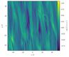 |
Fig. 7 Standard run for VANLEER limiter at the end of the Simulation at t = 1100 Ω-1. |
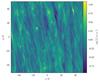 |
Fig. 8 Standard run for SUPERBEE limiter at the end of the Simulation at t = 1100 Ω-1. |
The simulation with SUPERBEE inhibits more structure and details. It shows small density enhancements, which did not lead to full fragmentation. These features are absent in the simulation with VANLEER limiter. Instead the gas is dominated by shocks running through the shearingsheet. Comparing our results with those of Gammie (2001, Fig. 4) and Baehr & Klahr (2015, Fig. 1 left), (with different cooling function) look much more like Fig. 7 at least qualitatively, whereas Fig. 8 can be associated with results presented in Paardekooper (2012, Fig. 6 top).
In Fig. 9 we show the maximum density Σmax together with the measured value of α. The simulation with the SUPERBEE limiter has generally a larger value for Σmax and a larger amplitude of variations in Σ. If β were smaller these excesses may lead to fragmentation. At the same time, α yields similar values, with slightly better results with SUPERBEE limiter. The VANLEER limiter shows a larger variance around a value slightly above the theoretical value of α = 0.011 calculated by Eq. (13). This is probably the case, because the VANLEER limiter is more dissipative, leading to additional heating. It can, however, also be seen that this value is not very large and shows that numerical heating has a minor, but not fully neglectable impact on the simulations.
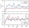 |
Fig. 9 The maximum surface density Σmax and the viscosity α for two different limiters and β = 20. The horizontal line is the theoretical value for α = 0.011. |
In Fig. 10 we see an overview of the fragmenting behavior. It shows fragmentation for β < 3 throughout. For a resolution of N = 512 both limiters have their fragmentation boundary directly at that value, very similar to Gammie (2001). At a larger resolution of N = 1024 this behavior changes dramatically. The VANLEER limiter has its boundary value still at the same value for β wheres the SUPERBEE limiter leads to fragmentation for at least up to β = 12. At N = 2048SUPERBEE behaves very similar. For the VANLEER limiter the largest value with which we see fragmentation is β = 5 at N = 2048. It should be mentioned that we do not get the slow way of fragmentation in that case, but local collapse directly at t = 100 Ω-1, where the final value of β is reached. Interestingly, Paardekooper (2012) obtains the same maximum result in βcrit for MINMOD, which generally is more dissipative. However, we cannot see any stochastic fragmentation for VANLEER limiter. It may still exists but then in a much tighter region around βcrit ~ 3−5. Generally the simulations at a resolution of N = 2048 where not performed over the whole 1100 Ω-1 but only up to 300 Ω-1, which is most probably the reason that we do not get fragmentation for β = 12 and the SUPERBEE limiter.
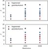 |
Fig. 10 Fragmentation plot for VANLEER limiter (top) and SUPERBEE limiter (bottom). The simulations where done for the resolution of 2048 only up to 300 Ω-1, compared to the other runs until 1100 Ω-1. This is the reason why there is only fragmentation up to β = 10 for the SUPERBEE limiter. |
In order to check our results coherently in comparison to other studies we also made simulations with MINMOD limiter and with γ = 1.6 ourself. MINMOD shows also fragmentation for β < 3 at a resolution of N = 1024 and no fragmentation for larger values. When choosing the smaller value for γ we also see fragmentation for VANLEER limiter and β = 5 at N = 1024. This is consistent with Rice et al. (2005), who state that lower a γ leads to larger critical βcrit.
5. Discussion
We have shown that the choice of the most appropriate limiting function is crucial to the non-linear outcome of the simulations and cannot be seen simply as a numerical helper adding more or less dissipation to the system. We have shown this for the special case of Goduvov type schemes which make use of slope limiters in order to achieve total-variation-diminishing.
Rice et al. (2014) showed that the cooling function needs to be adjusted in SPH simulations in order to converge. Young & Clarke (2015) however state that the gravitational smoothing leads to very different results in 2D simulations. Both publications thereby change physical quantities on small scales that are crucial for the fragmentation itself. Gravitational instabilities inherently depend on the cooling function and of course also on the gravitation itself. Thus, changing these quantities will always change the fragmentation behavior and could suppress any other physical or numerical effect on these scales. Still, we cannot exclude that these effects are the cause of fragmentation. Young & Clarke (2015) argue that smoothed 2D simulations cannot resolve the quasi-static collapse within their description. In other contexts, however, such as stochastic fragmentation, this poses no problem as 2D calculations by Young & Clarke (2016) demonstrate. The question of how strongly this effect evolves in three dimensions and together with gravity is an open one.
Additionally, we showed that oversteepening is also present without gravity and generally it is not affected by the number of dimensions, because of its pure numerical nature. The discussed numerical effect is dependent on neither gravitation, nor on the cooling function. We can also exclude that fragmentation for larger β ~ 10 is connected to numerical heating, since our results yield reasonable values for α. It takes place in exactly the region where clumps form and the error occurs on timescales which are comparable to the orbital timescales. It can also be backtracked to a well known effect called oversteepening and is testable with the linear theory test, at least in shearingsheet simulations. SPH codes introduce artificial stresses, which are always present, not only in shock regions, and some of them are especially introduced in order to avoid numerical fragmentation, because of, for instance, the testile instability (Monaghan 2000). This is why it cannot be excluded that SPH simulations also suffer from similar effects leading to an enhancement of density fluctuations which are in smooth regions scaled up by gravity.
This leads to an attractive property of oversteepening, as it may very well explain, why codes converge to different results or do not converge when β > 3. The artificial viscosities or limiters, which are introduced in order to resolve shocks well, are handled completely differently by different kinds of codes and probably also handle smooth gradients completely different.
Here, we have shown that the effect exists for Godunov-type schemes. This is, for example, also the case in Paardekooper (2012). In that case, the limiting functions are applied to other physical quantities (fluxes instead of slopes), which may change but not remove the effect. Our simulations run in concordance with the estimated behavior, because the effect tends to be stronger for slope limiters in the literature (Hirsch 2007), which we also see for our fragmentation behavior compared to Paardekooper (2012), both in the linear theory test and in the non-linear outcome.
With the SUPERBEE limiter we can also see stochastic fragmentation similar to Paardekooper (2012). Running at a resolution N = 1024 with β = 15 over tsim = 1100 Ω-1 twice, we observe fragmentation in one case only, but we did not investigate this issue in greater detail. With the other choice of the limiting function, we were not able to reproduce the stochastic features from Paardekooper (2012). They may indeed exist, but then in a much lower range then previously expected (around βcrit ≲ 5). This is also consistent with the results of Paardekooper (2012) himself, since he got βcrit ≲ 5 for the very dissipative limiter MINMOD, where most probably no oversteepening is present. With the VANLEER limiter, which is less dissipative, but also does not show oversteepening within the test, we get the same critical value for βcrit. Furthermore, independent SPH simulations by Young & Clarke (2016) show that the effect is not as strong as expected before.
Another important point to mention is that the statement of Young & Clarke (2015) that there is no dependency on γ in two-dimensional simulations is not coherent with our results. We can, for example, see fragmentation for β = 5 and the VANLEER limiter, when choosing γ = 1.6 and a resolution of N = 1024. This is in concurrency with the results of Rice et al. (2005), where it was stated that smaller γ lead to larger critical βcrit. Additionally, heat capacity ratios are often compared between two and three dimensions equivalently and although they might behave similarly, they are not the same (Gammie 2001).
6. Conclusions
In this paper, we investigated the impact of the limiting function on the fragmentation boundary in self-gravitating shearing-sheet simulations. By comparing the numerical outcome with linear theory, we showed that there is strong evidence that a unfortunate choice of the limiter can lead to an overestimation in the surface density in regions with shallow density gradients, which makes fragmentation easier for larger β. We accomplish this by using two-dimensional shearingsheet simulations and looking at deviations from to analytical results for linear theory. The behavior can be ascribed to a well known numerical effect called oversteepening, which occurs in regions with shallow density gradients. It is only observable if the resolution is high and the corresponding numerical diffusion low enough. Additionally, we can exclude gravity as the driving force of the effect, but it scales the small initial errors up. For the limiting functions where oversteepening sets in place in the test, we see very strong differences in the non-linear outcome. In these calculations we need much smaller critical βcrit, because of abundant density excesses in the field. We also cannot reproduce stochastic fragmentation with a well chosen limiter, however this might take place in a much smaller range for values of β.
We have used the following libraries: FFTW (Frigo & Johnson 2012) on scalar, fft (from MathKeisan package, see www.mathkeisan.com) on NEC-SX systems.
Together with steeper gradients, but the analytical solution gives us only the Fourier-component.
Acknowledgments
We thank an anonymous referee for very helpful comments on an earlier version of this paper.
References
- Baehr, H., & Klahr, H. 2015, ApJ, 814, 155 [Google Scholar]
- Boss, A. P. 1998, Nature, 393, 141 [NASA ADS] [CrossRef] [Google Scholar]
- Cossins, P., Lodato, G., & Clarke, C. J. 2009, MNRAS, 393, 1157 [Google Scholar]
- Dormand, J. R., & Prince, P. J. 1980, J. Comput. Appl. Math., 6, 19 [CrossRef] [MathSciNet] [Google Scholar]
- Frigo, M., & Johnson, S. G. 2012, Astrophys. Source Code Lib., [ascl:1201.015] [Google Scholar]
- Gammie, C. F. 1996, ApJ, 462, 725 [NASA ADS] [CrossRef] [Google Scholar]
- Gammie, C. F. 2001, ApJ, 553, 174 [NASA ADS] [CrossRef] [Google Scholar]
- Godunov, S. K. 1959, Matematicheskii Sbornik, 89, 271 [Google Scholar]
- Goldreich, P., & Lynden-Bell, D. 1965, MNRAS, 130, 125 [NASA ADS] [CrossRef] [Google Scholar]
- Hawley, J. F., Gammie, C. F., & Balbus, S. A. 1995, ApJ, 440, 742 [NASA ADS] [CrossRef] [Google Scholar]
- Hirsch, C. 2007, Numerical Computation of Internal and External Flows: Introduction to the Fundamentals of Cfd, Vol. 1, The Fundamentals of Computational Fluid Dynamics, 2nd edn. (Oxford, Burlington: Elsevier Ltd) [Google Scholar]
- Hopkins, P. F., & Christiansen, J. L. 2013, ApJ, 776, 48 [NASA ADS] [CrossRef] [Google Scholar]
- Illenseer, T. F., & Duschl, W. J. 2009, Comput. Phys. Commun., 180, 2283 [NASA ADS] [CrossRef] [Google Scholar]
- Jung, M. 2016, Ph.D. Thesis, Christian-Albrechts Universität Kiel [Google Scholar]
- Jung, M., Illenseer, T. F., & Duschl, W. J. 2015, Arxiv e-prints [arXiv:1505.06974] [Google Scholar]
- Kratter, K., & Lodato, G. 2016, ARA&A, 54, 271 [NASA ADS] [CrossRef] [Google Scholar]
- Kurganov, A., & Tadmor, E. 2000, J. Comput. Phys., 160, 241 [Google Scholar]
- Leveque, R. J. 2002, Finite Volume Methods for Hyperbolic Problems (Cambridge, New York: Cambridge University Press) [Google Scholar]
- Levin, Y., & Beloborodov, A. M. 2003, ApJ, 590, L33 [NASA ADS] [CrossRef] [Google Scholar]
- Lin, M.-K., & Kratter, K. M. 2016, ApJ, 824, 91 [NASA ADS] [CrossRef] [Google Scholar]
- Lodato, G., & Clarke, C. J. 2011, MNRAS, 413, 2735 [NASA ADS] [CrossRef] [Google Scholar]
- Macdonald, C. B. 2003, Master Thesis, Simon Fraser University [Google Scholar]
- Masset, F. 2000, A&AS, 141, 9 [Google Scholar]
- Meru, F., & Bate, M. R. 2011, MNRAS, 411, L1 [NASA ADS] [CrossRef] [Google Scholar]
- Meru, F., & Bate, M. R. 2012, MNRAS, 427, 2022 [NASA ADS] [CrossRef] [Google Scholar]
- Mignone, A., Flock, M., Stute, M., Kolb, S. M., & Muscianisi, G. 2012, A&A, 545, A152 [NASA ADS] [CrossRef] [EDP Sciences] [Google Scholar]
- Monaghan, J. J. 2000, J. Comput. Phys., 159, 290 [NASA ADS] [CrossRef] [Google Scholar]
- Müller, T. W. A., Kley, W., & Meru, F. 2012, A&A, 541, A123 [NASA ADS] [CrossRef] [EDP Sciences] [Google Scholar]
- Paardekooper, S.-J. 2012, MNRAS, 421, 3286 [NASA ADS] [CrossRef] [Google Scholar]
- Paardekooper, S.-J., Baruteau, C., & Meru, F. 2011, MNRAS, 416, L65 [NASA ADS] [CrossRef] [Google Scholar]
- Paczynski, B. 1978, Acta Astron., 28, 91 [Google Scholar]
- Rice, K. 2016, PASA, 33, e012 [Google Scholar]
- Rice, W. K. M., Lodato, G., & Armitage, P. J. 2005, MNRAS, 364, L56 [NASA ADS] [CrossRef] [Google Scholar]
- Rice, W. K. M., Forgan, D. H., & Armitage, P. J. 2012, MNRAS, 420, 1640 [NASA ADS] [CrossRef] [Google Scholar]
- Rice, W. K. M., Paardekooper, S.-J., Forgan, D. H., & Armitage, P. J. 2014, MNRAS, 438, 1593 [NASA ADS] [CrossRef] [Google Scholar]
- Roe, P. L. 1986, Ann. Rev. Fluid Mech., 18, 337 [NASA ADS] [CrossRef] [Google Scholar]
- Roe, P. L., & Baines, M. J. 1982, in Conf. Numerical Methods in Fluids Mechanics, Proc., 281 [Google Scholar]
- Shakura, N. I., & Sunyaev, R. A. 1973, A&A, 24, 337 [NASA ADS] [Google Scholar]
- Stone, J. M., & Gardiner, T. A. 2010, ApJS, 189, 142 [NASA ADS] [CrossRef] [Google Scholar]
- Toomre, A. 1964, ApJ, 139, 1217 [NASA ADS] [CrossRef] [Google Scholar]
- Toro, E. F. 2009, Riemann Solvers and Numerical Methods for Fluid Dynamics: A Practical Introduction, 3rd edn. (Dordrecht, New York: Springer) [Google Scholar]
- Toro, E. F., Spruce, M., & Speares, W. 1994, Shock Waves, 4, 25 [NASA ADS] [CrossRef] [EDP Sciences] [Google Scholar]
- van Leer, B. 1974, J. Comput. Phys., 14, 361 [NASA ADS] [CrossRef] [Google Scholar]
- Waterson, N. P., & Deconinck, H. 1995, Numerical Methods in Laminar and Turbulent Flow, 9, 203 [Google Scholar]
- Young, M. D., & Clarke, C. J. 2015, MNRAS, 451, 3987 [NASA ADS] [CrossRef] [Google Scholar]
- Young, M. D., & Clarke, C. J. 2016, MNRAS, 455, 1438 [NASA ADS] [CrossRef] [Google Scholar]
All Figures
|
Fig. 1 Velocity perturbation for the epicyclic motion test over 100 Ω-1. There is no decline or increase of the amplitude. |
| In the text | |
|
Fig. 2 Density amplitude for the linear theory test with the VANLEER limiter. With increasing resolution, the numerical solution converges to the linear theory. |
| In the text | |
|
Fig. 3 Density amplitude for the linear theory test with the SUPERBEE limiter. No clear convergence, but rather an overestimation of the density amplitude is the case. |
| In the text | |
|
Fig. 4 Cut through the density field along the x-axis at position y = 0 and at time t = 520 Ω-1. The plateau of the SUPERBEE simulation is a clear indicator for oversteepening. The resolution is N = 64. |
| In the text | |
|
Fig. 5 Linear theory test at a resolution of 5122. The future behavior strongly depends on the limiting function and is qualitatively different. |
| In the text | |
|
Fig. 6 Linear theory test without gravity at a resolution of 5122. The effect does not dependent on the self-gravitation but is purely numerical. |
| In the text | |
|
Fig. 7 Standard run for VANLEER limiter at the end of the Simulation at t = 1100 Ω-1. |
| In the text | |
|
Fig. 8 Standard run for SUPERBEE limiter at the end of the Simulation at t = 1100 Ω-1. |
| In the text | |
|
Fig. 9 The maximum surface density Σmax and the viscosity α for two different limiters and β = 20. The horizontal line is the theoretical value for α = 0.011. |
| In the text | |
|
Fig. 10 Fragmentation plot for VANLEER limiter (top) and SUPERBEE limiter (bottom). The simulations where done for the resolution of 2048 only up to 300 Ω-1, compared to the other runs until 1100 Ω-1. This is the reason why there is only fragmentation up to β = 10 for the SUPERBEE limiter. |
| In the text | |
Current usage metrics show cumulative count of Article Views (full-text article views including HTML views, PDF and ePub downloads, according to the available data) and Abstracts Views on Vision4Press platform.
Data correspond to usage on the plateform after 2015. The current usage metrics is available 48-96 hours after online publication and is updated daily on week days.
Initial download of the metrics may take a while.