Cosmological perturbations in the ΛCDM-like limit of a polytropic dark matter model

K. Kleidis; N. K. Spyrou

doi:10.1051/0004-6361/201630364

Home

All issues

Volume 606 (October 2017)

A&A, 606 (2017) A116

Full HTML

Free Access

Issue		A&A Volume 606, October 2017


Article Number		A116
Number of page(s)		13
Section		Cosmology (including clusters of galaxies)
DOI		https://doi.org/10.1051/0004-6361/201630364
Published online		23 October 2017

A&A 606, A116 (2017)

Cosmological perturbations in the ΛCDM-like limit of a polytropic dark matter model

K. Kleidis¹ and N. K. Spyrou²

¹ Department of Mechanical EngineeringTechnological Education Institute of Central Macedonia, 621.24 Serres, Greece
e-mail: kleidis@teiser.gr
² Department of Astronomy, Aristoteleion University of Thessaloniki, 541.24 Thessaloniki, Greece
e-mail: spyrou@auth.gr

Received: 27 December 2016
Accepted: 20 July 2017

Abstract

It has recently been proposed that both dark matter (DM) and dark energy (DE) can be treated as a single component when they are considered in the context of a polytropic DM fluid with thermodynamical content. Depending on only one free parameter, that is, the polytropic exponent, − 0.103 < Γ ≤ 0, this unified DM model reproduces the distance measurements performed with the aid of the supernovae Type Ia (SNe Ia) standard candles to high accuracy. It avoids the age problem and the coincidence problem, meaning that it allows interpreting not only when, but also why the Universe so recently transited from deceleration to acceleration. However, a critical problem still remains that the polytropic DM model is also required to solve, that is, it needs to demonstrate its compatibility with current observational data on structure formation. We begin to untie this knot here by discussing the evolution of cosmological perturbations in the ΛCDM-like (i.e., Γ = 0) limit of the polytropic DM model. The corresponding results are quite encouraging because this model reproduces every major effect known from conventional (i.e., pressureless cold dark matter – CDM) structure formation theory, such as the constancy of metric perturbations in the vicinity of recombination and the (late-time) Meszaros effect on their rest-mass density counterparts. The non-zero (polytropic) pressure, on the other hand, drives the evolution of small-scale velocity perturbations along the lines of the root-mean-square velocity law of conventional statistical physics. As a consequence, peculiar velocities in this model slightly increase instead of being redshifted away by cosmic expansion. This result might comprise a convenient probe of the polytropic DM model with Γ = 0. Even more importantly, however, upon consideration of scale-invariant metric perturbations, the spectrum of their rest-mass density counterparts exhibits an effective power-law dependence on the (physical) wavenumber, k_ph, of the form k_ph^{3+n_s^eff}, with the associated scalar spectral index, n_s^eff, being equal to n_s^eff = 0.970. This theoretical value reproduces the corresponding observational Planck result, that is, n_s^obs = 0.968 ± 0.006.

Key words: cosmological parameters / dark energy / dark matter / cosmology: theory

© ESO, 2017

1. Introduction

An extended list of observational data has recently suggested that in addition to the dark matter (DM) abundance and a (small) baryon contamination, the Universe also contains a uniformly distributed energy component with negative pressure. At relatively low values of cosmological redshift, z, this drives the cosmic expansion, causing the acceleration of the Universe (see, e.g., Olive et al. 2014). Reflecting our ignorance on its exact nature, this new component – which constitutes about two-thirds of the Universe mass-energy content – was termed dark energy – DE (Turner & White 1997; Perlmutter et al. 1999b).

The need for DE was first suggested by high-precision distance measurements, performed with the aid of supernovae Ia (SNe Ia) standard candles (Hamuy et al. 1996; Garnavich et al. 1998; Perlmutter et al. 1998, 1999a; Schmidt et al. 1998; Riess et al. 1998, 2001, 2004, 2007; Knop et al. 2003; Tonry et al. 2003; Barris et al. 2004; Krisciunas et al. 2005; Astier et al. 2006; Jha et al. 2006; Miknaitis et al. 2007; Wood-Vasey et al. 2007; Amanullah et al. 2008, 2010; Holtzman et al. 2008; Kowalski et al. 2008; Hicken et al. 2009a, 2009b; Kessler et al. 2009; Contreras et al. 2010; Guy et al. 2010; Suzuki et al. 2012). Today, observational data in favor of a distributed extra-energy component include evidence from galaxy clusters (Allen et al. 2004), the integrated Sachs-Wolfe (ISW) effect (Boughn & Crittenden 2004), baryon acoustic oscillations (BAOs; Eisenstein et al. 2005; Percival et al. 2010), weak gravitational lensing (WGL; Huterer 2002; Copeland et al. 2006), and the Lyman-α (LYA) forest (Seljak et al. 2006). A combination of these data with those from the Wilkinson microwave anisotropy probe (WMAP) survey (see, e.g., Komatsu et al. 2011; Bennett et al. 2013) has provided evidence for cosmic acceleration (and therefore for DE as well) at the 5σ confidence level.

Although the notion of DE can be attributed to a non-vanishing cosmological constant, Λ (see, e.g., Riess et al. 1998; Perlmutter et al. 1999a), this choice fails to explain the magnitude of Λ itself, since the corresponding theoretical predictions are 10¹²³ times larger than what is observed (cf. Sahni & Starobinsky 2000; Padmanabhan 2003). As a consequence, many other physically motivated models have been published, including quintessence (Caldwell et al. 1998), k-essence (Armendariz-Picon et al. 2001), phantom cosmology (Caldwell 2002), and tachyonic matter (Padmanabhan 2002), involving (also) several braneworld scenarios, such as DGP-gravity (Dvali et al. 2000) and the landscape scenario (Bousso & Polchinski 2000), as well as alternative-gravity theories, such as the scalar-tensor theories (Esposito-Farese & Polarski 2001), f(R)-gravity (Capozziello et al. 2003), and modified gravity (Nojiri & Odintsov 2007), holographic gravity (Cohen et al. 1999; Li 2004; Pavón & Zimdahl 2005), Chaplygin gas (Kamenshchik et al. 2001; Bento et al. 2002; Bean & Doré 2003; Sen & Scherrer 2005), Cardassian cosmology (Freese & Lewis 2002; Gondolo & Freese 2003; Wang et al. 2003), theories of compactified internal dimensions (Mongan 2001; Deffayet et al. 2002; Perivolaropoulos 2003; Sami et al. 2004), mass-varying neutrinos (Fardon et al. 2004; Peccei 2005), and so on (for a detailed review on the various DE models see, e.g., Caldwell & Kamionkowski 2009; Miao et al. 2011).

Of these models, the so-called unified DM models (see, e.g., Zimdahl et al. 2001; Bilić et al. 2002; Balakin et al. 2003; Gondolo & Freese 2003; Makler et al. 2003; Scherrer 2004; Ren & Meng 2006; Meng et al. 2007; Lima et al. 2008, 2010, 2012; Basilakos & Plionis 2009, 2010; Dutta & Scherrer 2010; Xu et al. 2012) have attracted much attention. In these models, both DM and DE can be described in terms of a single component, namely, the self-interacting DM (see, e.g., Spergel & Steinhardt 2000; Arkani-Hamed et al. 2009; Cirelli et al. 2009; Cohen & Zurek 2010; Van den Aarssen et al. 2012). This possibility is strongly suggested by observational data from the WMAP survey (Hooper et al. 2007), which are further reenforced by recent results from the high-energy particle detector PAMELA (Adriani et al. 2009, 2010), the Alpha Magnetic Spectrometer (AMS) on the International Space Station (Aguilar et al. 2016), and the Fermi Large Area Telescope (LAT) survey (Albert et al. 2017).

In this context, Kleidis & Spyrou (2015) recently proposed that the self-interacting DM could (at least phenomenologically) convey to the Universe matter content some sort of fluid-like properties, and consequently lead to a conventional approach to the DE concept. If the DM constituents were to collide with each other frequently enough, thus enabling their (kinetic) energy to be redistributed, a uniform extra-energy component might be present in the Universe, given by the energy of the internal motions of a thermodynamically involved DM fluid. The thermodynamical processes that could lead to a description that would be compatible with the observed characteristics of the accelerating Universe would be polytropic in type.

Polytropic processes in a DM fluid have been most successfully used in modeling dark galactic haloes, which significantly improved the velocity dispersion profiles of galaxies (Bharadwaj & Kar 2003; Nunez et al. 2006; Zavala et al. 2006; Böhmer & Harko 2007; Saxton & Wu 2008; Su & Chen 2009; Saxton & Ferreras 2010; Saxton et al. 2016). On a cosmological level, polytropic (DM) models were first encountered as natural candidates for Cardassian cosmologies (see, e.g., Freese & Lewis 2002; Gondolo & Freese 2003; Wang et al. 2003; Freese 2005), and they have been widely used as phenomenological models of an additional self-contained DE cosmological fluid (see, e.g., Nojiri et al. 2005; Stefancić 2005; Mukhopadhyay et al. 2008; Karami et al. 2009; Karami & Abdolmaleki 2010a,b, 2012; Malekjani et al. 2011; Chavanis 2012; 2014a,b; Karami & Khaledian 2012; Asadzadeh et al. 2014). More recently, polytropic characteristics were also attributed to an effective cosmic fluid obtained in the context of generalized Galileon cosmology (Koutsoumbas et al. 2017).

Our approach, however, is completely different, since it does not involve any additional DE at all. We instead simply examined the dynamical properties of a cosmological model driven by a gravitating (DM) fluid with thermodynamical content, the volume elements of which perform polytropic flows. In this case, the energy of this fluid’s internal motions is also taken into account as a source of the universal gravitational field, as it should. As we proved (see Kleidis & Spyrou 2015, 2016), this form of energy can compensate for the additional energy needed to compromise spatial flatness, namely, to justify that today, the total energy density parameter is exactly unity. The polytropic (DM) model we proposed depends on only one free parameter, the polytropic exponent, − 0.103 < Γ ≤ 0, and does not suffer from either the age problem or from the coincidence problem. At the same time, this model reproduces to high accuracy the distance measurements performed with the aid of the SNe Ia standard candles, without the need for any exotic DE or the cosmological constant. Finally, the polytropic DM model most naturally interprets not only when, but also why the Universe so recently transited from deceleration to acceleration, thus rising as a mighty contestant for a realistic (if conventional) DE model. However, a critical problem still remains that this model needs to solve. It needs to demonstrate its compatibility with current observational data concerning structure formation.

The theory of structure formation is based on gravitational instability and aims at describing how primordial fluctuations in matter grow into galaxies and cluster of galaxies through self-gravity. A perturbative approach can be used when the amplitudes of these fluctuations are small; hence, their growth can be solved to linear approximation. Cosmological perturbations over a homogeneous and isotropic background, as they historically developed (Lifshitz 1946; Lifshitz & Khalatnikov 1963; Hawking 1966; Sachs & Wolfe 1967; Weinberg 1972; Peebles 1980; Mukhanov et al. 1992; Padmanabhan 1993), are well suited to describe a curved background that is filled with ordinary matter, the stress-energy tensor of which can be described in terms of an equation of state. This theory has been most successfully used to study the growth of inhomogeneities in radiation, baryonic matter, and DM (see, e.g., Ma & Bertschinger 1995).

At this point, we should note that as far as structure formation is concerned, all forms of DM are not equivalent. Particles that are highly relativistic (such as neutrinos or other particles with masses lower than 100 eV/c²) have the property that free streaming erases perturbations out to very large scales (Bond et al. 1980). In this case, very large-scale structures form first and subsequently fragment to form galaxies later. Particles with this property are termed hot dark matter (HDM). On the other hand, CDM (i.e., particles with masses higher than 1 MeV/c²) has the opposite behavior: small-scale structures form first, aggregating to form larger structures later (Bond & Szalay 1983). It is now well known that pure HDM cosmologies cannot reproduce the observed large-scale structure of the Universe (see, e.g., Klypin et al. 1993), in contrast to the CDM cosmologies, which are considered to be pressureless, however. As a consequence, the evolution of cosmological perturbations in CDM models has been restricted to the Newtonian regime (see, e.g., Veeraraghavan & Stebbins 1990; Knobel 2012).

Nevertheless, in the polytropic DM approach, we do not neglect the pressure, p, with respect to the overall energy density, ε. This means that even well within the matter-dominated era, cosmological perturbations should be treated in a general-relativistic manner. To define the energy density perturbation, we need to choose a particular set of hypersurfaces in this context, meaning that we need to choose a gauge. The (so-called) Newtonian gauge (Mukhanov et al. 1992) is a particularly convenient choice to treat scalar perturbations because in this case, the scalar fields that describe the metric perturbations are identical (up to a minus sign) to the gauge-invariant variables introduced by Bardeen (1980). For this reason, we here adopt the Newtonian gauge.

This paper is organized as follows. In Sect. 2 we summarize the basic features of the polytropic DM model and its ΛCDM-like (Γ = 0) limit. In Sect. 3 we present the mathematical setup that leads to the system of differential equations that govern the evolution of small-scale fluctuations in a (dark-) matter-dominated Universe, perturbed over a spatially flat Friedmann-Robertson-Walker (FRW) model, the (zeroth-order) evolution of which is driven by a polytropic (DM) fluid with thermodynamical content. In Sect. 4 we restrict ourselves to the ΛCDM-like (i.e., Γ = 0) limit of this model. In this case, the perturbation equations decouple and can be solved analytically, to give the form of the generalized Newtonian potential, φ, as a function of the cosmological redshift, z. Accordingly, the rest-mass density contrast, δ, and the comoving counterpart, υ, of the peculiar velocity field, υ_pec, are also obtained as functions of z. A subsequent analysis of these results shows that our solution for { φ,δ } can reproduce every major effect previously known from conventional (i.e., pressureless CDM) cosmological perturbation theory. In particular, at 100 ≤ z ≤ 1090, the generalized Newtonian potential is | φ | ≈ const., justifying the current scientific perception that during the early matter-dominated era, the metric perturbations were (more or less) constant (see, e.g., Knobel). In matter perturbations, the corresponding small-scale modes (i.e., those lying well within the horizon) conform with the (so-called) Meszaros effect (Meszaros 1974). In contrast, modes of linear dimensions that are comparable to the horizon length are suppressed as ${(1 + z^{)}}^{-1}$ $\hbox{$\left ( 1 + z \right )^{-1}$}$ , which means that at relatively high values of z(100 ≤ z ≤ 1090), only the small-scale structures we see today were allowed to be formed. We expect that on the approach to the present epoch (i.e., at lower cosmological redshift values), these small-scale structures must have subsequently aggregated to form macrostructures, in compatibility with the CDM approach. On the other hand, because of the non-zero polytropic pressure, peculiar velocities are no longer redshifted away, as is predicted by conventional (i.e., pressureless) structure formation theory (see, e.g., Peacock 1999; Sparke & Ghallagher 2007). Instead, along the lines of the root-mean-square (rms) velocity law of statistical physics, υ increases in proportion to the square root of the Universe scale factor, R, although it still remains conveniently small (e.g., for z ≥ 100, υ ≤ 10^-3 ≪ 1). We explore in Sect. 5 the dimensionless power spectrum of rest-mass density perturbations in the ΛCDM-like (i.e., p = const. ≠ 0) limit of the unified DM model under consideration. Provided that the spectrum of metric perturbations is scale invariant, as implied by the cosmic microwave background (CMB) anisotropy measurements (see, e.g., Komatsu et al. 2009, 2011) and several other physical arguments (see, e.g., Padmanabhan 1993; Peacock 1999), its rest-mass density counterpart exhibits an effective power-law dependence on the (physical) wavenumber, k_ph, of the form $k_{ph}^{3 + n_{s}^{eff}}$ $\hbox{$k_{\rm ph}^{3+n_{\rm s}^{\rm eff}}$}$ , with the associated scalar spectral index, $n_{s}^{eff}$ $\hbox{$n_{\rm s}^{\rm eff}$}$ , being equal to $n_{s}^{eff} = 0.970$ $\hbox{$n_{\rm s}^{\rm eff} = 0.970$}$ . This value differs only slightly from the corresponding observational Planck result, which is 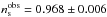$n_{s}^{obs} = 0.968 \pm 0.006$ $\hbox{$n_{\rm s}^{\rm obs} = 0.968 \pm 0.006$}$ (Planck Collaboration XIII 2016). To the best of our knowledge, this is the first time that a conventional model with practically no free parameters predicts a theoretical result so close to observation. Finally, we conclude in Sect. 6. In what follows, we consider c = 1 =ħ.

2. Polytropic (DM) semantics

Kleidis & Spyrou (2015) recently explored the properties and associated phenomenology of a (spatially flat) cosmological model in the context of a unified DM scenario. In this model, the fundamental units of the Universe matter-energy content are the volume elements of a collisional DM fluid performing polytropic flows. In this case, the (isotropic) pressure, p, of the cosmic fluid is related to its rest-mass density, ρ, through the barotropic equation of state (EoS), $p = p_{0} {(\frac{ρ}{ρ_{0}})}^{Γ},$ $\begin{equation} p = p_0 \left ( \frac{\rh}{\rh_0} \right )^{\Gm}, \end{equation}$ (1)where p₀ and ρ₀ are the associated present-time values and Γ is the polytropic exponent (in connection, see, e.g., Chandrasekhar 1939; Horedt 2004).

Along with all the other physical characteristics, the internal thermodynamic energy of the cosmic fluid also needs to be taken into account as a source of the universal gravitational field in this context. In other words, in a polytropic cosmological model the overall energy density, ε, of the Universe matter-energy content is no longer given solely by its rest-mass counterpart, ρ, but also includes an additional term, $\hbox{$\rh {\cal U}$}$ , which is associated with the energy of the cosmic fluid’s internal motions, $\hbox{${\cal U}$}$ , per unit of specific volume, $\frac{1}{ρ}$ $\hbox{$\frac{1}{\rh}$}$ (for a detailed analysis, see, e.g., Fock 1959). This form of energy may serve as the DE needed to compromise spatial flatness (cf. Eqs. (49)–(50) of Kleidis & Spyrou 2015), that is, to justify that today, the overall energy density parameter, Ω, is very close to unity (see, e.g., Komatsu 2009, 2011). This is much higher than the measured value of its rest-mass counterpart, Ω_M = 0.308 (Planck Collaboration XIII 2016).

In a perfectly fluid source, the combination of the continuity equation, $𝒯_{; ν}^{0 ν} = 0,$ $\begin{equation} {\cal T}^{0 \nu}_{; \nu} = 0, \end{equation}$ (2)where $\hbox{${\cal T}^{\mu \nu}$}$ is the energy-momentum tensor of the Universe matter-energy content (Greek indices, μ,ν = 0,1,2,3, refer to four-dimensional spacetime, and the semicolon denotes the covariant derivative), with the first law of thermodynamics in curved spacetime, 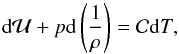$d𝒰 + p d (\frac{1}{ρ}) = 𝒞d T,$ $\begin{equation} {\rm d} {\cal U} + p{\rm d} \left ( \frac{1}{\rh} \right ) = {\cal C} {\rm d}T, \end{equation}$ (3)where T is the polytropic-DM temperature and $\hbox{${\cal C}$}$ is the associated specific heat, result in the decomposition of ε as 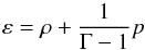$ε = ρ + \frac{1}{Γ - 1} p$ $\begin{equation} \varep = \rh + \frac{1}{\Gm - 1} p \end{equation}$ (4)(cf. Eq. (39) of Kleidis & Spyrou 2015), where we have also taken into account that in a closed thermodynamical system (e.g., any volume element of the fluid-like model so considered) the total number of particles is conserved; hence, 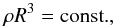$ρ R^{3} = const .,$ $\begin{equation} \rh R^3 = \textrm{const.}, \end{equation}$ (5)with R being the Universe scale factor. Accordingly, inserting Eq. (4) into the Friedmann equation, 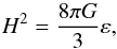$H^{2} = \frac{8 πG}{3} ε,$ $\begin{equation} H^2 = \frac{8 \pi G}{3} \varep, \end{equation}$ (6)where \begin{lxirformule}$H = \frac{\dot{R}}{R}$\end{lxirformule} is the Hubble parameter, G is Newton’s universal constant of gravitation, and the dot denotes differentiation with respect to cosmic time, t, we obtain ${(\frac{H}{H_{0}})}^{2} = Ω_{M} {(\frac{R_{0}}{R})}^{3} [1 + \frac{1}{Γ - 1} \frac{p_{0}}{ρ_{0}} {(\frac{R_{0}}{R})}^{3 (Γ - 1)}]$ $\begin{equation} \left ( \frac{H}{H_0} \right )^2 = \Om_{\rm M} \left ( \frac{R_0}{R} \right )^3 \left [ 1 + \frac{1}{\Gm - 1} \frac{p_0}{\rh_0} \left ( \frac{R_0}{R} \right )^{3 (\Gm - 1)} \right ] \end{equation}$ (7)(cf. Eq. (43) of Kleidis & Spyrou 2015), with H₀ and R₀ representing the present-time values of H and R, respectively. As a consequence, today, Eq. 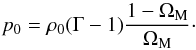(7) is reduced to $p_{0} = ρ_{0} (Γ - 1) \frac{1 - Ω_{M}}{Ω_{M}} \cdot$ $\begin{equation} p_0 = \rh_0 (\Gm - 1) \frac{1 - \Om_{\rm M}}{\Om_{\rm M}} \cdot \end{equation}$ (8)In view of Eq. (8), for Γ < 1, the pressure given by Eq. (1) becomes negative, and so does the quantity ε + 3p at cosmological redshifts, $z \equiv \frac{R_{0}}{R} - 1$ $\hbox{$z \equiv \frac{R_0}{R} - 1$}$ , lower than a transition value, z_tr (cf. Eqs. (107)–(108) of Kleidis & Spyrou 2015). In other words, for z ≤ z_tr, a cosmological model filled with polytropic DM fluid accelerates its expansion. Upon consideration of Eq. (8), the Friedmann equation (7) reads 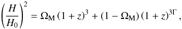${(\frac{H}{H_{0}})}^{2} = Ω_{M} {(1 + z^{)}}^{3} + (1 - Ω_{M}) {(1 + z^{)}}^{3 Γ},$ $\begin{equation} \left ( \frac{H}{H_0} \right )^2 = \Om_{\rm M} \left ( 1 + z \right )^3 + (1 - \Om_{\rm M}) \left ( 1 + z \right )^{3 \Gm}, \end{equation}$ (9)representing a (spatially flat) cosmological model filled with CDM and (dynamically evolving) DE (see, e.g., Linder & Jenkins 2003, Eq. (2); Amendola et al. 2013, Eq. (1.3.1)), the amount of which at the present epoch rises to 1 − Ω_M = 0.692 of the Universe matter-energy content (Planck Collaboration XIII 2016).

It is worth noting that for Γ = 0, the theoretically derived value for z_tr (cf. Eq. (72) of Kleidis & Spyrou 2015) reproduces the corresponding ΛCDM result (see, e.g., Capozziello et al. 2015, Eq. (20)). For Γ = 0, the polytropic cosmological model under consideration reproduces every main aspect of the widely used ΛCDM model (cf. Eq. (9), above), such as the Universe expansion law, R(t) ~ sinh^{2 / 3}t (see, e.g., Frieman et al. 2008), and the associated “age”, t₀ ≈ 13.80 billion years (cf. Kleidis & Spyrou 2015, Eqs. (64) and (66), respectively). For Ω_M = 0.308 (Planck Collaboration XIII 2016), it (furthermore) reproduces the present-time value, q₀, of the deceleration parameter, q, predicting q₀ = − 0.54, whereas current observational data suggest that $q_{0} = - 0.5 3_{-0.13}^{+ 0.17}$ $\hbox{$q_0 = - 0.53_{-0.13}^{+0.17}$}$ (see, e.g., Giostri et al. 2012), and the ΛCDM-oriented value of the CMB-shift parameter, in which case, the Γ = 0 limit of the polytropic DM model predicts ℛ = 1.7342 (cf. Kleidis & Spyrou 2015, Eq. (112)), whereas the nine-year WMAP survey (Bennett et al. 2013) suggests that ℛ = 1.7329 ± 0.0058 (68% CL). In view of all the above, the polytropic DM model with Γ = 0 is termed throughout the “ΛCDM-like limit of the polytropic DM model”.

In this limit, the polytropic DM model under consideration fully compromises the parameterization of the (so-called) total EoS parameter, $w_{tot} \equiv \frac{p}{ε},$ $\begin{equation} w_{\rm tot} \equiv \frac{p}{\varep}, \end{equation}$ (10)in terms of z. For Γ = 0, upon consideration of Eqs. (4), (5), and (8), Eq. (10) yields 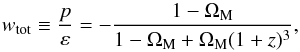$w_{tot} \equiv \frac{p}{ε} = - \frac{1 - Ω_{M}}{1 - Ω_{M} + Ω_{M} (1 + z)^{3}},$ $\begin{equation} w_{\rm tot} \equiv \frac{p}{\varep} = - \frac{1 - \Om_{\rm M}}{1 - \Om_{\rm M} + \Om_{\rm M} (1 + z)^3}, \end{equation}$ (11)the evolution of which is presented in Fig. 1 as a function of z. We observe that today, that is, for z = 0, w_tot = − (1 − Ω_M) = − 0.692, in complete agreement with the corresponding ΛCDM result, 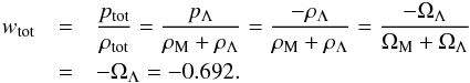$\begin{matrix} w_{tot} & = & \frac{p_{tot}}{ρ_{tot}} = \frac{p_{Λ}}{ρ_{M} + ρ_{Λ}} = \frac{- ρ_{Λ}}{ρ_{M} + ρ_{Λ}} = \frac{- Ω_{Λ}}{Ω_{M} + Ω_{Λ}} \\ = & - Ω_{Λ} = - 0.692. \end{matrix}$ $\begin{eqnarray} w_{\rm tot} &= &\frac{p_{\rm tot}}{\rh_{\rm tot}} = \frac{p_{\Lm}}{\rh_{\rm M} + \rh_{\Lm}} = \frac{- \rh_{\Lm}}{\rh_{\rm M} + \rh_{\Lm}} = \frac{- \Om_{\Lm}}{\Om_{\rm M} + \Om_{\Lm}} \nn \\ & = &- \Om_{\Lm} = - 0.692 . \end{eqnarray}$ (12)For Γ ≠ 0, several physical requirements in the context of the polytropic DM approach (such as a non-negative velocity-of-sound square, $c_{s}^{2}$ $\hbox{$c_{\rm s}^2$}$ , and the large-scale structure amendment for CDM) can lead to successive constraints on the polytropic exponent, the value of which for Ω_M = 0.308 settles down to the range − 0.103 < Γ ≤ 0. For each and every value of Γ in this range, the theoretically derived (in the framework of the polytropic DM model) expression of the luminosity distance, d_L(z), fits the Hubble diagram of the 580 standard candles (cf. Fig. 6 of Kleidis & Spyrou 2015) that constitute the Union 2.1 SNe Ia Compilation (Suzuki et al. 2012) to high accuracy. At the same time, this model avoids the so-called age problem (cf. Fig. 2 of Kleidis & Spyrou 2015) and significantly alleviates the coincidence problem (cf. Eqs. (106)–(108) of Kleidis & Spyrou 2015).

Fig. 1

Total EoS parameter, w_tot, as a function of the cosmological redshift, z, in the context of the ΛCDM-like (i.e., Γ = 0) limit of the polytropic DM model. We note that today, w_tot ≈ − 0.7, while for z ≥ 3, it remains very close to zero, as suggested by ΛCDM cosmology.

Nevertheless, we stress that it is still unclear what sort of microphysics would produce the postulated polytropic behavior; hence, our model is to be seen as an effective (phenomenological) approach of an elementary physics scenario that is yet to be discovered (see, e.g., Gondolo & Freese 2003; Arkani-Hamed et al. 2009; Van den Aarssen et al. 2012).

Finally, in a spatially flat cosmological model, the proper distance, D, is defined as D = R(t)r, where r is the comoving radial coordinate. The corresponding (proper) velocity is given by $v_{prop} \equiv \frac{d D}{d t} = HD + υ_{com} R = υ_{rec} + υ_{pec}$ $\hbox{$v_{\rm prop} \equiv \frac{{\rm d} D}{{\rm d} t} = H D + \ups_{\rm com} R = \ups_{\rm rec} + \ups_{\rm pec}$}$ , where υ_rec = HD is the recession velocity, driven by Hubble’s law, and υ_pec = υ_comR represents the so-called peculiar velocity field, with $υ_{com} = \frac{d r}{d t}$ $\hbox{$\ups_{\rm com} = \frac{{\rm d} r}{{\rm d} t}$}$ being its comoving counterpart (see, e.g., Peacock 1999, Eq. (15.17)). Accordingly, we would expect that in a cosmological model with thermodynamical content, peculiar velocities of the (non-relativistic) CDM units (e.g., the volume elements of the CDM fluid) conform with the rms-velocity law of statistical physics, that is, $⟨ υ_{pec} ⟩ = \sqrt{3 \frac{p}{ρ}}$ $\begin{equation} \langle \ups_{\rm pec} \rangle = \sqrt{3 \frac{p}{\rh}} \end{equation}$ (13)(see, e.g., Landau & Lifshitz 1969), where the brackets denote average values. On this basis, the comoving counterpart of the peculiar velocity field, υ ≡ ⟨ υ_com ⟩, obeys the relation $⟨ υ_{com} ⟩ = \frac{1}{R} \sqrt{3 \frac{p}{ρ}} \cdot$ $\begin{equation} \langle \ups_{\rm com} \rangle = \frac{1}{R} \sqrt{3 \frac{p}{\rh}}\cdot \end{equation}$ (14)Equation (13) (or, equivalently, Eq. (14)) is yet to be confirmed for the polytropic CDM approach to be self-contained (in connection, however, see Sect. 4, discussion on Fig. 5).

In view of all the above advantages and disadvantages, the polytropic CDM model under consideration can rise from the rank as a mighty contestant for a viable (if conventional) DE model. However, a critical problem remains that this model also needs to solve, that is, it needs to demonstrate its compatibility with current observational data of structure formation.

3. Perturbation equations in Fourier space

The Newtonian (longitudinal) gauge, particularly advocated by Mukhanov et al. (1992), has the advantage that the gauge-invariant quantities coincide with the corresponding physical quantities. Consequently, in a model where the overall energy density is due to an ideal fluid, it is reasonable to neglect any anisotropic stresses. In such a model, only one metric perturbation remains undetermined, namely, the generalized Newtonian potential (see, e.g., Knobel 2012). Accordingly, the cosmological spacetime metric of a (dark-) matter-dominated Universe perturbed over a spatially flat FRW model is written in the form $d s^{2} = R^{2} (η) [(1 - 2 φ) d η^{2} - (1 + 2 φ) δ_{ij} d x^{i} d x^{j}]$ $\begin{equation} {\rm d}s^2 = R^2 (\et) \left [ \left ( 1 - 2 \phi \right ) {\rm d} \et^2 - \left ( 1 + 2 \phi \right ) \dl_{ij} {\rm d}x^i {\rm d}x^j \right ] \end{equation}$ (15)(see, e.g., Ma & Bertschinger 1995), where R(η) is the scale factor in terms of conformal time, $η = {^{\int}}^{t} \frac{d t}{R (t)}$ $\hbox{$\et = \int^t \frac{{\rm d}t}{R(t)}$}$ , Latin indices (i,j = 1,2,3) refer to the three-dimensional spatial slices of the four-dimensional spacetime, δ_ij is the Kronecker symbol, and φ is the scalar gravitational potential. It is worth noting that in general, perturbations, δg_μν, over the metric tensor, g_μν, also contain contributions from vector and tensor fields, which exhibit no instabilities, however. In an expanding Universe, vector perturbations decay kinematically, whereas tensor perturbations lead to gravitational waves, which do not couple with energy density and pressure inhomogeneities (see, e.g., Bardeen 1980). The scalar perturbations alone can lead to growing inhomogeneities, which in turn have an important effect on the dynamics of matter (see, e.g., Kodama & Sasaki 1984).

The metric perturbation, φ, is a solution to the perturbed Einstein equations $δ 𝒢_{μν} = - 8 πGδ 𝒯_{μν},$ $\begin{equation} \dl {\cal G}_{\mu \nu} = - 8 \pi G \dl {\cal T}_{\mu \nu}, \end{equation}$ (16)where $\hbox{$\dl {\cal G}_{\mu \nu}$}$ are small-scale fluctuations of the homonymous tensor, $\hbox{${\cal G}_{\mu \nu}$}$ , and $\hbox{$\dl {\cal T}_{\mu \nu}$}$ is the energy-momentum tensor of the Universe matter-energy content perturbed over a perfect-fluid source $𝒯_{μν} = (ε + p) u_{μ} u_{ν} - g_{μν} p .$ $\begin{equation} {\cal T}_{\mu \nu} = (\varep + p) u_{\mu} u_{\nu} - g_{\mu \nu} p . \end{equation}$ (17)In Eq. (17), $u^{μ} = \frac{d x^{μ}}{d s} = (\frac{1}{R}, 0, 0, 0)$ $\begin{equation} u^{\mu} = \frac{{\rm d} x^{\mu}}{{\rm d}s} = \left ( \frac{1}{R}, 0, 0, 0 \right ) \end{equation}$ (18)is the (unperturbed) four-velocity of the fluid comoving with Universe expansion. Accordingly, deviations from Hubble flow, that is, peculiar fluctuations over u^μ, can be cast in the form $δ u^{μ} = \frac{1}{R} (0, υ^{1}, υ^{2}, υ^{3}),$ $\begin{equation} \dl u^{\mu} = \frac{1}{R} \left ( 0, \ups^1, \ups^2, \ups^3 \right ), \end{equation}$ (19)where υⁱ = dxⁱ/ dη are the comoving components of the slow (as compared to the Universe expansion rate) peculiar velocity of the fluid (in terms of conformal time). In this case, $δ u_{i} = g_{ij} \frac{1}{R} υ^{j} = - R^{2} δ_{ij} \frac{1}{R} υ^{j} + O_{2} ≃ - R υ_{i},$ $\begin{equation} \dl u_i = g_{ij} \frac{1}{R} \ups^j = - R^2 \dl_{ij} \frac{1}{R} \ups^j + O_2 \simeq - R \ups_i, \end{equation}$ (20)where the symbol O₂ denotes terms of second order in the (small) quantities υ, φ, and $\frac{δρ}{ρ}$ $\hbox{$\frac{\dl \rh}{\rh}$}$ , with δρ being the rest-mass density perturbation. As given by Eq. (20), δu_i is dimensionless, and the total four-velocity, U^μ = u^μ + δu^μ, satisfies the condition $U_{μ} U^{μ} = (u_{μ} + δ u_{μ}) (u^{μ} + δ u^{μ}) = 1 + O_{2}$ $\begin{equation} U_{\mu} U^{\mu} = \left ( u_{\mu} + \dl u_{\mu} \right ) \left ( u^{\mu} + \dl u^{\mu} \right ) = 1 + O_2 \: \end{equation}$ (21)to linear terms in υⁱ.

In this model, the evolution of cosmological perturbations (in Fourier space) is governed by two sets of differential equations (see, e.g., Kodama & Sasaki 1984; Veeraraghavan & Stebbins 1990; Mukhanov et al. 1992; Padmanabhan 1993; Ma & Bertschinger 1995; Mukhanov 2005; Knobel 2012, and references therein).

Field equations:

$\begin{matrix} - k^{2} φ - 3 ℋ (φ^{'} + ℋ φ) = 4 πG R^{2} δε, \\ φ^{'} + ℋ φ = 4 πG R^{2} (ε + p) \frac{υ}{k}, \\ φ^{′′} + 3 ℋ φ^{'} + (2 ℋ^{'} + ℋ^{2}) φ = 4 πG R^{2} δp . \end{matrix}$ $\begin{eqnarray} &&-k^2 \phi - 3 {\cal H} \left ( \phi^{\prime} + {\cal H} \phi \right ) = 4 \pi G R^2 \dl \varep, \\ &&\phi^{\prime} + {\cal H} \phi = 4 \pi G R^2 (\varep + p) \frac{\ups}{k}, \\ &&\phi^{\prime \prime} + 3 {\cal H} \phi^{\prime} + \left ( 2 {\cal H}^{\prime} + {\cal H}^2 \right ) \phi = 4 \pi G R^2 \dl p. \end{eqnarray}$

Equations of motion:

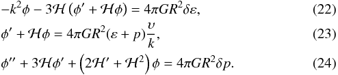
$\begin{matrix} (\partial_{η} + 3 ℋ^{)} δε + 3 ℋ δp = - (ε + p) (kυ - 3 φ^{'}), \\ (\partial_{η} + 4 ℋ^{)} [\frac{υ}{k} (ε + p)] = δp + (ε + p) φ . \end{matrix}$ $\begin{eqnarray} &&\left ( \partial_{\et} + 3 {\cal H} \right ) \dl \varep + 3 {\cal H} \dl p = - (\varep + p) \left (k \ups - 3 \phi^{\prime} \right ), \\ &&\left ( \partial_{\et} + 4 {\cal H} \right ) \left [ \frac{\ups}{k} (\varep + p) \right ] = \dl p + (\varep + p) \phi. \end{eqnarray}$ In Eqs. 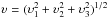(22)–(26), δε and δp are small-scale perturbations to the overall energy density and pressure, respectively, k is the comoving wavenumber of the pertubation modes, $υ = (υ_{1}^{2} + υ_{2}^{2} + υ_{3}^{2})^{1 / 2}$ $\hbox{$\ups = ( \ups_1^2 + \ups_2^2 + \ups_3^2 )^{1/2}$}$ is the comoving peculiar velocity of the mode denoted by k, and we have set $ℋ = \frac{R^{'}}{R}$ $\hbox{${\cal H} = \frac{R^{\prime}}{R}$}$ with the prime denoting differentiation with respect to η, ∂_η.

In an FRW model, the unperturbed quantities ℋ, ε and p are related by the Friedmann equations (in terms of conformal time) 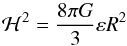$ℋ^{2} = \frac{8 πG}{3} εR 2$ $\begin{equation} {\cal H}^2 = \frac{8 \pi G}{3} \varep R^2 \end{equation}$ (27)and 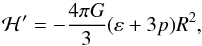$ℋ^{'} = - \frac{4 πG}{3} (ε + 3 p) R^{2},$ $\begin{equation} {\cal H}^{\prime} = - \frac{4 \pi G}{3} ( \varep + 3 p ) R^2, \end{equation}$ (28)along with the (unperturbed) conservation law given by Eq. (2), which reduces to 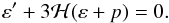$ε^{'} + 3 ℋ (ε + p) = 0.$ $\begin{equation} \varep^{\prime} + 3 {\cal H} ( \varep + p ) = 0. \end{equation}$ (29)The combination of Eq. (29) with the particle number conservation law, 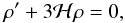$ρ^{'} + 3 ℋ ρ = 0,$ $\begin{equation} \rh^{\prime} + 3 {\cal H} \rh = 0, \end{equation}$ (30)yields $p^{'} + 3 Γℋ p = 0 \Rightarrow p R^{3 Γ} = const .,$ $\begin{equation} p^{\prime} + 3 \Gm {\cal H} p = 0 \Rightarrow p R^{3 \Gm} = \textrm{const.}, \end{equation}$ (31)verifying the fundamental polytropic relation pV^Γ = const., where V = R³ is the comoving volume element. Equation (31) suggests that in a cosmological model filled with polytropic (DM) fluid, the pressure is a slowly increasing (since − 0.103 ≤ Γ ≤ 0) function of R, hence, of η, or/and t, as well.

In view of Eq. (4), the perturbation quantities δε and δp are no longer independent, being related by 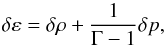$δε = δρ + \frac{1}{Γ - 1} δp,$ $\begin{equation} \dl \varep = \dl \rh + \frac{1}{\Gm - 1} \dl p, \end{equation}$ (32)where by virtue of Eq. (1), $\frac{δp}{p} = Γ \frac{δρ}{ρ},$ $\begin{equation} \frac{\dl p}{p} = \Gm \frac{\dl \rh}{\rh}, \end{equation}$ (33)and therefore, $δε = [1 + \frac{Γ}{Γ - 1} (\frac{p}{ρ})] δρ .$ $\begin{equation} \dl \varep = \left [ 1 + \frac{\Gm}{\Gm - 1} \left ( \frac{p}{\rh} \right ) \right ] \dl \rh. \end{equation}$ (34)We stress that since we are interested in structure formation, we focus our attention on δρ (i.e., on perturbations of the rest-mass density, ρ). The reason is that they are associated with concentrations of mass, in contrast to their overall energy counterparts, δε, which also contain the diffusive internal (dark) energy term.

To track the evolution of cosmological perturbations in the polytropic DM model under consideration, we begin with the equations of motion (25) and (26). Accordingly, the combination of Eqs. (25), (33), and (34), yields 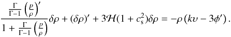$\frac{\frac{Γ}{Γ - 1} {(\frac{p}{ρ})}^{'}}{1 + \frac{Γ}{Γ - 1} (\frac{p}{ρ})} δρ + {(δρ)}^{'} + 3 ℋ (1 + c_{s}^{2}) δρ = - ρ (kυ - 3 φ^{'}) .$ $\begin{equation} \frac{\frac{\Gm}{\Gm - 1} \left ( \frac{p}{\rh} \right )^{\prime}}{1 + \frac{\Gm}{\Gm - 1} \left ( \frac{p}{\rh} \right )} \dl \rh + \left ( \dl \rh \right )^{\prime} + 3 {\cal H} (1 + c_{\rm s}^2) \dl \rh = - \rh \left ( k \ups - 3 \phi^{\prime} \right ). \end{equation}$ (35)Upon consideration of Eqs. (30) and (31), we obtain 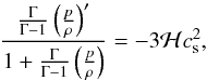$\frac{\frac{Γ}{Γ - 1} {(\frac{p}{ρ})}^{'}}{1 + \frac{Γ}{Γ - 1} (\frac{p}{ρ})} = - 3 ℋ c_{s}^{2},$ $\begin{equation} \frac{\frac{\Gm}{\Gm - 1} \left ( \frac{p}{\rh} \right )^{\prime}}{1 + \frac{\Gm}{\Gm - 1} \left ( \frac{p}{\rh} \right )} = - 3 {\cal H} c_{\rm s}^2, \end{equation}$ (36)where 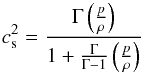$c_{s}^{2} = \frac{Γ (\frac{p}{ρ})}{1 + \frac{Γ}{Γ - 1} (\frac{p}{ρ})}$ $\begin{equation} c_{\rm s}^2 = \frac{\Gm \left ( \frac{p}{\rh} \right )}{1 + \frac{\Gm}{\Gm - 1} \left ( \frac{p}{\rh} \right )} \end{equation}$ (37)is the (polytropic) speed of sound (cf. Eq. (85) of Kleidis & Spyrou 2015), so that Eq. (35) is written in the form ${(δρ)}^{'} + 3 ℋ δρ = - ρ (kυ - 3 φ^{'}) .$ $\begin{equation} \left ( \dl \rh \right )^{\prime} + 3 {\cal H} \dl \rh = - \rh \left ( k \ups - 3 \phi^{\prime} \right ). \end{equation}$ (38)Finally, taking (once again) Eq. (30) into account and defining the density contrast, δ, as $δ = \frac{δρ}{ρ}$ $\hbox{$\dl = \frac{\dl \rh}{\rh}$}$ , Eq. (38) results in 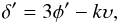$δ^{'} = 3 φ^{'} - kυ,$ $\begin{equation} \dl^{\prime} = 3 \phi^{\prime} - k \ups, \end{equation}$ (39)which is identical to Eq. (3.107) of Knobel (2012).

In the same fashion, upon consideration of Eqs. (30) and (36), the combination of Eqs. (26) and (33) yields 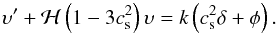$υ^{'} + ℋ (1 - 3 {c_{s}^{2}}^{)} υ = k (c_{s}^{2} δ + φ^{)} .$ $\begin{equation} \ups^{\prime} + {\cal H} \left ( 1 - 3 c_{\rm s}^2 \right ) \ups = k \left ( c_{\rm s}^2 \dl + \phi \right ). \end{equation}$ (40)Now, differentiating Eq. (39) and combining the outcome with Eq. (40), we obtain 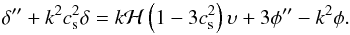$δ^{′′} + k^{2} c_{s}^{2} δ = k ℋ (1 - 3 {c_{s}^{2}}^{)} υ + 3 φ^{′′} - k^{2} φ .$ $\begin{equation} \dl^{\prime \prime} + k^2 c_{\rm s}^2 \dl = k {\cal H} \left ( 1 - 3 c_{\rm s}^2 \right ) \ups + 3 \phi^{\prime \prime} - k^2 \phi. \end{equation}$ (41)Finally, we may (re)use Eq. (39) to eliminate υ from the rhs of Eq. (41), which in this case results in 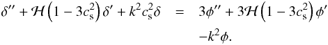$\begin{matrix} δ^{′′} + ℋ (1 - 3 {c_{s}^{2}}^{)} δ^{'} + k^{2} c_{s}^{2} δ & = & 3 φ^{′′} + 3 ℋ (1 - 3 {c_{s}^{2}}^{)} φ^{'} \\ - k^{2} φ . \end{matrix}$ $\begin{eqnarray} \dl^{\prime \prime} + {\cal H} \left ( 1 - 3 c_{\rm s}^2 \right ) \dl^{\prime} + k^2 c_{\rm s}^2 \dl & = & 3 \phi^{\prime \prime} + 3 {\cal H} \left ( 1 - 3 c_{\rm s}^2 \right ) \phi^{\prime} \nn \\ && - k^2 \phi. \end{eqnarray}$ (42)For $c_{s}^{2} = 0$ $\hbox{$c_{\rm s}^2 = 0$}$ , Eq. (42) reduces to Eq. (3.109) of Knobel (2012), that governs the evolution of conventional (i.e., pressureless) CDM perturbations in an expanding spatially flat cosmological model.

Equation (42) is an inhomogeneous second-order differential equation that governs the propagation of rest-mass density perturbations in the presence of the source term $S (η) = 3 [φ^{′′} + ℋ (1 - 3 {c_{s}^{2}}^{)} φ^{'} - \frac{k^{2}}{3} φ],$ $\begin{equation} S (\et) = 3 \left [ \phi^{\prime \prime} + {\cal H} \left ( 1 - 3 c_{\rm s}^2 \right ) \phi^{\prime} - \frac{k^2}{3} \phi \right ], \end{equation}$ (43)which depends on the generalized Newtonian potential, φ.

To determine the functional form of φ (and, hence, of S(η), as well), we note that the combination of Eqs. (24) and (33) yields $φ^{′′} + 3 ℋ φ^{'} + (2 ℋ^{'} + ℋ^{2}) φ = Γ (\frac{p}{ρ}) (4 πG R^{2} δ ρ^{)},$ $\begin{equation} \phi^{\prime \prime} + 3 {\cal H} \phi^{\prime} + \left ( 2 {\cal H}^{\prime} + {\cal H}^2 \right ) \phi = \Gm \left ( \frac{p}{\rh} \right ) \left ( 4 \pi G R^2 \dl \rh \right ), \end{equation}$ (44)while the combination of Eqs. (22) and (34) results in $- [k^{2} φ + 3 ℋ {(φ^{'} + ℋ φ)}^{]} = [1 + \frac{Γ}{Γ - 1} (\frac{p}{ρ})] (4 πG R^{2} δ ρ^{)} .$ $\begin{equation} - \left [ k^2 \phi + 3 {\cal H} \left ( \phi^{\prime} + {\cal H} \phi \right ) \right ] = \left [ 1 + \frac{\Gm}{\Gm - 1} \left ( \frac{p}{\rh} \right ) \right ] \left ( 4 \pi G R^2 \dl \rh \right ). \end{equation}$ (45)Now, Eqs. (44) and (45) can be combined with each other, to give $\begin{matrix} φ^{′′} + 3 ℋ φ^{'} + (2 ℋ^{'} + ℋ^{2}) φ = \\ - \frac{Γ (\frac{p}{ρ})}{1 + \frac{Γ}{Γ - 1} (\frac{p}{ρ})} [k^{2} φ + 3 ℋ {(φ^{'} + ℋ φ)}^{]}, \end{matrix}$ $\begin{eqnarray} && \phi^{\prime \prime} + 3 {\cal H} \phi^{\prime} + \left ( 2 {\cal H}^{\prime} + {\cal H}^2 \right ) \phi \nn =\\ & & \qquad - \frac{\Gm \left ( \frac{p}{\rh} \right )}{ 1 + \frac{\Gm}{\Gm - 1} \left ( \frac{p}{\rh} \right )} \left [ k^2 \phi + 3 {\cal H} \left ( \phi^{\prime} + {\cal H} \phi \right ) \right ], \end{eqnarray}$ (46)which in view of Eq. (37), can be written in the more convenient form $φ^{′′} + 3 ℋ (1 + {c_{s}^{2}}^{)} φ^{'} + [k^{2} c_{s}^{2} + 2 ℋ^{'} + (1 + 3 {c_{s}^{2}}^{)} ℋ^{2}] φ = 0.$ $\begin{equation} \phi^{\prime \prime} + 3 {\cal H} \left ( 1 + c_{\rm s}^2 \right ) \phi^{\prime} + \left [ k^2 c_{\rm s}^2 + 2 {\cal H}^{\prime} + \left ( 1 + 3 c_{\rm s}^2 \right ) {\cal H}^2 \right ] \phi = 0. \end{equation}$ (47)Equation (47) coincides with Eq. (7.51) of Mukhanov (2005), which drives the isentropic $\hbox{$(\dl {\cal S} = 0)$}$ evolution of metric perturbations in an expanding, spatially flat spacetime.

For Γ ≠ 0, given the appropriate initial conditions, the solution, {φ,δ,υ}, to the set of simultaneous differential Eqs. (40), (42), and (47) fully determines the evolution of cosmological perturbations in the polytropic DM model under consideration. Now, the only equation that has not been used, that is, Eq. (23), may serve as a constraint on the exact functional form of {φ,δ,υ}. However, an analytic solution to the system of Eqs. (40), (42) and (47) is rather hard to obtain; this is the scope of a future work. Accordingly, in order to take a first glance at the problem of cosmological perturbations in a polytropic DM model, we focus our attention below on its ΛCDM-like limit, that is, on the case where $Γ = 0 (= c_{s}^{2})$ $\hbox{$\Gm = 0 ~ ( {=}c_{\rm s}^2 )$}$ .

4. Reduction to the ΛCDM-like limit

For Γ = 0, we have p = const. = − | p₀ | < 0 and δp = 0 (cf. Eqs. (1), (8) and (33)). In this case, in order to track the evolution of cosmological perturbations, we begin with the field Eqs. (22)–(24). For Γ = 0, Eqs. (22) and (24) decouple because now, Eq. (24) is written in the form $φ^{′′} + 3 ℋ φ^{'} + (2 ℋ^{'} + ℋ^{2}) φ = 0,$ $\begin{equation} \phi^{\prime \prime} + 3 {\cal H} \phi^{\prime} + \left ( 2 {\cal H}^{\prime} + {\cal H}^2 \right ) \phi = 0, \end{equation}$ (48)which upon consideration of Eqs. (27) and (28), results in $φ^{′′} + 3 ℋ φ^{'} - 8 πG p_{0} R^{2} φ = 0.$ $\begin{equation} \phi^{\prime \prime} + 3 {\cal H} \phi^{\prime} - 8 \pi G p_0 R^2 \phi = 0. \end{equation}$ (49)On the other hand, by virtue of Eq. (34), Eq. (22) reads $δρ = - \frac{1}{4 πG R^{2}} [k^{2} φ + 3 ℋ {(φ^{'} + ℋ φ)}^{]} .$ $\begin{equation} \dl \rh = - \frac{1}{4 \pi G R^2} \left [ k^2 \phi + 3 {\cal H} \left ( \phi^{\prime} + {\cal H} \phi \right ) \right ]. \end{equation}$ (50)Clearly, in order to determine the evolution of rest-mass density perturbations, δρ, we first of all need to solve Eq. (49), which drives the dynamics of φ.

To do so, in Eq. (49), we change the independent variable from conformal time, dη, to its cosmic counterpart, dt = Rdη, yielding $\begin{matrix} ¨ \\ φ \end{matrix} + 4 H φ̇ - 8 πG p_{0} φ = 0,$ $\begin{equation} \ddot{\phi} + 4 H \dot{\phi} - 8 \pi G p_0 \phi = 0 , \end{equation}$ (51)and once again, this time from cosmic time, t, to cosmological redshift, z, as follows $w = 1 + z = \frac{R_{0}}{R (t)},$ $\begin{equation} w = 1 + z = \frac{R_0}{R (t)}, \end{equation}$ (52)yielding, $\begin{matrix} φ̇ & = & - wH \frac{d φ}{d w} and \\ \begin{matrix} ¨ \\ φ \end{matrix} & = & w H^{2} \frac{d φ}{d w} + \frac{1}{2} w^{2} \frac{d (H^{2})}{d w} \frac{d φ}{d w} + w^{2} H^{2} \frac{d^{2} φ}{d w^{2}} \cdot \end{matrix}$ $\begin{eqnarray} \dot{\phi} & =& - w H \frac{{\rm d} \phi}{{\rm d} w} ~~~\mbox{and} \nn \\ \ddot{\phi} & =& w H^2 \frac{{\rm d} \phi}{{\rm d} w} + \frac{1}{2} w^2 \frac{{\rm d} \left ( H^2 \right )}{{\rm d} w} \frac{{\rm d} \phi}{{\rm d} w} + w^2 H^2 \frac{{\rm d}^2 \phi}{{\rm d} w^2}\cdot \end{eqnarray}$ (53)Now, in terms of w, Eq. (51) is written in the form $\frac{d^{2} φ}{d w^{2}} + [\frac{1}{2 H^{2}} \frac{d (H^{2})}{d w} - \frac{3}{w}] \frac{d φ}{d w} - \frac{8 πG p_{0}}{w^{2} H^{2}} φ = 0.$ $\begin{equation} \frac{{\rm d}^2 \phi}{{\rm d} w^2} + \left [ \frac{1}{2 H^2} \frac{{\rm d} \left ( H^2 \right )}{{\rm d} w} - \frac{3}{w} \right ] \frac{ {\rm d} \phi}{{\rm d} w} - \frac{8 \pi G p_0}{w^2 H^2} \phi = 0. \end{equation}$ (54)In view of Eq. (9), in the ΛCDM-like (Γ = 0) limit of the polytropic DM model under consideration, the Hubble parameter is given by $H^{2} = H_{0}^{2} [Ω_{M} w^{3} + {(1 - Ω_{M})}^{]},$ $\begin{equation} H^2 = H_0^2 \left [ \Om_{\rm M} w^3 + \left ( 1 - \Om_{\rm M} \right ) \right ], \end{equation}$ (55)so that eventually, Eq. (54) results in $\begin{matrix} \frac{d^{2} φ}{d w^{2}} & + & [\frac{3 / 2}{w} \frac{1}{(1 + \frac{1 - Ω_{M}}{Ω_{M}} {\frac{1}{w^{3}}}^{)}} - \frac{3}{w}] \frac{d φ}{d w} \\ - & \frac{8 πG p_{0}}{Ω_{M} H_{0}^{2}} \frac{1}{w^{5}} \frac{1}{(1 + \frac{1 - Ω_{M}}{Ω_{M}} {\frac{1}{w^{3}}}^{)}} φ = 0. \end{matrix}$ $\begin{eqnarray} \frac{{\rm d}^2 \phi}{{\rm d}w^2} & + & \left [ \frac{3/2}{w} \frac{1}{\left( 1 + \frac{1 - \Om_{\rm M}}{\Om_{\rm M}} \frac{1}{w^3} \right )} - \frac{3}{w} \right ] \frac{{\rm d} \phi}{{\rm d} w} \nn \\ & - & \frac{8 \pi G p_0}{\Om_{\rm M} H_0^2} \frac{1}{w^5} \frac{1}{\left( 1 + \frac{1 - \Om_{\rm M}}{\Om_{\rm M}} \frac{1}{w^3} \right )} \phi = 0. \end{eqnarray}$ (56)At this point, we note that the w-span we are interested in to solve Eq. (56) falls into the range 101 ≤ w ≤ 1091, corresponding to values of cosmological redshift that range from recombination (z ≈ 1090) to z = 100, when, as is now consensus, the DM structures had already been formed (see, e.g., Naoz & Barkana 2005; Knobel 2012; see also Sandvik et al. 2004, for a slightly different explanation). When we once again assume that Ω_M = 0.308 (Planck Collaboration XIII 2016), for every z ≥ 100, the quantity $(w, Ω_{M}) = \frac{1 - Ω_{M}}{Ω_{M}} \frac{1}{w^{3}} \leq 2.2 \times 10^{-6} ≪ 1,$ $\begin{equation} \left ( w, \Om_{\rm M} \right ) = \frac{1 - \Om_{\rm M}}{\Om_{\rm M}} \frac{1}{w^3} \leq 2.2 \times 10^{-6} \ll 1, \end{equation}$ (57)is extremely small and can therefore be ignored as compared to unity. We note that such an approximation would be accurate enough even for z ≥ 11, that is, at every pre-reionization epoch, because then, (w,Ω_M) ≤ 1.3 × 10^-3 ≪ 1, as well. Accordingly, Eq. (56) is reduced to $\frac{d^{2} φ}{d w^{2}} - \frac{3 / 2}{w} \frac{d φ}{d w} + 3 \frac{| p_{0} |}{ρ_{0}} \frac{1}{w^{5}} φ = 0,$ $\begin{equation} \frac{{\rm d}^2 \phi}{{\rm d} w^2} - \frac{3/2}{w} \frac{{\rm d} \phi}{{\rm d} w} + 3 \frac{\vert p_0 \vert}{\rh_0} \frac{1}{w^5} \phi = 0, \end{equation}$ (58)where we have taken into account that in view of Eq. (23) of Kleidis & Spyrou (2015), we have $- \frac{8 πG p_{0}}{Ω_{M} H_{0}^{2}} = 3 \frac{| p_{0} |}{ρ_{0}} [= 3 \frac{1 - Ω_{M}}{Ω_{M}}] \cdot$ $\begin{equation} - \frac{8 \pi G p_0}{\Om_{\rm M} H_0^2} = 3 \frac{\vert p_0 \vert}{\rh_0} \left [ = 3 \frac{1 - \Om_{\rm M}}{\Om_{\rm M}} \right ]\cdot \end{equation}$ (59)Equation (58) admits the solution 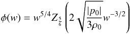$φ (w) = w^{5 / 4} Z_{\frac{5}{6}} (2 \sqrt{\frac{| p_{0} |}{3 ρ_{0}}} w^{- 3 / 2})$ $\begin{equation} \phi (w) = w^{5/4} Z_{\frac{5}{6}} \left ( 2 \sqrt{\frac{\vert p_0 \vert}{3 \rh_0}} w^{-3/2} \right ) \end{equation}$ (60)(see, e.g., Gradshteyn & Ryzhik 2007, Eq. (8.491.12)), where 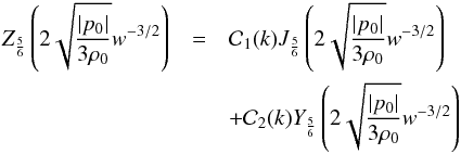$\begin{matrix} Z_{\frac{5}{6}} (2 \sqrt{\frac{| p_{0} |}{3 ρ_{0}}} w^{- 3 / 2}) & = & 𝒞_{1} (k) J_{\frac{5}{6}} (2 \sqrt{\frac{| p_{0} |}{3 ρ_{0}}} w^{- 3 / 2}) \\ + 𝒞_{2} (k) Y_{\frac{5}{6}} (2 \sqrt{\frac{| p_{0} |}{3 ρ_{0}}} w^{- 3 / 2}) \end{matrix}$ $\begin{eqnarray} Z_{\frac{5}{6}} \left ( 2 \sqrt{\frac{\vert p_0 \vert}{3 \rh_0}} w^{-3/2} \right ) & =& {\cal C}_1 (k) J_{\frac{5}{6}} \left ( 2 \sqrt{\frac{\vert p_0 \vert}{3 \rh_0}} w^{-3/2} \right ) \nn \\ & &+ {\cal C}_2 (k) Y_{\frac{5}{6}} \left ( 2 \sqrt{\frac{\vert p_0 \vert}{3 \rh_0}} w^{-3/2} \right ) \end{eqnarray}$ (61)is the linear combination of Bessel functions of the first, J_ν, and the second, Y_ν, kind, on the order of $ν = \frac{5}{6}$ $\hbox{$\nu = \frac{5}{6}$}$ , and $\hbox{${\cal C}_1 (k)$}$ , $\hbox{${\cal C}_2 (k)$}$ are (complex) constants. On physical grounds, we admit that $\hbox{${\cal C}_2 (k) = 0$}$ , otherwise, at large z, we would have φ → ∞, which is not anticipated, not even by inflationary cosmology (see, e.g., Linde 1990). In this case, at high values of w, the argument (~ w^{− 3 / 2}) of the only Bessel function left, $J_{\frac{5}{6}}$ $\hbox{$J_{\frac{5}{6}}$}$ , diminishes, so that 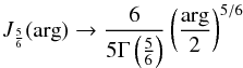$J_{\frac{5}{6}} (\arg) \to \frac{6}{5 Γ ({\frac{5}{6}}^{)}} {(\frac{\arg}{2})}^{5 / 6}$ $\begin{equation} J_{\frac{5}{6}} (\arg) \rarrow \frac{6}{5 \Gm \left ( \frac{5}{6} \right )} \left ( \frac{\arg}{2} \right )^{5/6} \end{equation}$ (62)(see, e.g., Olver et al. 2010, Eq. (10.7.3)), where $Γ {}^{(}{\frac{5}{6}}^{)} = 1.12879$ $\hbox{$\Gm \left ( \frac{5}{6} \right ) = 1.12879$}$ is Euler’s Gamma function of argument equal to $\frac{5}{6}$ $\hbox{$\frac{5}{6}$}$ . Accordingly, 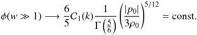$φ (w ≫ 1) - \to \frac{6}{5} 𝒞_{1} (k) \frac{1}{Γ ({\frac{5}{6}}^{)}} {(\frac{| p_{0} |}{3 ρ_{0}})}^{5 / 12} = const .$ $\begin{equation} \phi (w \gg 1) \longrightarrow \frac{6}{5} {\cal C}_1 (k) \frac{1}{\Gm \left ( \frac{5}{6} \right ) } \left ( \frac{ \vert p_0 \vert}{3 \rh_0} \right )^{5/12} = \textrm{const.} \end{equation}$ (63)The amplitude of metric perturbations, | φ |, normalized over $\hbox{$\vert {\cal C}_1 (k) \vert$}$ , as a function of w, is given in Fig. 2. We note that for z ≥ 100, we have | φ | ≈ const., in complete correspondence to Eq. (63). In this way, the solution given by Eq. (60) justifies the scientific perception that in the early matter-dominated era, metric perturbations were (more or less) constant (see, e.g., Knobel 2012).

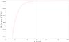Fig. 2

Amplitude of the generalized Newtonian potential, | φ |, normalized over $\hbox{$\vert {\cal C}_1 (k) \vert$}$ , as a function of w = 1 + z. It is evident that for w ≥ 100, | φ | = const. to high accuracy.

Now, by virtue of Eq. (60), Eq. (50) exhibits the evolution of rest-mass density perturbations in terms of w = 1 + z, namely, $δρ = \frac{1}{4 πG} [3 w H^{2} \frac{d φ}{d w} - {({k_{0}^{ph}}^{)}}^{2} w^{2} φ - 3 H^{2} φ],$ $\begin{equation} \dl \rh = \frac{1}{4 \pi G} \left [ 3 w H^2 \frac{{\rm d} \phi}{{\rm d} w} - \left ( k_0^{\rm ph} \right )^2 w^2 \phi - 3 H^2 \phi \right ], \end{equation}$ (64)where we have defined the physical wavenumber at the present epoch, $k_{0}^{ph}$ $\hbox{$k_0^{\rm ph}$}$ , as $k_{0}^{ph} = \frac{k}{R_{0}}$ $\hbox{$k_0^{\rm ph} = \frac{k}{R_0}$}$ . Inserting Eq. (55) into (64) and taking condition (57) into account, we obtain $δρ = 2 ρ_{0} [w^{4} \frac{d φ}{d w} - \frac{1}{3 Ω_{M}} {(\frac{k_{0}^{ph}}{H_{0}})}^{2} w^{2} φ - w^{3} φ],$ $\begin{equation} \dl \rh = 2 \rh_0 \left [ w^4 \frac{{\rm d} \phi}{{\rm d} w} - \frac{1}{3 \Om_{\rm M}} \left ( \frac{k_0^{\rm ph}}{H_0} \right )^2 w^2 \phi - w^3 \phi \right ], \end{equation}$ (65)where, in view of Eq. (23) of Kleidis & Spyrou (2015), we have set $8 πG ρ_{0} = 3 Ω_{M} H_{0}^{2}$ $\hbox{$8 \pi G \rh_0 = 3 \Om_{\rm M} H_0^2$}$ . We note that in Eq. 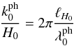(65), the quantity $\frac{k_{0}^{ph}}{H_{0}} = 2 π \frac{ℓ_{H_{0}}}{λ_{0}^{ph}}$ $\begin{equation} \frac{k_0^{\rm ph}}{H_0} = 2 \pi \frac{\ell_{H_0}}{\lm_0^{\rm ph}} \end{equation}$ (66)is a measure of the number of potential structures (each one of linear dimension $λ_{0}^{ph}$ $\hbox{$\lm_0^{\rm ph}$}$ ) inside the disk of present-time (Hubble) radius $ℓ_{H_{0}} = \frac{1}{H_{0}} \approx 4.28$ $\hbox{$\ell_{H_0} = \frac{1}{H_0} \approx 4.28$}$ Gpc. Depending on the linear dimensions of the various structures observed today, the number given by Eq. (66) may vary from the order of ten (e.g., as regards galaxy filaments) to 10⁵ (as regards structures of linear dimensions comparable to those of individual galaxies). Clearly, the smaller the linear dimensions of a particular perturbation scale, the more numerous its representatives at the present epoch.

Finally, by dividing both parts of Eq. (65) by ρ and taking into account Eq. (5), we find that the rest-mass density contrast, $δ = \frac{δρ}{ρ}$ $\hbox{$\dl = \frac{\dl \rh}{\rh}$}$ , is related to metric perturbation, φ, as $δ = 2 [w \frac{d φ}{d w} - \frac{1}{3 Ω_{M}} {(\frac{k_{0}^{ph}}{H_{0}})}^{2} \frac{1}{w} φ - φ] .$ $\begin{equation} \dl = 2 \left [ w \frac{{\rm d} \phi}{{\rm d}w} - \frac{1}{3 \Om_{\rm M}} \left ( \frac{k_0^{\rm ph}}{H_0} \right )^2 \frac{1}{w} \phi - \phi \right ] . \end{equation}$ (67)Upon consideration of Eqs. (60) and (61), and taking into account Eq. (8.472.2) of Gradshteyn & Ryzhik (2007), Eq. (67) results in $\begin{matrix} δ & = & \frac{2}{w^{1 / 4}} 𝒞_{1} (k) [\sqrt{\frac{3 | p_{0} |}{ρ_{0}}} J_{\frac{11}{6}} (2 \sqrt{\frac{| p_{0} |}{3 ρ_{0}}} w^{- 3 / 2}) \\ - \frac{1}{3 Ω_{M}} {(\frac{k_{0}^{ph}}{H_{0}})}^{2} w^{1 / 2} J_{\frac{5}{6}} {(2 \sqrt{\frac{| p_{0} |}{3 ρ_{0}}} w^{- 3 / 2})}^{} \\ - w^{3 / 2} J_{\frac{5}{6}} (2 \sqrt{\frac{| p_{0} |}{3 ρ_{0}}} w^{- 3 / 2})] . \end{matrix}$ $\begin{eqnarray} \dl &=& \frac{2}{w^{1/4}} {\cal C}_1 (k) \left [ \sqrt{\frac{3 \vert p_0 \vert}{\rh_0}} J_{\frac{11}{6}} \left ( 2 \sqrt{\frac{\vert p_0 \vert}{3 \rh_0}} w^{-3/2} \right ) \right . \nn \\[1.5mm] & & - \left. \frac{1}{3 \Om_{\rm M}} \left ( \frac{k_0^{\rm ph}}{H_0} \right )^2 w^{1/2} J_{\frac{5}{6}} \left ( 2 \sqrt{\frac{\vert p_0 \vert}{3 \rh_0}} w^{-3/2} \right ) \right. \nn \\[1.5mm] & & -\left. w^{3/2} J_{\frac{5}{6}} \left ( 2 \sqrt{\frac{\vert p_0 \vert}{3 \rh_0}} w^{-3/2} \right ) \right ] . \end{eqnarray}$ (68)At large z(w ≫ 1), upon consideration of the constraint (57) and Eq. (62), we obtain $\begin{matrix} δ (w ≫ 1) & - \to & 2 𝒞_{1} (k) \frac{1}{Γ ({\frac{11}{6}}^{)}} {(\frac{| p_{0} |}{3 ρ_{0}})}^{5 / 12} \\ \times [1 + \frac{1}{3 Ω_{M}} {(\frac{k_{0}^{ph}}{H_{0}})}^{2} \frac{1}{w}] \cdot \end{matrix}$ $\begin{eqnarray} \dl (w \gg 1) & \longrightarrow & 2 {\cal C}_1 (k) \frac{1}{\Gm \left ( \frac{11}{6} \right ) } \left ( \frac{ \vert p_0 \vert}{3 \rh_0} \right )^{5/12} \nn \\[1.5mm] && \times \left [ 1 + \frac{1}{3 \Om_{\rm M}} \left ( \frac{k_0^{\rm ph}}{H_0} \right )^2 \frac{1}{w} \right ] \cdot \end{eqnarray}$ (69)Now, there are two points worth noting in connection with Eq. (69).

First, for small-scale structures (from the cosmological point of view), $(\frac{k_{0}^{ph}}{H_{0}}) ≫ 1$ $\hbox{$ \left(\frac{k_0^{\rm ph}}{H_0}\right) \gg 1$}$ , meaning that the second term in brackets on the rhs of Eq. (69) is dominant for every w. In contrast, for $k_{0}^{ph} \approx H_{0}$ $\hbox{$k_0^{\rm ph} \approx H_0$}$ , that is, for the very large-scale structures we see today (e.g., the Hercules – Corona Borealis Great Wall, a huge filament measuring more than 10¹⁰ light years across, Horvath et al. 2013), this term is suppressed at high values of w, as w^-1. Figure 3 shows that the longer the present timescale of a structure, the lower the growth rate (and the amplitude) of the associated perturbation mode. In other words, according to the polytropic approach to a ΛCDM-like model, creation of the large-scale structures we see today is disfavored at early times (at high values of w), suggesting that small-scale structures must have been formed first, aggregating to form larger structures later; this is exactly what the CDM scenario implies.

Fig. 3

Amplitude of the rest-mass density contrast, | δ |, normalized over $\hbox{$\vert {\cal C}_1 (k) \vert$}$ , as a function of the Universe scale factor, R, for $(\frac{k_{0}^{ph}}{H_{0}}) = 10$ $\hbox{$\left( \frac{k_0^{\rm ph}}{H_0} \right) = 10$}$ (blue solid line), and 100 (red solid line). The vertical dashed line marks the recombination epoch. We observe that the longer the present timescale of a structure, the more suppressed the associated perturbation mode.

The second point is that at every post-recombination epoch (z< 1090), to leading order in $(\frac{k_{0}^{ph}}{H_{0}})$ $\hbox{$\left(\frac{k_0^{\rm ph}}{H_0}\right)$}$ (i.e., for small-scale perturbation modes), Eq. (69) is reduced to $δ ~ w^{-1} ~ R .$ $\begin{equation} \dl \sim w^{-1} \sim R . \end{equation}$ (70)In view of Eq. (70), the evolution of matter perturbations in the ΛCDM-like limit of the polytropic-DM model under consideration also conforms with the so-called Meszaros effect (Meszaros 1974), which is considered to govern the evolution of cosmological perturbations during the matter-dominated epoch; namely, the rest-mass density contrast grows smoothly, being proportional to the Universe scale factor, R (cf. Fig. 3). We note that this effect applies much more accurately to small-scale structures for which $(\frac{k_{0}^{ph}}{H_{0}}) ≫ 1$ $\hbox{$\left( \frac{k_0^{\rm ph}}{H_0} \right) \gg 1$}$ . For $(\frac{k_{0}^{ph}}{H_{0}}) = 1000$ $\hbox{$\left( \frac{k_0^{\rm ph}}{H_0} \right) = 1000$}$ , | δ | ~ R^0.995, while for $(\frac{k_{0}^{ph}}{H_{0}}) = 10$ $\hbox{$\left( \frac{k_0^{\rm ph}}{H_0} \right) = 10$}$ , | δ | ~ R^0.945 (cf. Fig. 4).

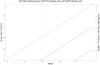Fig. 4

Amplitude of the rest-mass density contrast, | δ |, in units of $\hbox{$\vert {\cal C}_1 (k) \vert$}$ , as a function of the Universe scale factor, R, for $(\frac{k_{0}^{ph}}{H_{0}}) = 10$ $\hbox{$\left( \frac{k_0^{\rm ph}}{H_0} \right) = 10$}$ (blue solid line), 100 (red solid line), and 1000 (green solid line). The vertical dashed line marks the onset of matter-dominated era, in which our (linear) perturbative analysis holds. We observe that for z< 1090, polytropic DM perturbations conform with the Meszaros effect (i.e., δ ~ R) to high accuracy.

Finally, by virtue of Eq. (60), we may also determine the comoving counterpart, υ, of the peculiar velocity field, υ_pec = υR. To do so, we first express Eq. (23) in terms of w to obtain $υ = \frac{2}{3} \frac{1}{\sqrt{Ω_{M}}} (\frac{k_{0}^{ph}}{H_{0}}) \frac{1}{\sqrt{w}} (φ - w \frac{d φ}{d w}),$ $\begin{equation} \ups = \frac{2}{3} \frac{1}{\sqrt{\Om_{\rm M}}} \left ( \frac{k_0^{\rm ph}}{H_0} \right ) \frac{1}{\sqrt{w}} \left ( \phi - w \frac{{\rm d} \phi}{{\rm d}w} \right ), \end{equation}$ (71)where once again, we have taken into account Eq. (57). Upon consideration of Eq. (60), Eq. (71) results in $\begin{matrix} υ & = & \frac{2}{3} 𝒞_{1} (k) \frac{1}{\sqrt{Ω_{M}}} (\frac{k_{0}^{ph}}{H_{0}}) \frac{1}{w^{5 / 4}} [w^{2} J_{\frac{5}{6}} (2 \sqrt{\frac{| p_{0} |}{3 ρ_{0}}} w^{- 3 / 2}) \\ - \sqrt{\frac{3 | p_{0} |}{ρ_{0}}} J_{\frac{11}{6}} (2 \sqrt{\frac{| p_{0} |}{3 ρ_{0}}} w^{- 3 / 2})] . \end{matrix}$ $\begin{eqnarray} \ups & = & \frac{2}{3} {\cal C}_1 (k) \frac{1}{\sqrt{\Om_{\rm M}}} \left ( \frac{k_0^{\rm ph}}{H_0} \right ) \frac{1}{w^{5/4}} \left [ w^2 J_{\frac{5}{6}} \left ( 2 \sqrt{\frac{\vert p_0 \vert}{3 \rh_0}} w^{-3/2} \right ) \right. \nn \\ & &- \left. \sqrt{\frac{3 \vert p_0 \vert}{\rh_0}} J_{\frac{11}{6}} \left ( 2 \sqrt{\frac{\vert p_0 \vert}{3 \rh_0}} w^{-3/2} \right ) \right ] . \end{eqnarray}$ (72)By virtue of Eq. (62), in the early matter-dominated era (i.e., for w ≫ 1), the peculiar velocity (72) of the perturbation mode denoted by k(υ ≡ υ_k) is reduced to $υ_{k} \to \frac{4}{5} 𝒞_{1} (k) \frac{1}{\sqrt{Ω_{M}}} (\frac{k_{0}^{ph}}{H_{0}}) \frac{1}{Γ ({\frac{5}{6}}^{)}} {(\frac{| p_{0} |}{3 ρ_{0}})}^{\frac{5}{12}} \frac{1}{\sqrt{w}} \cdot$ $\begin{equation} \ups_k \rarrow \frac{4}{5} {\cal C}_1 (k) \frac{1}{\sqrt{\Om_{\rm M}}} \left ( \frac{k_0^{\rm ph}}{H_0} \right ) \frac{1}{\Gm \left ( \frac{5}{6} \right )} \left ( \frac{\vert p_0 \vert}{3 \rh_0} \right )^{\frac{5}{12}} \frac{1}{\sqrt{w}} \cdot \end{equation}$ (73)The average velocity of all perturbation modes inside the Hubble radius can be defined as $⟨ υ_{pec} ⟩ = \lim_{k \to \infty} \frac{1}{k - H} \int_{H}^{k} υ_{k^{'}} d k^{'},$ $\begin{equation} \langle \ups_{\rm pec} \rangle = \lim_{k \rarrow \infty} \frac{1}{k - H} \int_H^k \ups_{k^{\prime}} {\rm d} k^{\prime}, \end{equation}$ (74)which upon consideration of Eq. (74), yields 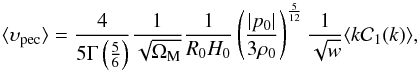$⟨ υ_{pec} ⟩ = \frac{4}{5 Γ ({\frac{5}{6}}^{)}} \frac{1}{\sqrt{Ω_{M}}} \frac{1}{R_{0} H_{0}} {(\frac{| p_{0} |}{3 ρ_{0}})}^{\frac{5}{12}} \frac{1}{\sqrt{w}} ⟨ k 𝒞_{1} (k) ⟩,$ $\begin{equation} \langle \ups_{\rm pec} \rangle = \frac{4}{5 \Gm \left ( \frac{5}{6} \right )} \frac{1}{\sqrt{\Om_{\rm M}}} \frac{1}{R_0 H_0} \left ( \frac{\vert p_0 \vert}{3 \rh_0} \right )^{\frac{5}{12}} \frac{1}{\sqrt{w}} \langle k {\cal C}_1 (k) \rangle, \end{equation}$ (75)where the (average) value $\hbox{$\langle k {\cal C}_1 (k) \rangle$}$ is determined along the lines of Eq. (74). In view of Eq. (75), because of the non-zero polytropic pressure (p₀ ≠ 0), the comoving peculiar velocities are no longer redshifted away by cosmic expansion (i.e., by Hubble drag) as is predicted by conventional (i.e., pressureless) structure formation theory (see, e.g., Peacock 1999; Sparke & Ghallagher 2007). Instead, on descending values of w, ⟨ υ_pec ⟩ increases as 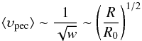$⟨ υ_{pec} ⟩ ~ \frac{1}{\sqrt{w}} ~ {(\frac{R}{R_{0}})}^{1 / 2}$ $\begin{equation} \langle \ups_{\rm pec} \rangle \sim \frac{1}{\sqrt{w}} \sim \left ( \frac{R}{R_0} \right )^{1/2} \end{equation}$ (76)(cf. Fig. 5). This result might be a suitable tool for either conceding or rejecting the polytropic DM model under consideration (at least, its ΛCDM-like limit). In fact, for | p | = const. = | p₀ | and ρ ~ R^-3, Eq. (76) is in complete correspondence to Eq. (14) regarding the evolution of comoving peculiar velocities in a cosmological model with thermodynamical content. This result suggests that in the linear regime, peculiar velocities of the small-scale CDM concentrations conform with the (non-relativistic) rms-velocity law of conventional statistical physics, given by Eq. (13). It is worth noting that although ⟨ υ_pec ⟩ increases, it still remains conveniently small, for example, for z ≥ 100, ⟨ υ_pec ⟩ ≤ 1.3 × 10^-3 ≪ 1 (cf. Eq. (13)). ⟨ υ_pec ⟩ < 1 at all cosmological redshifts higher than a particular value, 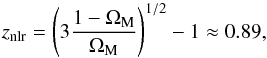$z_{nlr} = {(3 \frac{1 - Ω_{M}}{Ω_{M}})}^{1 / 2} - 1 \approx 0.89,$ $\begin{equation} z_{\rm nlr} = \left ( 3 \frac{1 - \Om_{\rm M}}{\Om_{\rm M}} \right )^{1/2} - 1 \approx 0.89, \end{equation}$ (77)where the suffix “nlr” stands for “non-linear regime”. z_nlr can be considered to represent the far outer edge of the linear regime (lying safely outside the ΛCDM-oriented acceleration era, which commences at z_tr ≈ 0.65, Planck Collaboration XIII 2016).

We also note that the larger the linear dimensions of a particular type of structures at the present epoch, the slower the peculiar velocity of the corresponding perturbations. For instance, at z = 4 (vertical dashed line in Fig. 5), perturbations on the order of $(\frac{k_{0}^{ph}}{H_{0}}) = 1000$ $\hbox{$\left( \frac{k_0^{ ph}}{H_0}\right) = 1000$}$ (i.e., of linear dimensions comparable to those of the Coma Cluster at the present epoch) were moving at a three times higher speed than those of linear dimensions on the order of present-time galaxy superclusters, that is, of $(\frac{k_{0}^{ph}}{H_{0}}) = 100$ $\hbox{$\left( \frac{k_0^{\rm ph}}{H_0} \right) = 100$}$ (cf. horizontal dashed lines in Fig. 5). This result might also be traced observationally, for example, by the forthcoming Euclid mission¹.

Fig. 5

Average peculiar velocity field, ⟨ υ_pec ⟩, normalized over $\hbox{$\langle k {\cal C}_1 (k) \rangle$}$ , as a function of the Universe scale factor, R, for $(\frac{k_{0}^{ph}}{H_{0}}) = 100$ $\hbox{$\left( \frac{k_0^{\rm ph}}{H_0} \right) = 100$}$ (red solid line) and 1000 (green solid line). We observe that within the linear regime, peculiar velocities conform with the rms-velocity law of statistical physics (i.e., $⟨ υ ⟩ ~ \sqrt{R}$ $\hbox{$\langle \ups \rangle \sim \sqrt{R}$}$ ) given by Eq. (14). In both curves, the receding part arising for $\frac{R}{R_{0}} \geq 0.2$ $\hbox{$\frac{R}{R_0} \geq 0.2$}$ (z ≤ 4) signals the onset of deviations from the rms-velocity law due to the collapse of linear approximation and Hubble drag.

After we used the field Eqs. (22)–(24) to arrive at { φ,δ,υ }, the perturbed equations of motion given by Eqs. (25) and (26) may now serve as constraints to our solution. In this context, in terms of w, Eq. (25) is written in the form $\frac{d δ}{d w} = 3 \frac{d φ}{d w} + \frac{2}{3} \frac{1}{Ω_{M}} {(\frac{k_{0}^{ph}}{H_{0}})}^{2} \frac{1}{w^{2}} (φ - w \frac{d φ}{d w}),$ $\begin{equation} \frac{{\rm d} \dl}{{\rm d} w} = 3 \frac{{\rm d} \phi}{{\rm d} w} + \frac{2}{3} \frac{1}{\Om_{\rm M}} \left ( \frac{k_0^{\rm ph}}{H_0} \right )^2\frac{1}{w^2} \left ( \phi - w \frac{{\rm d} \phi}{{\rm d} w} \right ), \end{equation}$ (78)where we once again used Eq. (57). By virtue of Eq. (67), Eq. (78) results in $2 w \frac{d}{d w} (\frac{d φ}{d w}) - 3 \frac{d φ}{d w} = 0.$ $\begin{equation} 2 w \frac{\rm d}{{\rm d}w} \left ( \frac{{\rm d} \phi}{{\rm d}w} \right ) - 3 \frac{{\rm d} \phi}{{\rm d}w} = 0 . \end{equation}$ (79)In the same fashion, Eq. (26) yields $\frac{1}{3} w \frac{1}{\sqrt{Ω_{M}}} (\frac{k_{0}^{ph}}{H_{0}}) [2 w \frac{d}{d w} (\frac{d φ}{d w}) - 3 \frac{d φ}{d w}] = 0.$ $\begin{equation} \frac{1}{3} w \frac{1}{\sqrt{\Om_{\rm M}}} \left ( \frac{k_0^{\rm ph} }{H_0} \right ) \left [ 2 w \frac{\rm d}{{\rm d}w} \left ( \frac{{\rm d} \phi}{{\rm d}w} \right ) - 3 \frac{{\rm d} \phi}{{\rm d}w} \right ] = 0 . \end{equation}$ (80)Clearly, both constraints are reduced to one, and only one, namely, Eq. (79), which for φ = const. is identically valid. Admitting that φ ≠ const., we may use Eq. (60) to monitor the evolution of Eq. (79) in terms of w. The outcome is given in Fig. 6. We observe that for w ≥ 100, the constraint (79) is satisfied to high accuracy.

Fig. 6

Equation of motion (79), monitored over the time span corresponding to 50 ≤ w = 1 + z ≤ 1100. It is evident that for w ≥ 100, this constraint is valid to an accuracy higher than 1:10⁷.

5. Power spectrum of density perturbations

In an isotropic cosmological model, the dimensionless power spectrum of rest-mass density perturbations is defined as $Δ^{2} (δ) = \frac{1}{2 π^{2}} k^{3} | δ (k) | 2$ $\begin{equation} \Dl^2(\dl) = \frac{1}{2 \pi^2} k^3 \vert \dl(k) \vert^2 \end{equation}$ (81)(see, e.g., Peacock 1999), and in a similar manner, the corresponding spectrum of metric perturbations is given by 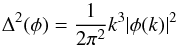$Δ^{2} (φ) = \frac{1}{2 π^{2}} k^{3} | φ (k) | 2$ $\begin{equation} \Dl^2(\phi) = \frac{1}{2 \pi^2} k^3 \vert \phi(k) \vert^2 \end{equation}$ (82)(see, e.g., Mukhanov 2005). Although there is no reason in principle why the rest-mass density spectrum should exhibit a power-law behavior (see, e.g., Liddle & Lyth 1993), it is commonly admitted that 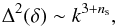$Δ^{2} (δ) ~ k^{3 + n_{s}},$ $\begin{equation} \Dl^2 (\dl) \sim k^{3 + n_{\rm s}}, \end{equation}$ (83)where n_s is the scalar spectral index (see, e.g., Knobel 2012). To calculate the spectrum of rest-mass density perturbations in the ΛCDM-like limit of the polytropic DM model under consideration, all we need is Eq. (67). In this context, we note that 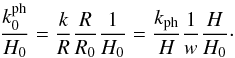$\frac{k_{0}^{ph}}{H_{0}} = \frac{k}{R} \frac{R}{R_{0}} \frac{1}{H_{0}} = \frac{k_{ph}}{H} \frac{1}{w} \frac{H}{H_{0}} \cdot$ $\begin{equation} \frac{k_0^{\rm ph}}{H_0} = \frac{k}{R} \frac{R}{R_0} \frac{1}{H_0} = \frac{k_{\rm ph}}{H} \frac{1}{w} \frac{H}{H_0} \cdot \end{equation}$ (84)Accordingly, $\begin{matrix} {(\frac{k_{0}^{ph}}{H_{0}})}^{2} & = & {(\frac{k_{ph}}{H})}^{2} \frac{1}{w^{2}} Ω_{M} w^{3} [1 + \frac{1 - Ω_{M}}{Ω_{M}} \frac{1}{w^{3}}] \\ ≃ & {(\frac{k_{ph}}{H})}^{2} Ω_{M} w, \end{matrix}$ $\begin{eqnarray} \left ( \frac{k_0^{\rm ph}}{H_0} \right )^2 & = & \left ( \frac{k_{\rm ph}}{H} \right )^2 \frac{1}{w^2} \Om_{\rm M} w^3 \left [ 1 + \frac{1 - \Om_{\rm M}}{\Om_{\rm M}} \frac {1}{w^3} \right ] \nn \\ & \simeq& \left ( \frac{k_{\rm ph}}{H} \right )^2 \Om_{\rm M} w, \end{eqnarray}$ (85)where we once again have taken into account Eq. (57). In view of Eq. (85), Eq. (67) is written in the form $δ = 2 [w \frac{d φ}{d w} - \frac{1}{3} {(\frac{k_{ph}}{H})}^{2} φ - φ] .$ $\begin{equation} \dl = 2 \left [ w \frac{{\rm d} \phi}{{\rm d}w} - \frac{1}{3} \left ( \frac{k_{\rm ph}}{H} \right )^2 \phi - \phi \right ] . \end{equation}$ (86)By virtue of Eq. (86), for φ ≈ const., we obtain $\frac{Δ^{2} (δ)}{Δ^{2} (φ)} = 4 {[1 + \frac{1}{3} {(\frac{k_{ph}}{H})}^{2}]}^{2} \cdot$ $\begin{equation} \frac{\Dl^2 (\dl)}{\Dl^2 (\phi)} = 4 \left [ 1 + \frac{1}{3} \left ( \frac{k_{\rm ph}}{H} \right )^2 \right ]^2 \cdot \end{equation}$ (87)The behavior of Eq. (87) as a function of k_ph (measured in units of H) is presented in Fig. 7 (red solid line). We observe that for $(\frac{k_{ph}}{H}) \geq 5$ $\hbox{$\left ( \frac{k_{\rm ph}}{H} \right ) \geq 5$}$ (i.e., for every λ_ph ≤ ℓ_H), the quantity Δ²(δ) / Δ²(φ) exhibits a prominent power-law dependence on k_ph, of the form $\frac{Δ^{2} (δ)}{Δ^{2} (φ)} = β {(\frac{k_{ph}}{H})}^{3.970},$ $\begin{equation} \frac{\Dl^2 (\dl)}{\Dl^2 (\phi)} = \bt \left ( \frac{k_{\rm ph} }{H} \right )^{3.970}, \end{equation}$ (88)where β is a proportionality factor. Consequently, 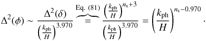$Δ^{2} (φ) ~ \frac{Δ^{2} (δ)}{{(\frac{k_{ph}}{H})}^{3.970}} \overset{Eq . (81)}{\overset{􏽺 0 􏽽􏽼 0 􏽻}{=}} \frac{{(\frac{k_{ph}}{H})}^{n_{s} + 3}}{{(\frac{k_{ph}}{H})}^{3.970}} = {(\frac{k_{ph}}{H})}^{n_{s} - 0.970} \cdot$ $\begin{equation} \Dl^2 (\phi) \sim \frac{\Dl^2 (\dl)}{\left ( \frac{k_{\rm ph}}{H} \right )^{3.970}} \overbrace{=}^{\rm Eq.~(81)} \frac{\left ( \frac{k_{\rm ph}}{H} \right )^{n_{\rm s} + 3}}{\left ( \frac{k_{\rm ph}}{H} \right )^{3.970}} = \left ( \frac{k_{\rm ph}}{H} \right )^{n_{\rm s} - 0.970} \cdot \end{equation}$ (89)When we assume that the power spectrum of metric perturbations is scale invariant, that is, Δ²(φ) ~ k⁰, as implied by CMB anisotropy measurements (see, e.g., Komatsu et al. 2009, 2011) and several other physical arguments (see, e.g., Mukhanov 2005; Padmanabhan 1993; Peacock 1999), Eq. (89) yields $n_{s} = 0.970.$ $\begin{equation} n_{\rm s} = 0.970 . \end{equation}$ (90)The requirement that Δ²(φ) ~ k⁰ implies that in Eqs. (61), (68), and (72), $\hbox{${\cal C}_1 (k) \sim k^{-3/2}$}$ (cf. the combination of Eqs. (60) and (82)), in complete agreement with the (so-called) vacuum assumption, arising from inflationary cosmology amendments (cf. Liddle & Lyth 1993, Eq. (5.34)). In view of Eqs. (83) and (90), we conclude that although in principle there is no reason why the rest-mass density spectrum should exhibit a power-law behavior, in the context of the polytropic DM model under consideration, it effectively does so, that is, $Δ^{2} (δ) ~ k_{ph}^{3 + n_{s}^{eff}}, with n_{s}^{eff} = 0.970.$ $\begin{equation} \Dl^2 (\dl) \sim k_{\rm ph}^{3 + n_{\rm s}^{\rm eff}}, ~\mbox{with} ~~ n_{\rm s}^{\rm eff} = 0.970 . \end{equation}$ (91)We note that the effective scalar spectral index given by Eq. (91) is slightly lower than unity, where the value n_s = 1 corresponds to the Harrison-Zel’dovich-Peebles (scale-invariant) spectrum, for which Δ²(δ) ~ k⁴, that is, | δ | ² ~ k (Harrison 1970; Peebles & Yu 1970; Zel’dovich & Novikov 1970). It is now well established that in realistic cosmology, more power is attributed to large scales, that is, n_s< 1, at 5σ confidence level (see, e.g., Bennet et al. 2013; Li et al. 2013), in complete agreement with amendments that reach as far back as slow-roll inflation (see, e.g., Liddle & Lyth 2000; Springel et al. 2006). In this context, the theoretically derived value (91) for the effective scalar spectral index of rest-mass density perturbations in a polytropic DM model of constant pressure reproduces the corresponding observational Planck result, $n_{s}^{obs} = 0.968 \pm 0.006$ $\hbox{$n_{\rm s}^{\rm obs} = 0.968 \pm 0.006$}$ (Planck Collaboration XIII 2016).

Fig. 7

Plot of Eq. (87), showing small-scale perturbations in the Γ = 0 limit of a polytropic DM model (red solid line). The straight dashed lines represent Eq. (88) for β = 1 (green dashed line) and β = 0.60 (blue dashed line), each one of slope α = 3.970. It is evident that as long as Δ²(φ) ~ k⁰, polytropic perturbations with $(\frac{k_{ph}}{H}) \geq 5$ $\hbox{$\left ( \frac{k_{\rm ph}}{H} \right ) \geq 5$}$ exhibit an effective power-law behavior with a scalar spectral index equal to $n_{s}^{eff} = 0.970$ $\hbox{$n_{\rm s}^{\rm eff} = 0.970$}$ .

To summarize, matter perturbations of linear dimensions smaller than the Hubble radius at any t, when considered in the ΛCDM-like (i.e., Γ = 0) limit of a polytropic DM model, effectively exhibit a power-law behavior of the form $| δ |^{2} ~ k^{n_{s}^{eff}}$ $\hbox{$\vert \dl \vert^2 \sim k^{n_{\rm s}^{\rm eff}}$}$ , with the associated scalar spectral index being equal to $n_{s}^{eff} = 0.970$ $\hbox{$n_{\rm s}^{\rm eff} = 0.970$}$ . To the best of our knowledge, this is the first time that a conventional model with practically no free parameters predicts a theoretical result so close to observation.

6. Discussion

In the unified DM framework, Kleidis & Spyrou (2015) proposed that the constituents of the cosmological dark sector (i.e., DM and DE) can (indeed) be treated as a single component when accommodated in the context of a polytropic DM fluid with thermodynamical content. In this model, macroscopically, the DE simply represents the thermodynamic energy of internal motions of the polytropic DM fluid. Depending on only one free parameter, − 0.103 < Γ ≤ 0, the unified DM model under consideration reproduces the distance measurements performed with the aid of the SNe Ia standard candles to high accuracy, avoids the age problem, and significantly alleviates the coincidence problem (see, e.g., Kleidis & Spyrou 2016). Furthermore, in its Γ = 0 (ΛCDM-like) limit, this model fully compromises the currently admitted behavior of the total EoS parameter in terms of z (cf. Fig. 1). We here demonstrated that in its ΛCDM-like limit, the polytropic DM model under consideration is also compatible with current observational data concerning structure formation. To do so, we explored the evolution of cosmological perturbations in the Γ = 0(p = const. ≠ 0) limit of the aforementioned unified DM model.

In this case, the differential equations that govern the evolution of cosmological perturbations decouple, so that for z ≥ 100, when the DM structures had already been formed (see, e.g., Sandvik et al. 2004; Naoz & Barkana 2005; Knobel 2012), they can be solved analytically. Accordingly, in the Newtonian gauge, we obtained the form of the generalized Newtonian potential, φ, of the rest-mass density contrast, δ, and of the comoving peculiar velocity field, υ, as functions of the cosmological redshift, z. An analysis of these results showed that our solution for { φ,δ } reproduces every main effect previously known from conventional (i.e., pressureless CDM) cosmological perturbation theory, while the non-zero polytropic pressure drives the evolution of peculiar velocities along the lines of the rms-velocity law of conventional statistical physics.

In particular, for z ≥ 100, the generalized Newtonian potential is | φ | ≈ const. (cf. Fig. 2), justifying the current scientific perception that in the vicinity of the matter-dominated era, metric perturbations were (more or less) constant (see, e.g., Knobel 2012). On the other hand, for matter perturbations, small-scale modes (i.e., those lying well within the horizon) conform to high accuracy (cf. Fig. 4) with the Meszaros effect (Meszaros 1974), while those of linear dimensions comparable to the present-time value of the Hubble radius are suppressed (cf. Fig. 3) as ${(1 + z^{)}}^{-1}$ $\hbox{$\left ( 1 + z \right )^{-1}$}$ (cf. Eq. (69)). In other words, in the early matter-dominated era (100 ≤ z ≤ 1090), only the small-scale structures we see today were allowed to be formed, which must have subsequently aggregated to form larger structures later (at lower values of cosmological redshift), in compatibility with the CDM approach (Bond & Szalay 1983). Finally, for z ≥ 11, the non-zero polytropic pressure results in the modification of the functional dependence of ⟨ υ_pec ⟩ over R, which, on the approach to the present epoch, is no longer redshifted away, as predicted by conventional (i.e., pressureless) structure formation theory (see, e.g., Peacock 1999; Sparke & Ghallagher 2007), but instead, it increases (cf. Fig. 5) in agreement with the rms-velocity law of statistical physics (cf. Eqs. (13) and (14)). This result could provide a convenient tool for either conceding or rejecting the polytropic DM model under consideration, for example, by the forthcoming Euclid mission².

We also examined the dimensionless power spectrum of rest-mass density perturbations in the Γ = 0 (ΛCDM-like) limit of the unified DM model. In this case, provided that the corresponding spectrum of metric perturbations is scale invariant, as implied by CMB anisotropy measurements (see, e.g., Komatsu et al. 2009, 2011) and several other physical arguments (see, e.g., Padmanabhan 1993; Peacock 1999), the polytropic DM model with Γ = 0 is equivalent to a cosmological model in which the matter perturbation spectrum effectively exhibits a power-law dependence on the (physical) wavenumber, of the form $| δ |^{2} ~ k^{n_{s}^{eff}}$ $\hbox{$\vert \dl \vert^2 \sim k^{n_{\rm s}^{\rm eff}}$}$ , with the associated scalar spectral index being equal to $n_{s}^{eff} = 0.970$ $\hbox{$n_{\rm s}^{\rm eff} = 0.970$}$ (cf. Fig. 7). It is worth noting that this value differes only slightly from the corresponding observational Planck result (Planck Collaboration XIII 2016), that is, $n_{s}^{obs} = 0.968 \pm 0.006$ $\hbox{$n_{\rm s}^{\rm obs} = 0.968 \pm 0.006$}$ . To the best of our knowledge, this is the first time that a conventional model with practically no free parameters theoretically reproduces a previously observed result.

¹

See, e.g., http://sci.esa.int/euclid

²

See http://sci.esa.int/euclid

Acknowledgments

The authors would like to thank the anonymous referee for the critical comments and useful suggestions that greatly improved the final form of the article. Financial support by the Research Committee of the Technological Education Institute of Central Macedonia at Serres, Greece, under grant SAT/ME/141216-279/11, is gratefully acknowledged.

References

Adriani, O., Barbarino, G. C., Bazilevskaya, G. A., et al. (PAMELA Collaboration) 2009, Nature, 458, 607 [CrossRef] [PubMed] [Google Scholar]
Adriani, O., Barbarino, G. C., Bazilevskaya, G. A., et al. (PAMELA Collaboration) 2010, Phys. Rev. Lett., 105, 121101 [NASA ADS] [CrossRef] [PubMed] [Google Scholar]
Aguilar, M., Ali Cavasonza, L., Ambrosi, G., et al. (AMS Collaboration) 2016, Phys. Rev. Lett., 117, 231102 [NASA ADS] [CrossRef] [Google Scholar]
Albert, A., Anderson, B., Bechtol, K., et al. (The Fermi LAT; DES Collaborations) 2017, ApJ, 834, 110 [NASA ADS] [CrossRef] [Google Scholar]
Allen, S. W., Schmidt, R. W., Ebeling, H., Fabian, A. C., & van Speybroeck, L. 2004, MNRAS, 353, 457 [NASA ADS] [CrossRef] [Google Scholar]
Amanullah, R., Stanishev, V., Goobar, A., et al. (Supernova Cosmology Project Group) 2008, A&A, 486, 375 [NASA ADS] [CrossRef] [EDP Sciences] [Google Scholar]
Amanullah, R., Lidman, C., Rubin, D., et al. (Supernova Cosmology Project Group) 2010, ApJ, 716, 712 [NASA ADS] [CrossRef] [Google Scholar]
Amendola, L., Appleby, S., Bacon, S., et al. (The Euclid Theory Working Group) 2013, Liv. Rev. Rel., 16, 6 [Google Scholar]
Arkani-Hamed, N., Finkbeiner, D. P., Slatyer, T. R., & Weiner, N. 2009, Phys. Rev. D, 79, 015014 [NASA ADS] [CrossRef] [Google Scholar]
Armendariz-Picon, C., Mukhanov, V. F., & Steinhardt, P. J. 2001, Phys. Rev. D, 63, 103510 [NASA ADS] [CrossRef] [MathSciNet] [Google Scholar]
Asadzadeh, S., Safari, Z., Karami, K., & Abdolmaleki, A. 2014, Int. J. Theor. Phys., 53, 1248 [CrossRef] [Google Scholar]
Astier, P., Guy, J., Regnault, N., et al. (SNLS Collaboration) 2006, A&A, 447, 31 [NASA ADS] [CrossRef] [EDP Sciences] [Google Scholar]
Balakin, A. B., Pavón, D., Schwarz, D. J., & Zimdahl, W. 2003, New J. Phys., 5, 85 [NASA ADS] [CrossRef] [Google Scholar]
Bardeen, J. M. 1980, Phys. Rev. D, 22, 1882 [NASA ADS] [CrossRef] [MathSciNet] [Google Scholar]
Barris, B., Tonry, J. L., Blondin, S., et al. (Institute for Astronomy Deep Survey) 2004, ApJ, 602, 571 [NASA ADS] [CrossRef] [Google Scholar]
Basilakos, S., & Plionis, M. 2009, A&A, 507, 47 [NASA ADS] [CrossRef] [EDP Sciences] [Google Scholar]
Basilakos, S., & Plionis, M. 2010, in Invisible Universe: Conference Proceedings, AIP Conf. Proc., 1241, 721 [NASA ADS] [CrossRef] [Google Scholar]
Bean, R., & Doré, O. 2003, Phys. Rev. D, 68, 023515 [NASA ADS] [CrossRef] [Google Scholar]
Bennett, C. L., Larson, D., Weiland, J. L., et al. (WMAP Collaboration) 2013, ApJS, 208, 20 [Google Scholar]
Bento, M. C., Bertolami, O., & Sen, A. A. 2002, Phys. Rev. D, 66, 043507 [NASA ADS] [CrossRef] [MathSciNet] [Google Scholar]
Bharadwaj, S., & Kar, S. 2003, Phys. Rev. D, 68, 023516 [NASA ADS] [CrossRef] [Google Scholar]
Bilić, N., Tupper, G. B., & Viollier, R. D. 2002, Phys. Lett. B, 535, 17 [NASA ADS] [CrossRef] [Google Scholar]
Böhmer, C. G., & Harko, T. 2007, J. Cosmol. Astropart. Phys., 6, 25 [Google Scholar]
Bond, J. R., & Szalay, A. S. 1983, ApJ, 274, 443 [Google Scholar]
Bond, J. R., Efstathiou G., & Silk, J. 1980, Phys. Lett., 45, 1980 [NASA ADS] [CrossRef] [Google Scholar]
Boughn, S., & Crittenden, R. 2004, Nature, 427, 45 [NASA ADS] [CrossRef] [EDP Sciences] [PubMed] [Google Scholar]
Bousso, R., & Polchinski, J. 2000, J. Height Energy Phys., 06, 006 [Google Scholar]
Capozziello, S., Carloni, S., & Troisi, A. 2003, Recent Res. Dev. Astron. Astrophys., 1, 625 [Google Scholar]
Capozziello, S., Luongo, O., & Saridakis, E. N. 2015, Phys. Rev. D, 91, 124037 [NASA ADS] [CrossRef] [Google Scholar]
Caldwell, R. R. 2002, Phys. Lett. B, 545, 23 [NASA ADS] [CrossRef] [Google Scholar]
Caldwell, R. R., & Kamionkowski, M. 2009, Ann. Rev. Nucl. Part. Sci., 59, 397 [NASA ADS] [CrossRef] [Google Scholar]
Caldwell, R. R., Dave, R., & Steinhardt, P. J. 1998, Phys. Rev. Lett., 80, 1528 [NASA ADS] [CrossRef] [Google Scholar]
Chandrasekhar, S. 1939, An Introduction to the Study of Stellar Structure (Chicago University Press) [Google Scholar]
Chavanis, P.-H. 2012, ArXiv e-prints [arXiv:1208.1192] [Google Scholar]
Chavanis, P.-H. 2014a, EPJ Plus, 129, 38 [NASA ADS] [EDP Sciences] [Google Scholar]
Chavanis, P.-H. 2014b, EPJ Plus, 129, 222 [EDP Sciences] [Google Scholar]
Cirelli, M., Kadastik, M., Raidal, M., & Strumia, A. 2009, Nucl. Phys. B, 813, 1 [NASA ADS] [CrossRef] [Google Scholar]
Cohen, T., & Zurek, K. 2010, Phys. Rev. Lett., 104, 101301 [NASA ADS] [CrossRef] [PubMed] [Google Scholar]
Cohen, A. G., Kaplan, D. M., & Nelson, A. G. 1999, Phys. Rev. Lett., 82, 4971 [NASA ADS] [CrossRef] [MathSciNet] [Google Scholar]
Contreras, C., Hamuy, M., Phillips, M. M., et al. (The Carnegie SN Project) 2010, AJ, 139, 519 [NASA ADS] [CrossRef] [Google Scholar]
Copeland, E. J., Sami, M., & Tsujikawa, S. 2006, Int. J. Mod. Phys. D, 15, 1753 [NASA ADS] [CrossRef] [MathSciNet] [Google Scholar]
Deffayet, C., Dvali, G., & Gabadadze, G. 2002, Phys. Rev. D, 65, 044023 [NASA ADS] [CrossRef] [MathSciNet] [Google Scholar]
Dutta, S., & Scherrer, R. J. 2010, Phys. Rev. D, 82, 043526 [NASA ADS] [CrossRef] [Google Scholar]
Dvali, G. R., Gabadadze, G., & Porratti, M. 2000, Phys. Lett. B, 485, 208 [NASA ADS] [CrossRef] [MathSciNet] [Google Scholar]
Eisenstein, D. J., Zehavi, I., Hogg, D. W., et al. (SDSS Collaboration) 2005, ApJ, 633, 560 [NASA ADS] [CrossRef] [Google Scholar]
Esposito-Farese, G., & Polarski, D. 2001, Phys. Rev. D, 63, 063504 [NASA ADS] [CrossRef] [Google Scholar]
Fardon, R., Nelson, A. E., & Weiner, N. 2004, J. Cosmol. Astropart. Phys., 10, 005 [Google Scholar]
Fock, V. 1959, The Theory of Space, Time and Gravitation (London: Pergamon Press) [Google Scholar]
Freese, K. 2005, New Astron. Rev., 49, 103 [NASA ADS] [CrossRef] [Google Scholar]
Freese, K., & Lewis, M. 2002, Phys. Lett. B, 540, 1 [NASA ADS] [CrossRef] [MathSciNet] [Google Scholar]
Frieman, J. A., Turner, M. S., & Huterer, D. 2008, ARA&A, 46, 385 2002 [NASA ADS] [CrossRef] [Google Scholar]
Garnavich, P. M., Jha, S., Challis, P., et al. (High-z Supernova Search Team) 1998, ApJ, 509, 74 [NASA ADS] [CrossRef] [Google Scholar]
Giostri, R., Vargas dos Santos, M., Waga, I., et al. 2012, J. Cosmol. Astropart. Phys., 03, 027 [NASA ADS] [CrossRef] [Google Scholar]
Gradshteyn, I. S., & Ryzhik, I. M. 2007, Tables of Integrals, Series and Products 7th edn. (Amsterdam: Elsevier – Academic Press) [Google Scholar]
Gondolo, P., & Freese, K. 2003, Phys. Rev. D, 68, 063509 [NASA ADS] [CrossRef] [Google Scholar]
Guy, J., Sullivan, M., Conley, A., et al. (SNLS Collaboration) 2010, A&A, 466, A11 [Google Scholar]
Hamuy, M., Phillips, M. M., Suntzeff, N. B., et al. 1996, AJ, 112, 2408 [NASA ADS] [CrossRef] [Google Scholar]
Harrison, E. R. 1970, Phys. Rev. D, 1, 2726 [NASA ADS] [CrossRef] [Google Scholar]
Hawking, S. 1966, ApJ, 145, 544 [NASA ADS] [CrossRef] [Google Scholar]
Hicken, M., Challis, P., Jha, S., et al. 2009a, ApJ, 700, 331 [NASA ADS] [CrossRef] [Google Scholar]
Hicken, M., Wood-Vasey, M., Blondin, S., et al. 2009b, ApJ, 700, 1097 [NASA ADS] [CrossRef] [Google Scholar]
Holtzman, J. A., Marriner, J., Kessler, R., et al. (SDSS-II Collaboration) 2008, AJ, 136, 2306 [NASA ADS] [CrossRef] [Google Scholar]
Hooper, D., Finkbeiner, D. P., & Dobler, G. 2007, Phys. Rev. D, 76, 083012 [NASA ADS] [CrossRef] [Google Scholar]
Horedt, G. P. 2004, Polytropes: Applications in Astrophysics and Related Fields (Dordrecht: Kluwer Academic Publishers) [Google Scholar]
Horvath, I., Hakkila, J., & Bagoly, Z. 2013, in GRB 2013: 7th Huntsville Gamma-Ray Burst Symposium, eConf Proc.C1304143, 33 [Google Scholar]
Huterer, D. 2002, Phys. Rev. D, 65, 063001 [NASA ADS] [CrossRef] [Google Scholar]
Jha, S., Kirshner, R. P., Challis, P., et al. (ESSENCE Supernova Survey Team) 2006, AJ, 131, 527 [NASA ADS] [CrossRef] [Google Scholar]
Kamenshchik, A., Moschella, U., & Pasquier, V. 2001, Phys. Lett. B, 487, 7 [NASA ADS] [Google Scholar]
Karami, K., & Abdolmaleki, A. 2010a, Astrophys. Space Sci., 330, 139 [NASA ADS] [CrossRef] [Google Scholar]
Karami, K., & Abdolmaleki, A. 2010b, Phys. Scr., 81, 055901 [NASA ADS] [CrossRef] [Google Scholar]
Karami, K., & Abdolmaleki, A. 2012, J. Phys. Conf. Ser., 375, 032009 [NASA ADS] [CrossRef] [Google Scholar]
Karami, K., & Khaledian, M. S. 2012, Int. J. Mod. Phys. D, 21, 1250083 [NASA ADS] [CrossRef] [Google Scholar]
Karami, K., Ghaffari, S., & Fehri, J. 2009, Eur. Phys. J. C, 64, 85 [NASA ADS] [CrossRef] [EDP Sciences] [Google Scholar]
Kessler, R., Becker, A. C., Cinabro, D., et al. (SDSS-II Collaboration) 2009, ApJS, 185, 32 [NASA ADS] [CrossRef] [Google Scholar]
Kleidis, K., & Spyrou, N. K. 2015, A&A, 576, A23 [NASA ADS] [CrossRef] [EDP Sciences] [Google Scholar]
Kleidis, K., & Spyrou, N. K. 2016, Entropy, 18, 094 [NASA ADS] [CrossRef] [Google Scholar]
Klypin, A., Holtzman, J., Primack, J. R., & Regos, E. 1993, ApJ, 416, 1 [NASA ADS] [CrossRef] [Google Scholar]
Knobel, C. 2012, ArXiv e-prints [arXiv:1208.5931] [Google Scholar]
Knop, R. A., Aldering, G., Amanullah, R., et al. (Supernova Cosmology Project Group) 2003, ApJ, 598, 102 [NASA ADS] [CrossRef] [Google Scholar]
Kodama, H., & Sasaki, M. 1984, Prog. Theor. Phys. Suppl., 78, 1 [NASA ADS] [CrossRef] [Google Scholar]
Komatsu, E., Dunkley, J., Nolta, M.R., et al. (WMAP Collaboration) 2009, ApJS, 180, 330 [NASA ADS] [CrossRef] [Google Scholar]
Komatsu, E., Smith, K. M., Dunkley, J., et al. (WMAP Collaboration) 2011, ApJS, 192, 18 [NASA ADS] [CrossRef] [Google Scholar]
Koutsoumbas, G., Ntrekis, K., Papantonopoulos, E., & Saridakis, E. 2017, ArXiv e-prints [arXiv:1704.08640] [Google Scholar]
Kowalski, M., Rubin, D., Aldering, G., et al. (Supernova Cosmology Project Group) 2008, ApJ, 686, 749 [NASA ADS] [CrossRef] [Google Scholar]
Krisciunas, K., Garnavich, P. M., Challis, P., et al. (ESSENCE SN Survey Team) 2005, AJ, 130, 2472 [Google Scholar]
Landau, L. D., & Lifshitz, E. M. 1969, Statistical Physics (Oxford: Pergamon Press) [Google Scholar]
Li, M. 2004, Phys. Lett. B, 603, 1 [NASA ADS] [CrossRef] [Google Scholar]
Li, H., Xia, J.-Q., & Zhang, X. 2013, Physics of the Dark Universe, 2, 188 [NASA ADS] [CrossRef] [Google Scholar]
Liddle, A. R., & Lyth, D. H. 1993, Phys. Rep., 231, 1 [NASA ADS] [CrossRef] [Google Scholar]
Liddle, A. R., & Lyth, D. H. 2000, Cosmological Inflation and Large-Scale Structure (Cambridge: Cambridge University Press) [Google Scholar]
Lifshitz, E. M. 1946, J. Phys. USSR, 10, 116 [Google Scholar]
Lifshitz, E. M., & Khalatnikov, I. M. 1963, Adv. Phys., 12, 185 [NASA ADS] [CrossRef] [MathSciNet] [Google Scholar]
Lima, J. A. S., Silva, F. E., & Santos, R. C. 2008, Class. Quant. Grav., 25, 205006 [NASA ADS] [CrossRef] [Google Scholar]
Lima, J. A. S., Jesus, J. F., & Oliveira, F. A. 2010, J. Cosmol. Astropart. Phys., 11, 027 [NASA ADS] [CrossRef] [Google Scholar]
Lima, J. A. S., Basilakos, S., & Costa, F. E. M. 2012, Phys. Rev. D, 86, 103534 [NASA ADS] [CrossRef] [Google Scholar]
Linde, A. 1990, Particle Physics and Inflationary Cosmology (Chur, Switzerland: Harwood) [Google Scholar]
Linder, E. V., & Jenkins, A. 2003, MNRAS, 346, 573 [NASA ADS] [CrossRef] [Google Scholar]
Ma, C. P., & Bertschinger, E. 1995, ApJ, 455, 7 [NASA ADS] [CrossRef] [Google Scholar]
Makler, M., de Olivera, S. Q., & Waga, I. et al. 2003, Phys. Lett. B, 555, 1 [NASA ADS] [CrossRef] [Google Scholar]
Malekjani, M., Khodam-Mohamadi, A., & Taji, M. 2011, Int. J. Theor. Phys., 50, 3112 [CrossRef] [Google Scholar]
Meszaros, P. 1974, A&A, 37, 225 [NASA ADS] [Google Scholar]
Miao, L. I., Xiao-Dong, L. I., Wang, S., & Wang, Y. 2011, Commun. Theor. Phys., 56, 525 [NASA ADS] [CrossRef] [Google Scholar]
Miknaitis, G., Pignata, G., Rest, A., et al. (ESSENCE Supernova Survey Team) 2007, ApJ, 666, 674 [NASA ADS] [CrossRef] [Google Scholar]
Mongan, T. R. 2001, Gen. Rel.. Grav., 33, 1415 [NASA ADS] [CrossRef] [Google Scholar]
Mukhanov, V. F. 2005, Physical Foundations of Cosmology (Cambridge: Cambridge University Press) [Google Scholar]
Mukhanov, V. F., Feldman, H. A., & Brandenberger, R. H. 1992, Phys. Rep., 215, 203 [NASA ADS] [CrossRef] [MathSciNet] [Google Scholar]
Mukhopadhyay, V., Ray, S., & Dutta, C. S. 2008, Mod. Phys. Lett. A, 23, 3187 [NASA ADS] [CrossRef] [Google Scholar]
Naoz, S., & Barkana, R. 2005, MNRAS, 362, 1047 [NASA ADS] [CrossRef] [Google Scholar]
Nojiri, S., & Odintsov, S. D. 2007, Int. J. Geom. Meth. Mod. Phys., 04, 115 [Google Scholar]
Nojiri, S., Odintsov, S. D., & Tsujikawa, S. 2005, Phys. Rev. D, 71, 063004 [NASA ADS] [CrossRef] [Google Scholar]
Nunez, D., Sussman, R. A., Zavala, J., Cabral-Rosetti, L. G., & Matos, T. 2006, in AIP Conf. Proc. 857, eds. A. Bashir, V. Villanueva, L. Villasenor, M. A. Perez, & L. Urrutia, 316 [Google Scholar]
Olive, K. A., Agashe, K., Amsler, C., et al. (Particle Data Group) 2014, Chin. Phys. C, 38, 090001 [NASA ADS] [CrossRef] [MathSciNet] [Google Scholar]
Olver, F. W. J., Lozier, D. W., Boisvert, R. F., & Clark, C. W. 2010, NIST Handbook of Mathematical Functions (New York: Cambridge University Press) [Google Scholar]
Padmanabhan, T. 1993, Structure Formation in the Universe (Cambridge: Cambridge University Press) [Google Scholar]
Padmanabhan, T. 2002, Phys. Rev. D, 66, 021301 [NASA ADS] [CrossRef] [MathSciNet] [Google Scholar]
Padmanabhan, T. 2003, Phys. Rep., 380, 235 [NASA ADS] [CrossRef] [MathSciNet] [Google Scholar]
Pavón, D., & Zimdahl, W. 2005, Phys. Lett. B, 628, 206 [NASA ADS] [CrossRef] [Google Scholar]
Peacock, J. A. 1999, Cosmological Physics (Cambridge: Cambridge University Press) [Google Scholar]
Peccei, R. D. 2005, Phys. Rev. D, 71, 023527 [NASA ADS] [CrossRef] [Google Scholar]
Peebles, P. J. E., & Yu, J. T. 1970, ApJ, 162, 815 [NASA ADS] [CrossRef] [Google Scholar]
Peebles, P. J. E. 1980, The Large Scale Structure of the Universe (Princeton: Princeton University Press) [Google Scholar]
Percival, W. J., Reid, B. A., Eisenstein, D. J., et al. (SDSS Collaboration) 2010, MNRAS, 401, 2148 [NASA ADS] [CrossRef] [Google Scholar]
Perivolaropoulos, L. 2003, Phys. Rev. D, 67, 123516 [NASA ADS] [CrossRef] [MathSciNet] [Google Scholar]
Perlmutter, S., Aldering, G., Valle, M. D., et al. (Supernova Cosmology Project Group) 1998, Nature, 391, 51 [CrossRef] [Google Scholar]
Perlmutter, S., Aldering, G., Goldhaber, G., et al. (Supernova Cosmology Project Group) 1999a, ApJ, 517, 565 [NASA ADS] [CrossRef] [Google Scholar]
Perlmutter, S., Turner, M. S., & White, M. 1999b, Phys. Rev. Lett., 83, 670 [NASA ADS] [CrossRef] [Google Scholar]
Planck Collaboration XIII. 2016, A&A, 594, A13 [NASA ADS] [CrossRef] [EDP Sciences] [Google Scholar]
Ren, J., & Meng, X. H. 2006, Phys. Lett. B, 633, 1 [NASA ADS] [CrossRef] [Google Scholar]
Riess, A. G., Filippenko, A. V., Challis, P., et al. (High-z Supernova Search Team) 1998, AJ, 116, 1009 [NASA ADS] [CrossRef] [Google Scholar]
Riess, A. G., Nugent, P. E., Gilliland, R. L., et al. (High-z Supernova Search Team) 2001, ApJ, 560, 49 [NASA ADS] [CrossRef] [Google Scholar]
Riess, A. G., Strolger, L.-G., Tonry, J., et al. (High-z Supernova Search Team) 2004, ApJ, 607, 665 [NASA ADS] [CrossRef] [Google Scholar]
Riess, A. G., Strolger, L.-G., Casertano, S., et al. (High-z Supernova Search Team) 2007, ApJ, 659, 98 [NASA ADS] [CrossRef] [Google Scholar]
Sachs, K., & Wolfe, A. M. 1967, ApJ, 147, 73 [NASA ADS] [CrossRef] [Google Scholar]
Sahni, V., & Starobinsky, A. 2000, Int. J. Mod. Phys. D, 9, 373 [Google Scholar]
Sami, M., Savchenko, N., & Toporensky, A. 2004, Phys. Rev. D, 70, 123528 [NASA ADS] [CrossRef] [Google Scholar]
Sandvik, H. B., Tegmark, M., Zaldarriaga, M., & Waga, I. 2004, Phys. Rev. D, 69, 123524 [NASA ADS] [CrossRef] [Google Scholar]
Saxton, C. J., & Ferreras, I. 2010, MNRAS, 405, 77 [NASA ADS] [Google Scholar]
Saxton, C. J., & Wu, K. 2008, MNRAS, 391, 1403 [NASA ADS] [CrossRef] [Google Scholar]
Saxton, C. J., Younsi, Z., & Wu, K. 2016, MNRAS, 461, 4295 [NASA ADS] [CrossRef] [Google Scholar]
Scherrer, R. J. 2004, Phys. Rev. Lett., 93, 011301 [NASA ADS] [CrossRef] [Google Scholar]
Schmidt, B. P., Suntzeff, N. B., Phillips, M. M., et al. (High-z Supernova Search Team) 1998, ApJ, 507, 46 [NASA ADS] [CrossRef] [Google Scholar]
Seljak, U., Slosar, A., & McDonald, P. 2006, J. Cosmol. Astropart. Phys., 0610, 014 [Google Scholar]
Sen, A. A., & Scherrer, R. J. 2005, Phys. Rev. D, 72, 063511 [NASA ADS] [CrossRef] [Google Scholar]
Spergel, D. N., & Steinhardt, P. J. 2000, Phys. Rev. Lett., 84, 3760 [NASA ADS] [CrossRef] [PubMed] [Google Scholar]
Springel, V., Frenk, C. S., & White, S. D. M. 2006, Nature, 440, 1137 [NASA ADS] [CrossRef] [PubMed] [Google Scholar]
Stefancić, H. 2005, Phys. Rev. D, 71, 084024 [NASA ADS] [CrossRef] [MathSciNet] [Google Scholar]
Su, K.-Y., & Chen, P. 2009, Phys. Rev. D, 79, 128301 [NASA ADS] [CrossRef] [Google Scholar]
Suzuki, N., Rubin, D., Lidman, C., et al. (Supernova Cosmology Project Group) 2012, ApJ, 746, 85 [NASA ADS] [CrossRef] [Google Scholar]
Tonry, J. L., Schmidt, B. P., Barris, B., et al. (High-z Supernova Search Team) 2003, ApJ, 594, 1 [NASA ADS] [CrossRef] [Google Scholar]
Turner, M. S., & White, M. 1997, Phys. Rev. D, 56, 4439 [NASA ADS] [CrossRef] [Google Scholar]
Van den Aarssen, L., Bringmann, T., & Pfommer, C. 2012, Phys. Rev. Lett., 109, 231301 [NASA ADS] [CrossRef] [Google Scholar]
Veeraraghavan, S., & Stebbins, A. 1990, ApJ, 365, 37 [NASA ADS] [CrossRef] [Google Scholar]
Wang, Y., Freese, K., Gondolo, P., & Lewis, M. 2003, ApJ, 594, 25 [NASA ADS] [CrossRef] [Google Scholar]
Weinberg, S. 1972, Gravitation and Cosmology (New York: John Wiley & Sons Inc.) [Google Scholar]
Wood-Vasey, W. M., Miknaitis, G., Stubbs, C. W., et al. (ESSENCE Supernova Survey Team) 2007, ApJ, 666, 694 [NASA ADS] [CrossRef] [Google Scholar]
Xu, L., Wang, Y., & Noh, H. 2012, Phys. Rev. D, 85, 043003 [NASA ADS] [CrossRef] [Google Scholar]
Zavala, J., Nunez, D., Sussman, R. A., Cabral-Rosetti, L. G., & Matos, T. 2006, J. Cosmol. Astropart. Phys., 6, 8 [Google Scholar]
Zel’dovich, Ya. B., & Novikov, I. D. 1970, Astrofizika, 6, 379 [NASA ADS] [Google Scholar]
Zimdahl, W., Schwarz, D. J., Balakin, A. B., & Pavón, D. 2001, Phys. Rev. D, 64, 3501 [NASA ADS] [CrossRef] [MathSciNet] [Google Scholar]

All Figures

	Fig. 1 Total EoS parameter, w_tot, as a function of the cosmological redshift, z, in the context of the ΛCDM-like (i.e., Γ = 0) limit of the polytropic DM model. We note that today, w_tot ≈ − 0.7, while for z ≥ 3, it remains very close to zero, as suggested by ΛCDM cosmology.
In the text

	Fig. 2 Amplitude of the generalized Newtonian potential, \| φ \|, normalized over $\hbox{$\vert {\cal C}_1 (k) \vert$}$ , as a function of w = 1 + z. It is evident that for w ≥ 100, \| φ \| = const. to high accuracy.
In the text

Fig. 3

Amplitude of the rest-mass density contrast, | δ |, normalized over $\hbox{$\vert {\cal C}_1 (k) \vert$}$ , as a function of the Universe scale factor, R, for $(\frac{k_{0}^{ph}}{H_{0}}) = 10$ $\hbox{$\left( \frac{k_0^{\rm ph}}{H_0} \right) = 10$}$ (blue solid line), and 100 (red solid line). The vertical dashed line marks the recombination epoch. We observe that the longer the present timescale of a structure, the more suppressed the associated perturbation mode.

In the text

Fig. 4

Amplitude of the rest-mass density contrast, | δ |, in units of $\hbox{$\vert {\cal C}_1 (k) \vert$}$ , as a function of the Universe scale factor, R, for $(\frac{k_{0}^{ph}}{H_{0}}) = 10$ $\hbox{$\left( \frac{k_0^{\rm ph}}{H_0} \right) = 10$}$ (blue solid line), 100 (red solid line), and 1000 (green solid line). The vertical dashed line marks the onset of matter-dominated era, in which our (linear) perturbative analysis holds. We observe that for z< 1090, polytropic DM perturbations conform with the Meszaros effect (i.e., δ ~ R) to high accuracy.

In the text

Fig. 5

Average peculiar velocity field, ⟨ υ_pec ⟩, normalized over $\hbox{$\langle k {\cal C}_1 (k) \rangle$}$ , as a function of the Universe scale factor, R, for $(\frac{k_{0}^{ph}}{H_{0}}) = 100$ $\hbox{$\left( \frac{k_0^{\rm ph}}{H_0} \right) = 100$}$ (red solid line) and 1000 (green solid line). We observe that within the linear regime, peculiar velocities conform with the rms-velocity law of statistical physics (i.e., $⟨ υ ⟩ ~ \sqrt{R}$ $\hbox{$\langle \ups \rangle \sim \sqrt{R}$}$ ) given by Eq. (14). In both curves, the receding part arising for $\frac{R}{R_{0}} \geq 0.2$ $\hbox{$\frac{R}{R_0} \geq 0.2$}$ (z ≤ 4) signals the onset of deviations from the rms-velocity law due to the collapse of linear approximation and Hubble drag.

In the text

	Fig. 6 Equation of motion (79), monitored over the time span corresponding to 50 ≤ w = 1 + z ≤ 1100. It is evident that for w ≥ 100, this constraint is valid to an accuracy higher than 1:10⁷.
In the text

Fig. 7

Plot of Eq. (87), showing small-scale perturbations in the Γ = 0 limit of a polytropic DM model (red solid line). The straight dashed lines represent Eq. (88) for β = 1 (green dashed line) and β = 0.60 (blue dashed line), each one of slope α = 3.970. It is evident that as long as Δ²(φ) ~ k⁰, polytropic perturbations with $(\frac{k_{ph}}{H}) \geq 5$ $\hbox{$\left ( \frac{k_{\rm ph}}{H} \right ) \geq 5$}$ exhibit an effective power-law behavior with a scalar spectral index equal to $n_{s}^{eff} = 0.970$ $\hbox{$n_{\rm s}^{\rm eff} = 0.970$}$ .

In the text

Current usage metrics show cumulative count of Article Views (full-text article views including HTML views, PDF and ePub downloads, according to the available data) and Abstracts Views on Vision4Press platform.

Data correspond to usage on the plateform after 2015. The current usage metrics is available 48-96 hours after online publication and is updated daily on week days.

Initial download of the metrics may take a while.

[1] Adriani, O., Barbarino, G. C., Bazilevskaya, G. A., et al. (PAMELA Collaboration) 2009, Nature, 458, 607 [CrossRef] [PubMed] [Google Scholar]

[2] Adriani, O., Barbarino, G. C., Bazilevskaya, G. A., et al. (PAMELA Collaboration) 2010, Phys. Rev. Lett., 105, 121101 [NASA ADS] [CrossRef] [PubMed] [Google Scholar]

[3] Aguilar, M., Ali Cavasonza, L., Ambrosi, G., et al. (AMS Collaboration) 2016, Phys. Rev. Lett., 117, 231102 [NASA ADS] [CrossRef] [Google Scholar]

[4] Albert, A., Anderson, B., Bechtol, K., et al. (The Fermi LAT; DES Collaborations) 2017, ApJ, 834, 110 [NASA ADS] [CrossRef] [Google Scholar]

[5] Allen, S. W., Schmidt, R. W., Ebeling, H., Fabian, A. C., & van Speybroeck, L. 2004, MNRAS, 353, 457 [NASA ADS] [CrossRef] [Google Scholar]

[6] Amanullah, R., Stanishev, V., Goobar, A., et al. (Supernova Cosmology Project Group) 2008, A&A, 486, 375 [NASA ADS] [CrossRef] [EDP Sciences] [Google Scholar]

[7] Amanullah, R., Lidman, C., Rubin, D., et al. (Supernova Cosmology Project Group) 2010, ApJ, 716, 712 [NASA ADS] [CrossRef] [Google Scholar]

[8] Amendola, L., Appleby, S., Bacon, S., et al. (The Euclid Theory Working Group) 2013, Liv. Rev. Rel., 16, 6 [Google Scholar]

[9] Arkani-Hamed, N., Finkbeiner, D. P., Slatyer, T. R., & Weiner, N. 2009, Phys. Rev. D, 79, 015014 [NASA ADS] [CrossRef] [Google Scholar]

[10] Armendariz-Picon, C., Mukhanov, V. F., & Steinhardt, P. J. 2001, Phys. Rev. D, 63, 103510 [NASA ADS] [CrossRef] [MathSciNet] [Google Scholar]

[11] Asadzadeh, S., Safari, Z., Karami, K., & Abdolmaleki, A. 2014, Int. J. Theor. Phys., 53, 1248 [CrossRef] [Google Scholar]

[12] Astier, P., Guy, J., Regnault, N., et al. (SNLS Collaboration) 2006, A&A, 447, 31 [NASA ADS] [CrossRef] [EDP Sciences] [Google Scholar]

[13] Balakin, A. B., Pavón, D., Schwarz, D. J., & Zimdahl, W. 2003, New J. Phys., 5, 85 [NASA ADS] [CrossRef] [Google Scholar]

[14] Bardeen, J. M. 1980, Phys. Rev. D, 22, 1882 [NASA ADS] [CrossRef] [MathSciNet] [Google Scholar]

[15] Barris, B., Tonry, J. L., Blondin, S., et al. (Institute for Astronomy Deep Survey) 2004, ApJ, 602, 571 [NASA ADS] [CrossRef] [Google Scholar]

[16] Basilakos, S., & Plionis, M. 2009, A&A, 507, 47 [NASA ADS] [CrossRef] [EDP Sciences] [Google Scholar]

[17] Basilakos, S., & Plionis, M. 2010, in Invisible Universe: Conference Proceedings, AIP Conf. Proc., 1241, 721 [NASA ADS] [CrossRef] [Google Scholar]

[18] Bean, R., & Doré, O. 2003, Phys. Rev. D, 68, 023515 [NASA ADS] [CrossRef] [Google Scholar]

[19] Bennett, C. L., Larson, D., Weiland, J. L., et al. (WMAP Collaboration) 2013, ApJS, 208, 20 [Google Scholar]

[20] Bento, M. C., Bertolami, O., & Sen, A. A. 2002, Phys. Rev. D, 66, 043507 [NASA ADS] [CrossRef] [MathSciNet] [Google Scholar]

[21] Bharadwaj, S., & Kar, S. 2003, Phys. Rev. D, 68, 023516 [NASA ADS] [CrossRef] [Google Scholar]

[22] Bilić, N., Tupper, G. B., & Viollier, R. D. 2002, Phys. Lett. B, 535, 17 [NASA ADS] [CrossRef] [Google Scholar]

[23] Böhmer, C. G., & Harko, T. 2007, J. Cosmol. Astropart. Phys., 6, 25 [Google Scholar]

[24] Bond, J. R., & Szalay, A. S. 1983, ApJ, 274, 443 [Google Scholar]

[25] Bond, J. R., Efstathiou G., & Silk, J. 1980, Phys. Lett., 45, 1980 [NASA ADS] [CrossRef] [Google Scholar]

[26] Boughn, S., & Crittenden, R. 2004, Nature, 427, 45 [NASA ADS] [CrossRef] [EDP Sciences] [PubMed] [Google Scholar]

[27] Bousso, R., & Polchinski, J. 2000, J. Height Energy Phys., 06, 006 [Google Scholar]

[28] Capozziello, S., Carloni, S., & Troisi, A. 2003, Recent Res. Dev. Astron. Astrophys., 1, 625 [Google Scholar]

[29] Capozziello, S., Luongo, O., & Saridakis, E. N. 2015, Phys. Rev. D, 91, 124037 [NASA ADS] [CrossRef] [Google Scholar]

[30] Caldwell, R. R. 2002, Phys. Lett. B, 545, 23 [NASA ADS] [CrossRef] [Google Scholar]

[31] Caldwell, R. R., & Kamionkowski, M. 2009, Ann. Rev. Nucl. Part. Sci., 59, 397 [NASA ADS] [CrossRef] [Google Scholar]

[32] Caldwell, R. R., Dave, R., & Steinhardt, P. J. 1998, Phys. Rev. Lett., 80, 1528 [NASA ADS] [CrossRef] [Google Scholar]

[33] Chandrasekhar, S. 1939, An Introduction to the Study of Stellar Structure (Chicago University Press) [Google Scholar]

[34] Chavanis, P.-H. 2012, ArXiv e-prints [arXiv:1208.1192] [Google Scholar]

[35] Chavanis, P.-H. 2014a, EPJ Plus, 129, 38 [NASA ADS] [EDP Sciences] [Google Scholar]

[36] Chavanis, P.-H. 2014b, EPJ Plus, 129, 222 [EDP Sciences] [Google Scholar]

[37] Cirelli, M., Kadastik, M., Raidal, M., & Strumia, A. 2009, Nucl. Phys. B, 813, 1 [NASA ADS] [CrossRef] [Google Scholar]

[38] Cohen, T., & Zurek, K. 2010, Phys. Rev. Lett., 104, 101301 [NASA ADS] [CrossRef] [PubMed] [Google Scholar]

[39] Cohen, A. G., Kaplan, D. M., & Nelson, A. G. 1999, Phys. Rev. Lett., 82, 4971 [NASA ADS] [CrossRef] [MathSciNet] [Google Scholar]

[40] Contreras, C., Hamuy, M., Phillips, M. M., et al. (The Carnegie SN Project) 2010, AJ, 139, 519 [NASA ADS] [CrossRef] [Google Scholar]

[41] Copeland, E. J., Sami, M., & Tsujikawa, S. 2006, Int. J. Mod. Phys. D, 15, 1753 [NASA ADS] [CrossRef] [MathSciNet] [Google Scholar]

[42] Deffayet, C., Dvali, G., & Gabadadze, G. 2002, Phys. Rev. D, 65, 044023 [NASA ADS] [CrossRef] [MathSciNet] [Google Scholar]

[43] Dutta, S., & Scherrer, R. J. 2010, Phys. Rev. D, 82, 043526 [NASA ADS] [CrossRef] [Google Scholar]

[44] Dvali, G. R., Gabadadze, G., & Porratti, M. 2000, Phys. Lett. B, 485, 208 [NASA ADS] [CrossRef] [MathSciNet] [Google Scholar]

[45] Eisenstein, D. J., Zehavi, I., Hogg, D. W., et al. (SDSS Collaboration) 2005, ApJ, 633, 560 [NASA ADS] [CrossRef] [Google Scholar]

[46] Esposito-Farese, G., & Polarski, D. 2001, Phys. Rev. D, 63, 063504 [NASA ADS] [CrossRef] [Google Scholar]

[47] Fardon, R., Nelson, A. E., & Weiner, N. 2004, J. Cosmol. Astropart. Phys., 10, 005 [Google Scholar]

[48] Fock, V. 1959, The Theory of Space, Time and Gravitation (London: Pergamon Press) [Google Scholar]

[49] Freese, K. 2005, New Astron. Rev., 49, 103 [NASA ADS] [CrossRef] [Google Scholar]

[50] Freese, K., & Lewis, M. 2002, Phys. Lett. B, 540, 1 [NASA ADS] [CrossRef] [MathSciNet] [Google Scholar]

[51] Frieman, J. A., Turner, M. S., & Huterer, D. 2008, ARA&A, 46, 385 2002 [NASA ADS] [CrossRef] [Google Scholar]

[52] Garnavich, P. M., Jha, S., Challis, P., et al. (High-z Supernova Search Team) 1998, ApJ, 509, 74 [NASA ADS] [CrossRef] [Google Scholar]

[53] Giostri, R., Vargas dos Santos, M., Waga, I., et al. 2012, J. Cosmol. Astropart. Phys., 03, 027 [NASA ADS] [CrossRef] [Google Scholar]

[54] Gradshteyn, I. S., & Ryzhik, I. M. 2007, Tables of Integrals, Series and Products 7th edn. (Amsterdam: Elsevier – Academic Press) [Google Scholar]

[55] Gondolo, P., & Freese, K. 2003, Phys. Rev. D, 68, 063509 [NASA ADS] [CrossRef] [Google Scholar]

[56] Guy, J., Sullivan, M., Conley, A., et al. (SNLS Collaboration) 2010, A&A, 466, A11 [Google Scholar]

[57] Hamuy, M., Phillips, M. M., Suntzeff, N. B., et al. 1996, AJ, 112, 2408 [NASA ADS] [CrossRef] [Google Scholar]

[58] Harrison, E. R. 1970, Phys. Rev. D, 1, 2726 [NASA ADS] [CrossRef] [Google Scholar]

[59] Hawking, S. 1966, ApJ, 145, 544 [NASA ADS] [CrossRef] [Google Scholar]

[60] Hicken, M., Challis, P., Jha, S., et al. 2009a, ApJ, 700, 331 [NASA ADS] [CrossRef] [Google Scholar]

[61] Hicken, M., Wood-Vasey, M., Blondin, S., et al. 2009b, ApJ, 700, 1097 [NASA ADS] [CrossRef] [Google Scholar]

[62] Holtzman, J. A., Marriner, J., Kessler, R., et al. (SDSS-II Collaboration) 2008, AJ, 136, 2306 [NASA ADS] [CrossRef] [Google Scholar]

[63] Hooper, D., Finkbeiner, D. P., & Dobler, G. 2007, Phys. Rev. D, 76, 083012 [NASA ADS] [CrossRef] [Google Scholar]

[64] Horedt, G. P. 2004, Polytropes: Applications in Astrophysics and Related Fields (Dordrecht: Kluwer Academic Publishers) [Google Scholar]

[65] Horvath, I., Hakkila, J., & Bagoly, Z. 2013, in GRB 2013: 7th Huntsville Gamma-Ray Burst Symposium, eConf Proc.C1304143, 33 [Google Scholar]

[66] Huterer, D. 2002, Phys. Rev. D, 65, 063001 [NASA ADS] [CrossRef] [Google Scholar]

[67] Jha, S., Kirshner, R. P., Challis, P., et al. (ESSENCE Supernova Survey Team) 2006, AJ, 131, 527 [NASA ADS] [CrossRef] [Google Scholar]

[68] Kamenshchik, A., Moschella, U., & Pasquier, V. 2001, Phys. Lett. B, 487, 7 [NASA ADS] [Google Scholar]

[69] Karami, K., & Abdolmaleki, A. 2010a, Astrophys. Space Sci., 330, 139 [NASA ADS] [CrossRef] [Google Scholar]

[70] Karami, K., & Abdolmaleki, A. 2010b, Phys. Scr., 81, 055901 [NASA ADS] [CrossRef] [Google Scholar]

[71] Karami, K., & Abdolmaleki, A. 2012, J. Phys. Conf. Ser., 375, 032009 [NASA ADS] [CrossRef] [Google Scholar]

[72] Karami, K., & Khaledian, M. S. 2012, Int. J. Mod. Phys. D, 21, 1250083 [NASA ADS] [CrossRef] [Google Scholar]

[73] Karami, K., Ghaffari, S., & Fehri, J. 2009, Eur. Phys. J. C, 64, 85 [NASA ADS] [CrossRef] [EDP Sciences] [Google Scholar]

[74] Kessler, R., Becker, A. C., Cinabro, D., et al. (SDSS-II Collaboration) 2009, ApJS, 185, 32 [NASA ADS] [CrossRef] [Google Scholar]

[75] Kleidis, K., & Spyrou, N. K. 2015, A&A, 576, A23 [NASA ADS] [CrossRef] [EDP Sciences] [Google Scholar]

[76] Kleidis, K., & Spyrou, N. K. 2016, Entropy, 18, 094 [NASA ADS] [CrossRef] [Google Scholar]

[77] Klypin, A., Holtzman, J., Primack, J. R., & Regos, E. 1993, ApJ, 416, 1 [NASA ADS] [CrossRef] [Google Scholar]

[78] Knobel, C. 2012, ArXiv e-prints [arXiv:1208.5931] [Google Scholar]

[79] Knop, R. A., Aldering, G., Amanullah, R., et al. (Supernova Cosmology Project Group) 2003, ApJ, 598, 102 [NASA ADS] [CrossRef] [Google Scholar]

[80] Kodama, H., & Sasaki, M. 1984, Prog. Theor. Phys. Suppl., 78, 1 [NASA ADS] [CrossRef] [Google Scholar]

[81] Komatsu, E., Dunkley, J., Nolta, M.R., et al. (WMAP Collaboration) 2009, ApJS, 180, 330 [NASA ADS] [CrossRef] [Google Scholar]

[82] Komatsu, E., Smith, K. M., Dunkley, J., et al. (WMAP Collaboration) 2011, ApJS, 192, 18 [NASA ADS] [CrossRef] [Google Scholar]

[83] Koutsoumbas, G., Ntrekis, K., Papantonopoulos, E., & Saridakis, E. 2017, ArXiv e-prints [arXiv:1704.08640] [Google Scholar]

[84] Kowalski, M., Rubin, D., Aldering, G., et al. (Supernova Cosmology Project Group) 2008, ApJ, 686, 749 [NASA ADS] [CrossRef] [Google Scholar]

[85] Krisciunas, K., Garnavich, P. M., Challis, P., et al. (ESSENCE SN Survey Team) 2005, AJ, 130, 2472 [Google Scholar]

[86] Landau, L. D., & Lifshitz, E. M. 1969, Statistical Physics (Oxford: Pergamon Press) [Google Scholar]

[87] Li, M. 2004, Phys. Lett. B, 603, 1 [NASA ADS] [CrossRef] [Google Scholar]

[88] Li, H., Xia, J.-Q., & Zhang, X. 2013, Physics of the Dark Universe, 2, 188 [NASA ADS] [CrossRef] [Google Scholar]

[89] Liddle, A. R., & Lyth, D. H. 1993, Phys. Rep., 231, 1 [NASA ADS] [CrossRef] [Google Scholar]

[90] Liddle, A. R., & Lyth, D. H. 2000, Cosmological Inflation and Large-Scale Structure (Cambridge: Cambridge University Press) [Google Scholar]

[91] Lifshitz, E. M. 1946, J. Phys. USSR, 10, 116 [Google Scholar]

[92] Lifshitz, E. M., & Khalatnikov, I. M. 1963, Adv. Phys., 12, 185 [NASA ADS] [CrossRef] [MathSciNet] [Google Scholar]

[93] Lima, J. A. S., Silva, F. E., & Santos, R. C. 2008, Class. Quant. Grav., 25, 205006 [NASA ADS] [CrossRef] [Google Scholar]

[94] Lima, J. A. S., Jesus, J. F., & Oliveira, F. A. 2010, J. Cosmol. Astropart. Phys., 11, 027 [NASA ADS] [CrossRef] [Google Scholar]

[95] Lima, J. A. S., Basilakos, S., & Costa, F. E. M. 2012, Phys. Rev. D, 86, 103534 [NASA ADS] [CrossRef] [Google Scholar]

[96] Linde, A. 1990, Particle Physics and Inflationary Cosmology (Chur, Switzerland: Harwood) [Google Scholar]

[97] Linder, E. V., & Jenkins, A. 2003, MNRAS, 346, 573 [NASA ADS] [CrossRef] [Google Scholar]

[98] Ma, C. P., & Bertschinger, E. 1995, ApJ, 455, 7 [NASA ADS] [CrossRef] [Google Scholar]

[99] Makler, M., de Olivera, S. Q., & Waga, I. et al. 2003, Phys. Lett. B, 555, 1 [NASA ADS] [CrossRef] [Google Scholar]

[100] Malekjani, M., Khodam-Mohamadi, A., & Taji, M. 2011, Int. J. Theor. Phys., 50, 3112 [CrossRef] [Google Scholar]

[101] Meszaros, P. 1974, A&A, 37, 225 [NASA ADS] [Google Scholar]

[102] Miao, L. I., Xiao-Dong, L. I., Wang, S., & Wang, Y. 2011, Commun. Theor. Phys., 56, 525 [NASA ADS] [CrossRef] [Google Scholar]

[103] Miknaitis, G., Pignata, G., Rest, A., et al. (ESSENCE Supernova Survey Team) 2007, ApJ, 666, 674 [NASA ADS] [CrossRef] [Google Scholar]

[104] Mongan, T. R. 2001, Gen. Rel.. Grav., 33, 1415 [NASA ADS] [CrossRef] [Google Scholar]

[105] Mukhanov, V. F. 2005, Physical Foundations of Cosmology (Cambridge: Cambridge University Press) [Google Scholar]

[106] Mukhanov, V. F., Feldman, H. A., & Brandenberger, R. H. 1992, Phys. Rep., 215, 203 [NASA ADS] [CrossRef] [MathSciNet] [Google Scholar]

[107] Mukhopadhyay, V., Ray, S., & Dutta, C. S. 2008, Mod. Phys. Lett. A, 23, 3187 [NASA ADS] [CrossRef] [Google Scholar]

[108] Naoz, S., & Barkana, R. 2005, MNRAS, 362, 1047 [NASA ADS] [CrossRef] [Google Scholar]

[109] Nojiri, S., & Odintsov, S. D. 2007, Int. J. Geom. Meth. Mod. Phys., 04, 115 [Google Scholar]

[110] Nojiri, S., Odintsov, S. D., & Tsujikawa, S. 2005, Phys. Rev. D, 71, 063004 [NASA ADS] [CrossRef] [Google Scholar]

[111] Nunez, D., Sussman, R. A., Zavala, J., Cabral-Rosetti, L. G., & Matos, T. 2006, in AIP Conf. Proc. 857, eds. A. Bashir, V. Villanueva, L. Villasenor, M. A. Perez, & L. Urrutia, 316 [Google Scholar]

[112] Olive, K. A., Agashe, K., Amsler, C., et al. (Particle Data Group) 2014, Chin. Phys. C, 38, 090001 [NASA ADS] [CrossRef] [MathSciNet] [Google Scholar]

[113] Olver, F. W. J., Lozier, D. W., Boisvert, R. F., & Clark, C. W. 2010, NIST Handbook of Mathematical Functions (New York: Cambridge University Press) [Google Scholar]

[114] Padmanabhan, T. 1993, Structure Formation in the Universe (Cambridge: Cambridge University Press) [Google Scholar]

[115] Padmanabhan, T. 2002, Phys. Rev. D, 66, 021301 [NASA ADS] [CrossRef] [MathSciNet] [Google Scholar]

[116] Padmanabhan, T. 2003, Phys. Rep., 380, 235 [NASA ADS] [CrossRef] [MathSciNet] [Google Scholar]

[117] Pavón, D., & Zimdahl, W. 2005, Phys. Lett. B, 628, 206 [NASA ADS] [CrossRef] [Google Scholar]

[118] Peacock, J. A. 1999, Cosmological Physics (Cambridge: Cambridge University Press) [Google Scholar]

[119] Peccei, R. D. 2005, Phys. Rev. D, 71, 023527 [NASA ADS] [CrossRef] [Google Scholar]

[120] Peebles, P. J. E., & Yu, J. T. 1970, ApJ, 162, 815 [NASA ADS] [CrossRef] [Google Scholar]

[121] Peebles, P. J. E. 1980, The Large Scale Structure of the Universe (Princeton: Princeton University Press) [Google Scholar]

[122] Percival, W. J., Reid, B. A., Eisenstein, D. J., et al. (SDSS Collaboration) 2010, MNRAS, 401, 2148 [NASA ADS] [CrossRef] [Google Scholar]

[123] Perivolaropoulos, L. 2003, Phys. Rev. D, 67, 123516 [NASA ADS] [CrossRef] [MathSciNet] [Google Scholar]

[124] Perlmutter, S., Aldering, G., Valle, M. D., et al. (Supernova Cosmology Project Group) 1998, Nature, 391, 51 [CrossRef] [Google Scholar]

[125] Perlmutter, S., Aldering, G., Goldhaber, G., et al. (Supernova Cosmology Project Group) 1999a, ApJ, 517, 565 [NASA ADS] [CrossRef] [Google Scholar]

[126] Perlmutter, S., Turner, M. S., & White, M. 1999b, Phys. Rev. Lett., 83, 670 [NASA ADS] [CrossRef] [Google Scholar]

[127] Planck Collaboration XIII. 2016, A&A, 594, A13 [NASA ADS] [CrossRef] [EDP Sciences] [Google Scholar]

[128] Ren, J., & Meng, X. H. 2006, Phys. Lett. B, 633, 1 [NASA ADS] [CrossRef] [Google Scholar]

[129] Riess, A. G., Filippenko, A. V., Challis, P., et al. (High-z Supernova Search Team) 1998, AJ, 116, 1009 [NASA ADS] [CrossRef] [Google Scholar]

[130] Riess, A. G., Nugent, P. E., Gilliland, R. L., et al. (High-z Supernova Search Team) 2001, ApJ, 560, 49 [NASA ADS] [CrossRef] [Google Scholar]

[131] Riess, A. G., Strolger, L.-G., Tonry, J., et al. (High-z Supernova Search Team) 2004, ApJ, 607, 665 [NASA ADS] [CrossRef] [Google Scholar]

[132] Riess, A. G., Strolger, L.-G., Casertano, S., et al. (High-z Supernova Search Team) 2007, ApJ, 659, 98 [NASA ADS] [CrossRef] [Google Scholar]

[133] Sachs, K., & Wolfe, A. M. 1967, ApJ, 147, 73 [NASA ADS] [CrossRef] [Google Scholar]

[134] Sahni, V., & Starobinsky, A. 2000, Int. J. Mod. Phys. D, 9, 373 [Google Scholar]

[135] Sami, M., Savchenko, N., & Toporensky, A. 2004, Phys. Rev. D, 70, 123528 [NASA ADS] [CrossRef] [Google Scholar]

[136] Sandvik, H. B., Tegmark, M., Zaldarriaga, M., & Waga, I. 2004, Phys. Rev. D, 69, 123524 [NASA ADS] [CrossRef] [Google Scholar]

[137] Saxton, C. J., & Ferreras, I. 2010, MNRAS, 405, 77 [NASA ADS] [Google Scholar]

[138] Saxton, C. J., & Wu, K. 2008, MNRAS, 391, 1403 [NASA ADS] [CrossRef] [Google Scholar]

[139] Saxton, C. J., Younsi, Z., & Wu, K. 2016, MNRAS, 461, 4295 [NASA ADS] [CrossRef] [Google Scholar]

[140] Scherrer, R. J. 2004, Phys. Rev. Lett., 93, 011301 [NASA ADS] [CrossRef] [Google Scholar]

[141] Schmidt, B. P., Suntzeff, N. B., Phillips, M. M., et al. (High-z Supernova Search Team) 1998, ApJ, 507, 46 [NASA ADS] [CrossRef] [Google Scholar]

[142] Seljak, U., Slosar, A., & McDonald, P. 2006, J. Cosmol. Astropart. Phys., 0610, 014 [Google Scholar]

[143] Sen, A. A., & Scherrer, R. J. 2005, Phys. Rev. D, 72, 063511 [NASA ADS] [CrossRef] [Google Scholar]

[144] Spergel, D. N., & Steinhardt, P. J. 2000, Phys. Rev. Lett., 84, 3760 [NASA ADS] [CrossRef] [PubMed] [Google Scholar]

[145] Springel, V., Frenk, C. S., & White, S. D. M. 2006, Nature, 440, 1137 [NASA ADS] [CrossRef] [PubMed] [Google Scholar]

[146] Stefancić, H. 2005, Phys. Rev. D, 71, 084024 [NASA ADS] [CrossRef] [MathSciNet] [Google Scholar]

[147] Su, K.-Y., & Chen, P. 2009, Phys. Rev. D, 79, 128301 [NASA ADS] [CrossRef] [Google Scholar]

[148] Suzuki, N., Rubin, D., Lidman, C., et al. (Supernova Cosmology Project Group) 2012, ApJ, 746, 85 [NASA ADS] [CrossRef] [Google Scholar]

[149] Tonry, J. L., Schmidt, B. P., Barris, B., et al. (High-z Supernova Search Team) 2003, ApJ, 594, 1 [NASA ADS] [CrossRef] [Google Scholar]

[150] Turner, M. S., & White, M. 1997, Phys. Rev. D, 56, 4439 [NASA ADS] [CrossRef] [Google Scholar]

[151] Van den Aarssen, L., Bringmann, T., & Pfommer, C. 2012, Phys. Rev. Lett., 109, 231301 [NASA ADS] [CrossRef] [Google Scholar]

[152] Veeraraghavan, S., & Stebbins, A. 1990, ApJ, 365, 37 [NASA ADS] [CrossRef] [Google Scholar]

[153] Wang, Y., Freese, K., Gondolo, P., & Lewis, M. 2003, ApJ, 594, 25 [NASA ADS] [CrossRef] [Google Scholar]

[154] Weinberg, S. 1972, Gravitation and Cosmology (New York: John Wiley & Sons Inc.) [Google Scholar]

[155] Wood-Vasey, W. M., Miknaitis, G., Stubbs, C. W., et al. (ESSENCE Supernova Survey Team) 2007, ApJ, 666, 694 [NASA ADS] [CrossRef] [Google Scholar]

[156] Xu, L., Wang, Y., & Noh, H. 2012, Phys. Rev. D, 85, 043003 [NASA ADS] [CrossRef] [Google Scholar]

[157] Zavala, J., Nunez, D., Sussman, R. A., Cabral-Rosetti, L. G., & Matos, T. 2006, J. Cosmol. Astropart. Phys., 6, 8 [Google Scholar]

[158] Zel’dovich, Ya. B., & Novikov, I. D. 1970, Astrofizika, 6, 379 [NASA ADS] [Google Scholar]

[159] Zimdahl, W., Schwarz, D. J., Balakin, A. B., & Pavón, D. 2001, Phys. Rev. D, 64, 3501 [NASA ADS] [CrossRef] [MathSciNet] [Google Scholar]