| Issue |
A&A
Volume 605, September 2017
|
|
|---|---|---|
| Article Number | A53 | |
| Number of page(s) | 12 | |
| Section | Stellar atmospheres | |
| DOI | https://doi.org/10.1051/0004-6361/201731236 | |
| Published online | 07 September 2017 | |
Influence of inelastic collisions with hydrogen atoms on the non-LTE modelling of Ca i and Ca ii lines in late-type stars
1 Universitäts-Sternwarte München, Scheinerstr. 1, 81679 München, Germany
e-mail: lyuda@usm.lmu.de
2 Institute of Astronomy, Russian Academy of Sciences, Pyatnitskaya st. 48, 119017 Moscow, Russia
e-mail: lima@inasan.ru
3 Herzen University, Moika 48, 191186 St. Petersburg, Russia
Received: 24 May 2017
Accepted: 28 July 2017
We performed the non-local thermodynamic equilibrium (non-LTE, NLTE) calculations for Ca i-ii with the updated model atom that includes new quantum-mechanical rate coefficients for Ca i + H i collisions from two recent studies and investigated the accuracy of calcium abundance determinations using the Sun, Procyon, and five metal-poor (MP, −2.6 ≤ [Fe/H] ≤−1.3) stars with well-determined stellar parameters. Including H i collisions substantially reduces over-ionisation of Ca i in the line formation layers compared with the case of pure electronic collisions and thus the NLTE effects on abundances derived from Ca i lines. We show that both collisional recipes lead to very similar NLTE results. As for Ca ii, the classical Drawinian rates scaled by SH = 0.1 are still applied. When using the subordinate lines of Ca i and the high-excitation lines of Ca ii, NLTE provides the smaller line-to-line scatter compared with the LTE case for each star. For Procyon, NLTE removes a steep trend with line strength among strong Ca i lines seen in LTE and leads to consistent [Ca/H] abundances from the two ionisation stages. In the MP stars, the NLTE abundance from Ca ii 8498 Å agrees well with the abundance from the Ca i subordinate lines, in contrast to LTE, where the abundance difference grows towards lower metallicity and reaches 0.46 dex in BD −13°3442 ([Fe/H] = −2.62). NLTE largely removes abundance discrepancies between the high-excitation lines of Ca ii and Ca ii 8498 Å obtained for our four [Fe/H] < −2 stars under the LTE assumption. We investigated the formation of the Ca i resonance line in the [Fe/H] < −2 stars. When the calcium abundance varies between [Ca/H] ≃ −1.8 and −2.3, photon loss in the resonance line itself in the uppermost atmospheric layers drives the strengthening of the line core compared with the LTE case, and this effect prevails over the weakening of the line wings, resulting in negative NLTE abundance correction and underestimation of the abundance derived from Ca i 4226 Å compared with that from the subordinate lines, by 0.08 to 0.32 dex. This problem may be related to the use of classical homogeneous (1D) model atmospheres. The situation is improved when the calcium abundance decreases and the Ca i 4226 Å line formation depths are shifted into deep atmospheric layers that are dominated by over-ionisation of Ca i. However, the departures from LTE are still underestimated for Ca i 4226 Å at [Ca/H] ≃ −4.4 (HE 0557-4840). Consistent NLTE abundances from the Ca i resonance line and the Ca ii lines are found for HE 0107-5240 and HE 1327-2326 with [Ca/H] ≤−5. Thus, the Ca i/Ca ii ionisation equilibrium method can successfully be applied to determine surface gravities of [Ca/H] ≾ −5 stars. We provide the NLTE abundance corrections for 28 lines of Ca i in a grid of model atmospheres with 5000 K ≤ Teff ≤ 6500 K, 2.5 ≤ log g ≤ 4.5, −4 ≤ [Fe/H] ≤ 0, which is suitable for abundance analysis of FGK-type dwarfs and subgiants.
Key words: line: formation / stars: abundances / stars: atmospheres / stars: late-type
© ESO, 2017
1. Introduction
Calcium plays an important role in studies of late-type stars. The subordinate lines of neutral Ca are suitable for spectroscopic analysis over a wide range of Ca abundance from super-solar values down to [Ca/H]1 = −3.5 (Cohen et al. 2013). Calcium is the only chemical element that is visible in the two ionisation stages in the ultra metal-poor (UMP, [Fe/H] < −4) and hyper metal-poor (HMP, [Fe/H] < −5) stars (Christlieb et al. 2002; Frebel et al. 2005, 2015; Norris et al. 2007; Caffau et al. 2011), and the Ca i and Ca ii lines can be potent tools in determining accurate stellar surface gravity (see, for example, Korn et al. 2009) and the Ca abundance itself. The Ca ii H&K resonance lines remain measurable in spectra of the most iron-poor stars in which no iron line can be detected, for example, SMSS 0313-6708, with [Ca/H] = −7 (Keller et al. 2014), and SDSS J1035+0641, with [Ca/H] = −5 (Bonifacio et al. 2015), and in this way, they provide an opportunity to examine the earliest stage of α-process nucleosynthesis in our Galaxy. The subordinate lines of ionised Ca at 8498, 8542, and 8662 Å are among the strongest features in the near-infrared (IR) spectra of FGK-type stars with metallicity down to [Fe/H] = −5 (Caffau et al. 2012) and can serve as powerful abundance and metallicity indicators for distant objects in our Galaxy and nearby galaxies via medium-resolution spectroscopy. These lines lie at the focus of large spectroscopic surveys of the Milky Way, such as the Radial Velocity Experiment (RAVE; Steinmetz et al. 2006) and the ESA Gaia satellite mission (Perryman et al. 2001), and surveys of nearby galaxies like the CaT (Ca ii IR triplet lines) survey (Battaglia et al.2008).
In stellar atmospheres with Teff> 4500 K, neutral calcium is a minority species, and its statistical equilibrium (SE) can easily deviate from thermodynamic equilibrium owing to deviations of the mean intensity of ionising radiation from the Planck function. Early investigations of the SE of Ca i in the Sun and Procyon (Watanabe & Steenbock 1985) and the models representing atmospheres of FGK-type stars (Drake 1991) found that the over-ionisation effects lead to depleted level populations for Ca i compared with the thermodynamical equilibrium populations. Idiart & Thévenin (2000) considered the non-local thermodynamical equilibrium (NLTE) line formation for Ca i to determine the Ca abundances of an extended sample of cool stars with various metallicities. NLTE calculations of the Ca ii IR triplet lines in the moderately metal-poor model atmospheres were performed by Jorgensen et al. (1992) and Andretta et al. (2005).
A comprehensive model atom for calcium was built by Mashonkina et al. (2007) in order to consider the NLTE line formation for Ca i and Ca ii through a wide range of spectral types when the Ca abundance varies from the solar value down to [Ca/H] = −5. The treated NLTE method was applied by Norris et al. (2007) and Korn et al. (2009) to constrain surface gravity of an UMP star HE 0557-4840 and a HMP star HE 1327-2326, respectively. Using the same method, Zhao et al. (2016) established that the [Ca/Fe] ratios of a sample of the −2.62 ≤ [Fe/H] ≤ + 0.24 dwarf stars form a metal-poor plateau at a height of 0.3 dex that is similar to plateaus for the other α-process elements Mg, Si, and Ti, and the knee occurs at common [Fe/H] ≃−0.8. Based on NLTE calculations of Mashonkina et al. (2007), Starkenburg et al. (2010) proposed to revise the CaT – [Fe/H] relation in the low-metallicity regime by taking substantial departures from LTE for the Ca ii IR triplet lines into account.
The NLTE method was treated by Merle et al. (2011) to evaluate the NLTE effects for the infrared Ca i and Ca ii lines in the grid of models representing the atmospheres of cool giants with metallicity down to [Fe/H] = −4. Spite et al. (2012) performed the NLTE abundance determinations from lines of Ca i and Ca ii in a sample of very metal-poor (VMP) cool giants from the Large Programme First Stars (Cayrel et al. 2004).
The need for a new NLTE analysis of Ca i-ii is motivated by the recent quantum-mechanical calculations of Belyaev et al. (2016), Barklem (2016), and Mitrushchenkov et al. (2017, hereafter, MGB17) for inelastic Ca i+H i collisions. In all the previous NLTE studies, H i collision rates were calculated using the rough theoretical approximation of Drawin (1968, 1969), as implemented by Steenbock & Holweger (1984), and they were scaled by a factor SH, which was constrained empirically. For example, Mashonkina et al. (2007) estimated SH = 0.1 from inspection of different influences of Ca i+H i collisions on the Ca i and Ca ii lines in the nine reference stars with well-determined stellar parameters and high-quality observed spectra. Accurate quantum-mechanical rate coefficients, namely, those from Belyaev et al. (2016), were only applied by Mashonkina et al. (2016) to compute the NLTE abundance corrections for lines of Ca i in the cool giant model atmospheres.
By applying the most up-to-date atomic data available so far, this study aims to investigate the accuracy of calcium abundance determinations using the Sun, Procyon, and a number of VMP, UMP, and HMP stars and to provide the users with the NLTE abundance corrections for Ca i lines in the models representing atmospheres of FGK-type stars. The model atom from Mashonkina et al. (2007) is taken as a basic model.
The paper is organised as follows. Section 2 describes the method of NLTE calculations for Ca i−ii. Observations and atmospheric parameters of our sample of stars are reviewed in Sect. 3. In Sect. 4 we determine abundances from lines of Ca i and Ca ii in the Sun and the sample stars and investigate whether applying accurate H i collision rates leads to agreement between the two ionisation stages. In Sect. 5 we revise Ca abundances of the HMP and UMP stars, HE 0107-5240 ([Fe/H] ≃ −5.3, Christlieb et al. 2004), HE 0557-4840 ([Fe/H] ≃ −4.8, Norris et al. 2007), and HE 1327-2326 ([Fe/H] ≃ −5.5, Aoki et al. 2006) and test the NLTE modelling of the Ca i resonance line in the VMP atmospheres. The NLTE abundance corrections for lines of Ca i in a grid of models representing the atmospheres of FGK-type stars are predicted in Sect. 6. Our recommendations and conclusions are given in Sect. 7.
2. Method of NLTE calculations for Ca I–II
In this section, we describe updates of the model atom Ca i–ii and inspect the influence of inelastic collisions with H i on the SE of calcium. The coupled radiative transfer and SE equations are solved with the DETAIL code (Butler & Giddings 1985) based on the accelerated lambda iteration method (recipe of Rybicki & Hummer 1991, 1992). The opacity package in DETAIL was updated as described by Mashonkina et al. (2011). This research uses the MARCS homogeneous plane-parallel model atmospheres with standard abundances (Gustafsson et al. 2008) available on the MARCS web site2. They were interpolated at the necessary Teff, log g, and iron abundance [Fe/H], using the FORTRAN-based routine written by Thomas Masseron that is available on the same website.
2.1. Updated model atom
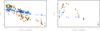 |
Fig. 1 Left panel: Ca i excitation rates (in s-1), log C, for electron impact (triangles) compared with the rates for H i collisions from quantum-mechanical calculations of MGB17 (filled circles) and B17u (rhombi) and compared with the scaled (SH = 0.1) Drawinian rates (open circles). Right panel: rates, log C, of the processes Ca i + e−→ Ca ii + 2e− and Ca i + H i → Ca ii + H− using similar symbols. The calculations were made with T = 5340 K, log Ne(cm-3) = 12.5, and log NH(cm-3) = 17. |
This study applies the NLTE method developed by Mashonkina et al. (2007, hereafter, Paper I) with the modifications concerning collisional rate computations. We briefly describe the atomic data we used. The model atom includes 63 levels of Ca i, 37 levels of Ca ii, and the ground state of Ca iii. For radiative transitions, we used accurate data on photoionisation cross-sections and transition probabilities from the Opacity Project (OP; see Seaton et al. 1994, for a general review), which are accessible in the TOPBASE3 database. In the SE calculations, inelastic collisions with electrons and hydrogen atoms leading to both excitation and ionisation are taken into account. For electron impact excitation, detailed results from the R-matrix calculations are available for ten transitions from the ground state in Ca i (Samson & Berrington 2001) and all the transitions between levels of the n ≤ 8 configurations of Ca ii (Meléndez et al. 2007). For the remaining bound-bound transitions, approximate formulae were used, namely, the impact parameter method (IPM, Seaton 1962a) for the allowed transitions and a collision strength of 1.0 and 2.0 for the optically forbidden transitions of Ca i and Ca ii, respectively. Electron impact ionisation cross-sections were calculated by applying the formula of Seaton (1962b) with threshold photoionisation cross-sections from the OP data.
A novelty of this research is that we account for the ion-pair production from the ground and excited states of Ca i and mutual neutralisation (charge-exchange reactions),
Ca i(nl) + H i ↔ Ca ii( ) + H− and H i impact excitation and de-excitation processes in Ca i, with the rate coefficients from quantum-mechanical calculations. The required data were taken from two different studies. Barklem (2016) developed a theoretical method for estimating cross-sections and rates for excitation and charge-transfer processes in low-energy hydrogen-atom collisions with neutral atoms, based on an asymptotic two-electron linear combination of atomic orbitals (LCAO) model of ionic-covalent interactions in the neutral atom-hydrogen-atom system and the multichannel Landau-Zener model. The rate coefficients used in our study are updated data, including a corrected H− wavefunction. Hereafter, we refer to these data as B17u. The rate coefficients of Mitrushchenkov et al. (2017) come from the accurate highly correlated ab initio electronic structure calculations followed by both the multichannel Landau-Zener model and the probability current method for nuclear dynamical calculations.
Figure 1 displays the excitation rates depending on the transition energy, Elu, and the ion-pair production rates depending on the level ionisation energy, χl, computed with the rate coefficients from two sources, MGB17 and B17u. Here, the data correspond to a kinetic temperature of T = 5340 K and an H i number density of log NH(cm-3) = 17 that are characteristic of the line-formation layers (log τ5000 = −0.52) in the model atmosphere with Teff/log g/[Fe/H] = 5780 K/3.70/−2.46. It is evident that for any common transition, both sources provide very similar collisional rates. Collisions with H i are more efficient compared with electron impacts in exciting the Elu ≾ 1.2 eV transitions, and the ion-pair production rates are substantially higher than the electron-impact ionisation rates for atomic levels with χl< 3.3 eV. In the next subsection, we inspect the influence of employing both MGB17 and B17u rate coefficients on the SE calculations and the calcium abundance determinations. The NLTE results in Sects. 4–6 are based on using the MGB17 data.
Collisions of Ca ii with H i were treated using the Drawinian rates that are scaled by a factor of SH = 0.1, as recommended in Paper I. We neglected collisions with H i for the Ca i transitions for which Barklem (2016) and Mitrushchenkov et al. (2017) did not provide rate coefficients, and also for the forbidden transitions in Ca ii.
2.2. Influence of inelastic collisions with H I on the statistical equilibrium of Ca I and calcium abundance determinations
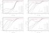 |
Fig. 2 Departure coefficients, b, for selected levels of Ca i from calculations using different treatment of H i collisions: a) – no H i collisions, that is, pure electronic collisions; b) – MGB17; c) – B17u; d) – Drawinian rates scaled by SH = 0.1. For the ground state of Ca ii, b = 1 (red continuous line) throughout the atmosphere. In each panel, the tick mark indicates the location of line centre optical depth unity for Ca i 6162 Å. Here, all the calculations were performed with a common model atmosphere: 5780/3.70/−2.46 and [Ca/Fe] = 0.4. |
We chose the VMP model atmosphere, namely, 5780/3.70/ −2.46, to investigate the influence of inelastic collisions with H i and their different treatment on the NLTE results for Ca i. The calculations were performed for five different line-formation scenarios based on pure electronic collisions (a), including H i collisions with the rate coefficients from MGB17 (b) and B17u (c), removing all the b–b transitions (e) in the MGB17 recipe, and for comparison, using the Drawinian rates scaled by SH = 0.1 (d). Figure 2 displays the departure coefficients, b = nNLTE/nLTE, for selected levels of Ca i in the scenarios (a)–(d). Here, nNLTE and nLTE are the statistical equilibrium and thermal (Saha-Boltzmann) number densities, respectively. It is worth noting that each of the triplet terms,  and
and  , is displayed as single level because the fine-splitting levels, which are treated explicitly in the model atom, reveal very similar departure coefficients. Since Ca ii is the majority species, variations in the treatment of Ca i + H i collisions nearly do not affect populations of the Ca ii levels. Therefore, only the ground state of Ca ii is plotted in Fig. 2.
As shown in the earlier NLTE studies (see Mashonkina et al. 2007, and references therein), the main NLTE mechanism for Ca i in the stellar parameter range, with which we are concerned here, is the ultra-violet (UV) over-ionisation caused by superthermal radiation of a non-local origin below the thresholds of the low excitation levels. We obtain that all levels of Ca i are underpopulated above log τ5000 = 0 in the 5780/3.70/−2.46 model atmosphere, independent of the treatment of collisional rates. As expected, the departures from LTE are smaller when collisions with H i are included. For example, in the atmospheric layers, where the line core of Ca i 6162 Å forms, at log τ5000 = −0.7, the departure coefficients of its lower ( ) and upper (
 ) levels amount to bl = 0.62 and bu = 0.62 in case of pure electronic collisions, while they are closer to unity in the MGB17 and B17u scenarios: bl = 0.875, bu = 0.954 and bl = 0.859, bu = 0.948, respectively. We find that the charge-exchange reactions influence the SE of Ca i to a greater extent than the H i-impact excitation. When we removed all the bound-bound (b–b) transitions in the MGB17 scenario, the departure coefficients changed only slightly. For example, we obtain b(
 ) = 0.862 and b() = 0.942 at log τ5000 = −0.7.
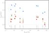 |
Fig. 3 NLTE abundance corrections for the lines of Ca i in the 5780/3.70/−2.46 and [Ca/Fe] = 0.4 model from calculations using pure electronic collisions (triangles) and including collisions with H i according to MGB17 (filled circles), B17u (filled rhombi), and MGB17 with no b–b transitions (open rhombi). For comparison, the NLTE corrections were computed with the scaled Drawinian rates (SH = 0.1, open circles). The vertical lines indicate positions of the following lines: 1 = 4425 Å, 2 = 5349 Å, 3 = 5588 Å, 4 = 5590 Å, 5 = 5857 Å, 6 = 6162 Å, 7 = 6169.5 Å, 8 = 6439 Å, 9 = 6493 Å, and 10 = 6499 Å. |
It is worth noting that although the Drawin (1968, 1969) formalism does not provide a realistic description of the physics involved, using the scaled Drawinian rates catches a main part of the effect of collisions with H i on the SE of Ca i. The bl = 0.845 and bu = 0.900 obtained for this option at log τ5000 = −0.7 are indeed closer to the MGB17 and B17u scenarios than to the case of pure electronic collisions.
Using various collisional recipes, we calculated the NLTE abundance corrections, ΔNLTE = log εNLTE−log εLTE, for the selected lines of Ca i in the 5780/3.70/−2.46 model (Fig. 3). They are mostly positive and larger for pure electronic collisions than in any line-formation scenario that includes collisions with H i, by up to 0.2 dex. In case of MGB17 and B17u, ΔNLTE does not exceed 0.11 and 0.17 dex, respectively, and the difference in ΔNLTE between the two options does not exceed 0.06 dex.
We note the particular case of Ca i 6439 Å, for which ΔNLTE is close to zero in case of MGB17, B17u, and MGB17 (no b–b) and even slightly negative in case of scaled Drawinian rates. Here, the same mechanisms are at work as first discussed by Drake (1991) for the [Fe/H] ≥−1 model atmospheres. The line wings are formed in deep layers where over-ionisation depopulates all Ca i levels, but the core of Ca i 6439 Å in the 5780/3.70/−2.46 model is formed at the depths, log τ5000 ≃ −0.7, where the upper level,  , of the transition is underpopulated to a greater extent than is the lower level,
  , because of photon losses in the line wings. The line source function drops below the Planck function at these depths, resulting in an enhanced absorption in the line core. The combined effect on the line strength is that the NLTE abundance correction is small. Sections 4 and 5 deal with similar phenomena in the formation of stellar Ca i lines, in particular, the resonance line.
Atmospheric parameters and obtained calcium NLTE and LTE abundances of the sample stars.
3. Stellar sample, observations, and atmospheric parameters
From the sample studied in Paper I, we selected HD 61421 (Procyon) and three metal-poor stars, HD 84937, HD 103095, and HD 140283, for which high-resolution observed spectra are available not only in the visible, but also in the IR regions. For these stars, we used the same observational material that was taken from Korn et al. (2003) and obtained with the fibre-fed échelle spectrograph FOCES (Pfeiffer et al. 1998) at the 2.2 m telescope of the Calar Alto observatory, with a spectral resolution of R = 65 000 (HD 140283 was observed at R = 40 000). For these data, the wavelength coverage is 4200–9000 Å. High-quality observations for Ca ii 8498 Å in HD 140283 were taken from the ESO UVESPOP survey (Bagnulo et al. 2003).
To this sample we added BD + 09°0352 and BD −13°3442. Their spectra are taken from the CFHT/ESPaDOnS archive4 (IDs 1424029 and 1515097-98, respectively). For these data, R = 68 000 and the wavelength coverage is 3715–9300 Å.
For the five MP stars, we used atmospheric parameters determined in our earlier study (Sitnova et al. 2015). In short, a combination of the photometric and spectroscopic methods was applied to derive effective temperatures and surface gravities. The spectroscopic analyses took advantage of the NLTE line-formation modelling for Fe i–ii, using the method described by Mashonkina et al. (2011). The iron abundance and microturbulence velocity, ξt, were determined simultaneously with log g.
Atmospheric parameters of Procyon are revised compared with those in Paper I. We adopted Teff = 6600 K from Boyajian et al. (2013), which is based on the bolometric flux measurements and the interferometric angular diameter improved by Chiavassa et al. (2012). To compute log g, we used the dynamical mass of 1.478 ± 0.012 solar mass as derived by Bond et al. (2015) and the linear radius of 2.0362 ± 0.0145 solar radius from Chiavassa et al. (2012). The iron abundance and microturbulence velocity were determined from the NLTE analysis of Fe i and Fe ii lines. The line list together with accurate line atomic data were compiled by Sitnova et al. (2015). Excluding the strong lines with an observed equivalent width of Wobs > 120 mÅ, we have 31 lines of Fe i and 15 lines lines of Fe ii. In a line-by-line differential analysis relative to the Sun, ξt = 1.8 km s-1 appears to provide the faintest slope of the Fe i-based abundance versus line strength trend. This value coincides with the earlier determination of Korn et al. (2003), which was also used in Paper I. The iron differential abundances based on lines of Fe i and Fe ii, [Fe/H]I = −0.01 ± 0.10 and [Fe/H]II = 0.05 ± 0.04, agree within 0.06 dex. Their mean is adopted as a final iron abundance.
Four of our sample stars were used by Heiter et al. (2015) as benchmark stars. For two of them, HD 84937 and Procyon, the adopted atmospheric parameters agree well in the two studies. For the other two stars, HD 103095 and HD 140283, their interferometric effective temperatures are not recommended by Heiter et al. (2015) to “be used as a reference for calibration or validation purposes”.
Stellar atmosphere parameters are given in Table 1.
4. Ca i versus Ca ii in the sample stars
Atomic data for the selected Ca i and Ca ii lines and the NLTE and LTE abundances, log ε⊙, determined from the line profiles in the Kitt Peak Solar Atlas (Kurucz et al. 1984).
In this section, we derive abundances from lines of Ca i and Ca ii in the Sun and selected stars and inspect the abundance differences between the two ionisation stages. For the stars, we applied a line-by-line differential NLTE and LTE approach, in the sense that stellar line abundances were compared with individual abundances of their solar counterparts. The NLTE abundances were calculated using rate coefficients for Ca i + H i collisions from Mitrushchenkov et al. (2017).
4.1. Line list, line atomic data, and the codes
We employed the line list and the line atomic data that were comprehensively tested in Paper I. In addition, Table 2 includes lines of Ca ii, which are used in Sect. 5 to derive Ca abundances of the UMP stars. Accurate laboratory gf-values are available for all investigated lines of Ca i and the low-excitation lines of Ca ii, with Eexc≤ 3.12 eV; the sources of data are indicated in Table 2. For high-excitation lines of Ca ii, with Eexc ≥ 7.05 eV, gf-values based on OP calculations were adopted. For the Ca ii IR triplet lines we account for the isotope structure with the isotope shifts measured by Nörtershäuser et al. (1998). For the Ca isotope abundance ratios the solar system values from Lodders et al. (2009) were adopted. Isotope shifts are much smaller (<10 mÅ) for the resonance lines in Ca i and Ca ii (Lucas et al. 2004) and we treat them as single lines. No data are available for the remaining Ca lines. We neglected the hyperfine structure of Ca lines because the fractional abundance of the only odd isotope 43Ca is very low (0.135%). For 17 Ca i lines, the van der Waals C6 values were computed from damping parameters given by Smith (1981) and based on the measured parameters for broadening by helium. For the remaining lines, we adopted C6 values based on the theory of collisional broadening by atomic hydrogen treated by Anstee & O’Mara (1995), Barklem & O’Mara (1997, 1998), and Barklem et al. (1998). Hereafter, these four important papers are referred to collectively as ABO. When the line is not available in any cited source, we rely on Kurucz’s5C6 values, which are accessible in the VALD database (Ryabchikova et al. 2015).
All our results are based on line-profile analysis. The theoretical spectra were computed with the code synthV-NLTE (Ryabchikova et al. 2016), which uses the departure coefficients from the DETAIL program (Butler & Giddings 1985). In turn, synthV-NLTE was integrated within the idl binmag3 code6 written by O. Kochukhov, finally allowing us to determine the best fit to the observed line profiles.
4.2. Analysis of solar Ca I and Ca II lines
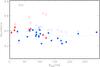 |
Fig. 4 Solar NLTE (filled symbols) and LTE (open symbols) calcium abundances, |

We used solar flux observations taken from the Kitt Peak Solar Atlas (Kurucz et al. 1984). The calculations were performed with the MARCS solar model atmosphere (Teff = 5777 K, log g = 4.44, [Fe/H] = 0) and a depth-independent microturbulence of 0.9 km s-1. When applying synthV-NLTE+binmag3, we fixed a spectral resolution at R = 500 000 and a rotation velocity at Vsini = 1.8 km s-1. Free parameters in line-profile fitting are the Ca abundance and the radial-tangential macroturbulence.
The LTE and NLTE abundances determined from 22 subordinate lines of Ca i and seven high-excitation lines of Ca ii are presented in Table 2 and Fig. 4. As discussed in Paper I, NLTE leads to strengthening most of Ca i lines in the solar atmosphere. The mechanisms are similar to those for Ca i 6439 Å in the 5780/3.70/−2.46 model (Sect. 2.2), that is, dropping the line source function below the Planck function at the line core formation depths results in the enhanced absorption in the line core, and this prevails over weakening the line wings formed in deep layers where over-ionisation depopulates all Ca i levels. The NLTE effects appear to be stronger when quantum-mechanical rate coefficients are applied for Ca i + H i collisions compared with the effect for the scaled (SH = 0.1) Drawinian rates. For example, the corresponding NLTE corrections amount to ΔNLTE = −0.07 and −0.03 dex for a moderate-strength line Ca i 6455 Å (Wobs = 59 mÅ).
The Ca i-based NLTE abundance obtained in this study, log εCaI = 6.33, is lower than the values calculated in Paper I with SH = 0 (no Ca i + H i collisions) and SH = 0.1, by 0.04 dex and 0.03 dex, respectively. This is mostly due to the different treatment of Ca i + H i collisions, but not using different solar model atmospheres, that is, to the MARCS model in this study and the MAFAGS (Fuhrmann et al. 1997) model in Paper I and to not neglecting Ca i 7326 Å in this study. Hereafter, the abundances are placed on a classical scale with log εH = 12.
For Ca ii, NLTE leads to fairly consistent abundances from seven high-excitation lines (Fig. 4), in contrast to LTE, where σ = 0.10 dex is twice larger. Hereafter, the sample standard deviation,  , determines the dispersion in the single line measurements around the mean, where N is the number of measured lines. We recall that Ca ii + H i collisions are treated in this study using the scaled (SH = 0.1) Drawinian rates. Therefore, the obtained mean abundance, log εCaII = 6.40, coincides with the corresponding value in Paper I. It is worth noting that a lower abundance, by 0.13 dex, is determined from the Ca ii 8498 Å line wings that are free of the NLTE effects. An abundance discrepancy between the Ca ii high-excitation lines and Ca ii 8498 Å can be caused by the uncertainty in predicted gf-values for the first group of lines or/and the uncertainty in predicted van der Waals damping constant for Ca ii 8498 Å.
The obtained Ca i-based NLTE abundance, log εCaI = 6.33, agrees well with the meteoritic value, log εmet = 6.31 ± 0.02 (Lodders et al. 2009). Our solar results can also be compared with calculations of Scott et al. (2015). Using different line lists (11 lines of Ca i and 5 lines of Ca ii) compared with ours and the same solar MARCS model, they obtained the NLTE abundances log εCaI = 6.26 and log εCaII = 6.28. Their recommended solar Ca abundance, log εCa = 6.32 ± 0.03, is based on the LTE abundances calculated with the 3D hydrodynamic model of the solar photosphere, to which the NLTE corrections from the 1D model were applied.
4.3. Stellar abundances from lines of Ca I and Ca II
When we applied synthV-NLTE+binmag3, we fixed a spectral resolution for a given star at the value indicated in Sect. 3. Only for Procyon, rotational broadening, with Vsini = 2.6 km s-1 from Fuhrmann (1998), and broadening by macroturbulence were treated separately. The remaining stars are slow rotators, Vsini ≾ 1.5 km s-1, and therefore the rotational velocity and macroturbulence value cannot be separated at the spectral resolving power of our spectra. We therefore consider their overall effect as radial-tangential macroturbulence, and together with the Ca abundance, they are free parameters in line-profile fitting.
For each star, we determined abundances from the subordinate lines of Ca i, the high-excitation lines of Ca ii, where available, and for the MP stars, from Ca ii 8498 Å. Table 1 presents the mean NLTE and LTE abundances. For Ca i, the difference in the mean abundance between the two NLTE scenarios exceeds 0.02 dex at no point. The NLTE data in Table 1 correspond to the MGB17 scenario.
We first focus on Procyon, for which our earlier study (Mashonkina et al. 2007) obtained an abundance difference of more than 0.2 dex between the two ionisation stages, Ca i and Ca ii, independently of the line-formation scenario, and the determined Ca i-based abundance was clearly subsolar, although a success was achieved in removing a steep trend with line strength among strong Ca i lines seen in LTE. In this study, we applied a 90 K higher effective temperature, and this appears the key to the solution of the abundance problems. The NLTE abundances from Ca i and Ca ii agree within 0.06 dex (Table 1), and [Ca/H]I = −0.07 (σ = 0.05) is close to the solar value. As in Paper I, we obtained consistent NLTE abundances from Ca i lines of different strength, in contrast to the LTE abundances, which reveal a steep increasing trend at Wobs> 110 mÅ (Fig. 5).
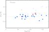 |
Fig. 5 NLTE (filled symbols) and LTE (open symbols) [Ca/H] abundances determined from the Ca i (circles) and Ca ii (triangles) lines in Procyon. Note the steep trend of the Ca i-based LTE values with line strength above Wobs = 100 mÅ. The dotted line indicates the mean [Ca/Fe]I NLTE value. |
NLTE largely removes the line-to-line scatter for Ca ii.
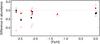 |
Fig. 6 NLTE (filled symbols) and LTE (open symbols) differences between [Ca/H]I and [Ca/H]II for the sample stars. The squares and triangles correspond to the high-excitation lines of Ca ii and Ca ii 8498 Å, respectively. |
NLTE also works well for our MP stars. For every star, it reduces the line-to-line scatter for both Ca i and Ca ii compared with LTE. NLTE leads to higher abundances from lines of Ca i and lower abundance from Ca ii 8498 Å, such that these two abundance indicators provide consistent results, in contrast to LTE, where the abundance difference (Ca i−Ca ii 8498 Å) grows towards lower metallicity and reaches −0.46 dex in BD −13°3442 ([Fe/H] = −2.62, Fig. 6).
For Ca ii 8912, 8927 Å in the VMP stars, NLTE leads to strengthened lines and negative NLTE abundance corrections, which are smaller in absolute value than those for the solar lines, resulting in positive abundance differences, [Ca/H]NLTE – [Ca/H]LTE. Their magnitudes are as large as the magnitude for the Ca i lines. Therefore, the NLTE and LTE abundance differences [Ca/H]I – [Ca/H]II are close together for each star (Fig. 6). They are within 1σ for BD + 09°0352 and BD −13°3442, but amount to −0.17 and −0.22 dex for HD 84937 and HD 140283, respectively.
To determine whether the discrepancy in abundance between different lines of Ca ii might be caused by an uncertainty in log g, we calculated NLTE abundances of HD 84937 using an 0.1 dex lower surface gravity. A decrease of log g leads to stronger Ca ii lines and lower derived abundances. For Ca ii 8912, 8927 Å, the abundance shifts amount to −0.04 dex and −0.03 dex, respectively. The NLTE abundance from Ca ii 8498 Å is the same regardless of whether we use log g = 4.09 or 3.99. A change of 0.1 dex in log g for HD 84937 leads to a minor change of 0.04 dex in the NLTE abundance difference between Ca ii lines and does not help to achieve consistent abundances from different lines of Ca ii.
5. Ca i versus Ca ii in the UMP stars
Atmospheric parameters and obtained calcium NLTE and LTE abundances of the UMP stars.
In this section, we determine Ca absolute abundances of the three UMP stars listed in Table 3. Five lines of Ca ii, that is, the resonance line at 3933 Å, the IR triplet lines, and the low-excitation line at 3706 Å, were observed in HE 0557-4840 and two lines, Ca ii 3933 and 8498 Å, in HE 1327-2326. We inspected whether different lines of Ca ii in a given star yield consistent abundances. In all three stars, neutral calcium is represented only by the Ca i 4226 Å resonance. For each star, we checked the Ca i/Ca ii ionisation equilibrium with given atmospheric parameters.
For HE 0557-4840, HE 0107-5240, and HE 1327-2326, we use reduced spectra from the VLT/UVES7 archive (IDs 380.D-0040(A); 0.D-0009(A), 076.D-0165(A); and 075.D-0048(A), 077.D-0035(A), respectively) and the earlier study of Korn et al. (2009), in which one of us (L.M.) took part. Atmospheric parameters were taken from the literature, as indicated in Table 3.
Pronounced departures from LTE are found for the Ca ii IR triplet lines in HE 0557-4840 (Fig. 7), such that the observed profile cannot be reproduced in LTE for any of the lines. First, we note the shift in wavelength between the NLTE and LTE profile that is due to different NLTE affecting the different isotopic components of the line. Second, the LTE profile is much shallower than the observed profile, even when no external broadening by macro-turbulence and instrumental broadening is applied, as shown for Ca ii 8542 and 8662 Å. When using the observed equivalent widths, we obtain an LTE abundance that is substantially higher than the NLTE abundance, for example, by 0.67 dex for Ca ii 8498 Å. In contrast, NLTE leads to weakening Ca ii 3706 Å and positive abundance correction of ΔNLTE = 0.18 dex. For Ca ii 3933 Å, the NLTE effects are minor, with ΔNLTE< 0.01 dex. We find fairly consistent NLTE abundances from different lines of Ca ii in HE 0557-4840, with σ = 0.05 dex (Table 3). The Ca i resonance line gives a lower NLTE abundance than that deduced from Ca ii lines, by 0.26 dex. These results differ from those of Norris et al. (2007) because (i) using accurate quantum-mechanical data on Ca i + H i collisions leads to smaller positive NLTE correction for Ca i 4226 Å compared with that for the scaled Drawinian rates, by 0.10 dex in the MGB17 scenario; (ii) we used absolute, but not differential abundances; (iii) in addition to Ca ii 3933 and 3706 Å, we used the Ca ii IR triplet lines.
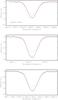 |
Fig. 7 Best NLTE (continuous curve) fits of the Ca ii IR triplet lines in HE 0557-4840 (open circles). The obtained NLTE abundances are log εCa = 2.21, 2.13, and 2.15 for Ca ii 8498, 8542, and 8662 Å, respectively. The LTE profiles (dashed curve) were computed with 0.57 dex higher Ca abundance compared with the corresponding NLTE one. See text for more details. |
Both lines of Ca ii and the Ca i resonance line in HE 1327-2326 give NLTE abundances that are consistent within 0.02 dex, in contrast to LTE, where the abundance difference between Ca ii and Ca i amounts to 0.42 dex.
For HE 0107-5240, NLTE largely removes an abundance discrepancy of 0.47 dex between Ca ii 3933 Å and Ca i 4226 Å, which was obtained at the LTE assumption.
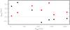 |
Fig. 8 NLTE abundance corrections for Ca i 4226 Å (squares) in most of the investigated MP stars as a function of line strength and the corresponding absolute abundance differences between Ca ii and Ca i 4226 Å (circles) and between the Ca i subordinate and resonance lines (triangles). |
In Fig. 8 we display an abundance difference between Ca i 4226 Å and Ca ii lines not only for the UMP stars, but also for our four VMP stars. For the latter group, we used the abundances from Ca ii 8498 Å, which agree well with the values deduced from the Ca i subordinate lines (Sect. 4.3) and thus are reliable. The Ca i resonance line yields a slightly lower abundance than the Ca ii-based one, by up to 0.1 dex, when it is either weak (Wobs = 2.7 and 25 mÅ in HE 1327-2326 and HE 0107-5240, respectively) or strong enough (Wobs> 150 mÅ in HD 84937 and BD + 09°0352). In the other three stars, HD 140283, BD −13°3442, and HE 0557-4840, Ca i 4226 Å is of moderate strength and gives substantially lower abundance than that from Ca ii lines and also from subordinate lines of Ca i, where available. For example, in HD 140283, the abundance difference between Ca i resonance and subordinate lines amounts to −0.32 dex and −0.33 dex between Ca i 4226 Å and Ca ii 8498 Å. The problem of the underestimated abundance from Ca i 4226 Å was noted in our Paper I for the [Fe/H] ≃ −2 dwarf stars and highlighted by Spite et al. (2012) for their sample of VMP turnoff stars and giants.
To clarify the situation with Ca i 4226 Å, we plot in Fig. 9 the departure coefficients of the lower ( ) and upper (
 ) levels of the corresponding transition in three model atmospheres of different metallicity. We chose BD+ 09°0352 ([Fe/H] = −2.09), BD−13°3442 ([Fe/H] = −2.62), and HE 0107-5240 ([Fe/H] = −5.3). For comparison, departure coefficients of the lower and upper levels of Ca i 6162 Å (–
 ) are also shown. In the [Fe/H] = −5.3 model, Ca i 4226 Å forms in deep atmospheric layers where the overall over-ionisation of Ca i leads to a weakened line (bottom row of Fig. 9) and positive NLTE abundance correction (Fig. 8). In contrast, in the [Fe/H] = −2.09 model, the core of the resonance line forms in the uppermost atmospheric layers, where b() <b() due to photon loss in the line itself and the line source function is smaller than the Planck function, resulting in enhanced absorption in the line core. However, at this metallicity, the line has broad wings that form in deep atmospheric layers and are weakened by over-ionisation of Ca i. This compensates, in part, for the NLTE effects in the line core and results in an only slightly negative NLTE abundance correction of ΔNLTE = −0.04 dex. In the [Fe/H] = −2.62 model, Ca i 4226 Å nearly looses its line wings, and enhanced absorption in the line core determines the NLTE effects on the total strength of the line.
 |
Fig. 9 Top row: departure coefficients for selected levels of Ca i and Ca ii as a function of log τ5000 in the models representing atmospheres of BD + 09°0352, BD −13°3442, and HE 0107-5240. Tick marks indicate the locations of line centre optical depth unity for Ca i 4226 Å (1) and Ca i 6162 Å (2). Bottom row: NLTE (continuous curve) and LTE (dashed curve) theoretical profiles of Ca i 4226 Å in the corresponding models. |
We thus understand why in a certain range of the Ca abundance, NLTE modelling leads to a too strong Ca i 4226 Å line and to a too low abundance derived from this line, but we have no tool to influence the SE of Ca i in the uppermost atmospheric layers where the UV over-ionisation and photon escapes in the resonance line decide the situation.
Based on this analysis, we suggest that NLTE modelling provides reliable results for Ca i 4226 Å when the calcium abundance is low, [Ca/H] ≾ −5, and the Ca i/Ca ii ionisation equilibrium method can successfully be applied to determine surface gravities of the hyper metal-poor stars. For example, if the abundance difference Ca i – Ca ii is accurate within 0.1 dex, the uncertainty in log g of HMP turn-off star does not exceed 0.2 dex.
6. NLTE abundance corrections for lines of Ca i depending on stellar parameters
With the MGB17 collisional data, we computed the NLTE abundance corrections for 28 lines of Ca i in the grid of MARCS model atmospheres, where an effective temperature varies between 5000 K and 6500 K, with a 250 K step, and surface gravity between log g = 2.5 and 4.5, with a 0.5 step. The metallicity ranges between [Fe/H] = 0 and −4. In part, the obtained results are displayed in Fig. 10. The entire data set is available in machine-readable form8.
Comments on Fig. 10.
-
The NLTE corrections are not provided for model atmosphereswhere a given line is weak, with an equivalent width smaller than3 mÅ. Even the strongest subor-dinate lines of Ca i are weak in the[Fe/H] = −4 models.
-
A common feature of most Ca i lines is the change in sign of the NLTE abundance correction when moving from the solar metallicity and mildly metal-poor model atmospheres, where ΔNLTE< 0, to the very metal-poor ones, where ΔNLTE> 0. When a line is strong, its wings are weakened, but the core is stronger than in the LTE case. The value and sign of ΔNLTE are defined by a relative contribution of the core and the wings to the overall line strength. When the line becomes weak as a result of the decreasing Ca abundance, NLTE leads to depleted total absorption in the line and to a positive abundance correction. The metallicity at which a change in sign occurs is different for different lines, and for a given line, it depends on atmospheric Teff and log g. In the Teff = 5750 K models, ΔNLTE is only positive throughout the investigated metallicity range for Ca i 6161 and 6169.0 Å.
-
In general, the NLTE effects grow towards lower surface gravity. For Ca i 6161 and 6169.0 Å, ΔNLTE grows towards lower metallicity in the entire metallicity range and, for the remaining lines, at [Fe/H] < −1.5.
It is worth noting that the NLTE abundance corrections for lines of Ca i in the cool giant model atmospheres (4000 K ≤ Teff ≤ 5000 K, 0.5 ≤ log g≤ 2.5, −4 ≤ [Fe/H] ≤ 0) were computed by Mashonkina et al. (2016) using rate coefficients for Ca i + H i collisions from quantum-mechanical calculations of Belyaev et al. (2016). The data are accessible online9, and can be downloaded in machine-readable form10. We have inspected differences in ΔNLTE between applying data of Belyaev et al. (2016) and data from Mitrushchenkov et al. (2017). They are minor in most cases. For example, in the 4500/1.5/−3 model, the NLTE abundance corrections based on the MGB17 data are smaller, by 0.02–0.03 dex, for the W ≾ 30 mÅ lines, but larger, by 0.02–0.03 dex, for the stronger lines compared with the corresponding values computed with the rate coefficients from Belyaev et al. (2016).
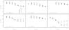 |
Fig. 10 NLTE (MGB17) abundance corrections for selected lines of Ca i depending on metallicity and surface gravity in the models with common Teff = 5750 K. Different symbols correspond to different surface gravities: log g = 2.5 (asterisks), 3.0 (circles), 3.5 (rhombi), 4.0 (squares), and 4.5 (triangles). |
7. Conclusions and recommendations
We performed the NLTE calculations for Ca i–ii with the updated model atom that includes inelastic Ca i+H i collisions using accurate rate coefficients from quantum-mechanical calculations of Mitrushchenkov et al. (2017). For Ca ii, we still applied the classical Drawinian rates scaled by SH = 0.1. For the model atmosphere representative of the VMP turnoff stars, 5780/3.7/−2.46, we showed that including H i collisions substantially reduces the over-ionisation of Ca i in the line formation layers compared with the case of pure electronic collisions, such that the NLTE abundance corrections become smaller, by 0.08 to 0.20 dex, for different Ca i lines. The calculations of Mitrushchenkov et al. (2017) and Barklem (2016, updated) provide very similar rate coefficients for Ca i+H i collisions.
The NLTE abundances based on the MGB17 collisional data were derived from the Ca i subordinate lines in the Sun, Procyon, and five MP stars in the −2.62 ≤ [Fe/H] ≤ −1.26 metallicity range. In order to inspect the Ca i/Ca ii ionisation equilibrium with given atmospheric parameters, we determined abundances from the high-excitation lines of Ca ii, and for the MP stars, also from Ca ii 8498 Å. The analysis of 22 solar Ca i lines with the MARCS solar model atmosphere yields the NLTE abundance log εCaI = 6.33 (σ = 0.06 dex), in line with the meteoritic value of Lodders et al. (2009) and the photospheric abundance based on the 3D+NLTE calculations of Scott et al. (2015). The NLTE abundance calculated from solar high-excitation lines of Ca ii, log εCaII = 6.40 (σ = 0.05 dex), is higher than that from the Ca ii 8498 Å line wing fit, by 0.13 dex. For the stars, we determined the differential NLTE and LTE abundances relative to the Sun. The obtained results can be summarised as follows.
-
For both Ca i andCa ii in every star including theSun, NLTE leads to smaller line-to-line scatter, such thatσ reduces compared with the LTE one, by up to a factor of 2.5.
-
For Procyon, NLTE removes a steep trend with line strength among strong Ca i lines seen in LTE.
-
For Procyon, we achieve NLTE abundances consistent within 0.06 dex from the two ionisation stages, Ca i and Ca ii.
-
In each of the five MP stars, Ca ii 8498 Å yields an NLTE abundance that agrees well with that from the Ca i subordinate lines. For comparison, the difference in LTE abundances grows towards lower metallicity and reaches 0.46 dex in BD −13°3442 ([Fe/] = −2.62).
-
For the four VMP stars, NLTE largely removes obvious abundance discrepancies between the high-excitation lines of Ca ii and Ca ii 8498 Å obtained under LTE assumption.
We thus strongly recommend to apply the NLTE approach to Ca abundance determinations. This is important for any individual star because the magnitude and sign of the NLTE abundance correction can be different for different lines of Ca i and Ca ii and for stellar samples covering wide metallicity ranges. The SE equilibrium calculations have to include inelastic Ca i + H i collisions.
With the updated model atom, we investigate the formation of the Ca i 4226 Å resonance line in the [Fe/H] < −2 stars, where it has a purely photospheric origin. In the four stars with −2.3 < [Ca/H] < −1.8 (−2.62 ≤ [Fe/H] ≤−2.09), Ca i 4226 Å is strong enough, with Wobs ≥ 113 mÅ, and NLTE predicts a weakening of the line wings and strengthening of the line core compared with the LTE case, resulting in negative NLTE abundance correction. A relative contribution of the core to the overall line strength grows with decreasing Ca abundance, and ΔNLTE increases in absolute value. In these stars, the Ca i resonance line yields a lower abundance than the abundance from the subordinate lines, by 0.08 to 0.32 dex. We can explain why the abundance derived from Ca i 4226 Å is underestimated, but cannot influence the photon loss in the Ca i resonance line in the uppermost atmospheric layers that is the driver of strengthening the line core, which results in a negative NLTE abundance correction.
When we decrease the Ca abundance to [Ca/H] ≃−4.4, like that of the UMP star HE 0557-4840, the line core formation depth shifts to deep atmospheric layers, where over-ionisation of Ca i determines the depleted total absorption in the line and a positive abundance correction. Nevertheless, the NLTE abundance obtained from Ca i 4226 Å in HE 0557-4840 is lower than that from five Ca ii lines, by 0.26 dex.
The NLTE effects for Ca i 4226 Å grow towards lower Ca abundance, and we computed large positive NLTE corrections of ΔNLTE = 0.34 and 0.25 dex for the two HMP stars HE 0107-5240 and HE 1327-2326, respectively. For each of them, the NLTE abundances from the Ca i resonance line and the Ca ii lines are found to be consistent. Thus, the Ca i/Ca ii ionisation equilibrium method can successfully be applied to determine surface gravities of hyper metal-poor stars.
Acknowledgments
This study is based on observations made with ESO Telescopes at the La Silla Paranal Observatory under programme IDs 075.D-0048(A), 077.D-0035(A), 0.D-0009(A), 076.D-0165(A), and 380.D-0040(A) and with the Canada-France-Hawaii Telescope under programme IDs 1424029 and 1515097-98. This research used the services of the ESO Science Archive Facility and the facilities of the Canadian Astronomy Data Centre operated by the National Research Council of Canada with the support of the Canadian Space Agency. The authors acknowledge financial support from the Russian Scientific Foundation (grant 17-13-01144). We made use the MARCS and VALD databases. We thank Oleg Kochukhov for providing the idl binmag3 code.
References
- Andretta, V., Busà, I., Gomez, M. T., & Terranegra, L. 2005, A&A, 430, 669 [NASA ADS] [CrossRef] [EDP Sciences] [Google Scholar]
- Anstee, S. D., & O’Mara, B. J. 1995, MNRAS, 276, 859 [NASA ADS] [CrossRef] [Google Scholar]
- Aoki, W., Frebel, A., Christlieb, N., et al. 2006, ApJ, 639, 897 [NASA ADS] [CrossRef] [Google Scholar]
- Bagnulo, S., Jehin, E., Ledoux, C., et al. 2003, The Messenger, 114, 10 [NASA ADS] [Google Scholar]
- Barklem, P. S. 2016, Phys. Rev. A, 93, 042705 [NASA ADS] [CrossRef] [Google Scholar]
- Barklem, P. S., & O’Mara, B. J. 1997, MNRAS, 290, 102 [Google Scholar]
- Barklem, P. S., & O’Mara, B. J. 1998, MNRAS, 300, 863 [NASA ADS] [CrossRef] [Google Scholar]
- Barklem, P. S., O’Mara, B. J., & Ross, J. E. 1998, MNRAS, 296, 1057 [Google Scholar]
- Battaglia, G., Helmi, A., Tolstoy, E., et al. 2008, ApJ, 681, L13 [NASA ADS] [CrossRef] [Google Scholar]
- Belyaev, A. K., Yakovleva, S. A., Guitou, M., et al. 2016, A&A, 587, A114 [NASA ADS] [CrossRef] [EDP Sciences] [Google Scholar]
- Bond, H. E., Gilliland, R. L., Schaefer, G. H., et al. 2015, ApJ, 813, 106 [NASA ADS] [CrossRef] [Google Scholar]
- Bonifacio, P., Caffau, E., Spite, M., et al. 2015, A&A, 579, A28 [NASA ADS] [CrossRef] [EDP Sciences] [Google Scholar]
- Boyajian, T. S., von Braun, K., van Belle, G., et al. 2013, ApJ, 771, 40 [NASA ADS] [CrossRef] [Google Scholar]
- Butler, K., & Giddings, J. 1985, Newsletter on the analysis of astronomical spectra, No. 9, University of London [Google Scholar]
- Caffau, E., Bonifacio, P., François, P., et al. 2011, Nature, 477, 67 [NASA ADS] [CrossRef] [PubMed] [Google Scholar]
- Caffau, E., Bonifacio, P., François, P., et al. 2012, A&A, 542, A51 [NASA ADS] [CrossRef] [EDP Sciences] [Google Scholar]
- Cayrel, R., Depagne, E., Spite, M., et al. 2004, A&A, 416, 1117 [NASA ADS] [CrossRef] [EDP Sciences] [Google Scholar]
- Chiavassa, A., Bigot, L., Kervella, P., et al. 2012, A&A, 540, A5 [NASA ADS] [CrossRef] [EDP Sciences] [Google Scholar]
- Christlieb, N., Bessell, M. S., Beers, T. C., et al. 2002, Nature, 419, 904 [NASA ADS] [CrossRef] [PubMed] [Google Scholar]
- Christlieb, N., Gustafsson, B., Korn, A., et al. 2004, ApJ, 603, 708 [NASA ADS] [CrossRef] [Google Scholar]
- Cohen, J. G., Christlieb, N., Thompson, I., et al. 2013, ApJ, 778, 56 [NASA ADS] [CrossRef] [Google Scholar]
- Drake, J. J. 1991, MNRAS, 251, 369 [NASA ADS] [CrossRef] [Google Scholar]
- Drawin, H.-W. 1968, Z. Phys., 211, 404 [NASA ADS] [CrossRef] [EDP Sciences] [Google Scholar]
- Drawin, H. W. 1969, Z. Phys., 225, 483 [NASA ADS] [CrossRef] [EDP Sciences] [Google Scholar]
- Drozdowski, R., Ignaciuk, M., Kwela, J., & Heldt, J. 1997, Z. Phys. D Atoms Molecules Clusters, 41, 125 [CrossRef] [Google Scholar]
- Frebel, A., Aoki, W., Christlieb, N., et al. 2005, Nature, 434, 871 [NASA ADS] [CrossRef] [PubMed] [Google Scholar]
- Frebel, A., Chiti, A., Ji, A. P., Jacobson, H. R., & Placco, V. M. 2015, ApJ, 810, L27 [NASA ADS] [CrossRef] [Google Scholar]
- Fuhrmann, K. 1998, A&A, 338, 161 [NASA ADS] [Google Scholar]
- Fuhrmann, K., Pfeiffer, M., Frank, C., Reetz, J., & Gehren, T. 1997, A&A, 323, 909 [NASA ADS] [Google Scholar]
- Gustafsson, B., Edvardsson, B., Eriksson, K., et al. 2008, A&A, 486, 951 [NASA ADS] [CrossRef] [EDP Sciences] [Google Scholar]
- Heiter, U., Jofré, P., Gustafsson, B., et al. 2015, A&A, 582, A49 [NASA ADS] [CrossRef] [EDP Sciences] [PubMed] [Google Scholar]
- Idiart, T., & Thévenin, F. 2000, ApJ, 541, 207 [NASA ADS] [CrossRef] [Google Scholar]
- Jorgensen, U. G., Carlsson, M., & Johnson, H. R. 1992, A&A, 254, 258 [NASA ADS] [Google Scholar]
- Keller, S. C., Bessell, M. S., Frebel, A., et al. 2014, Nature, 506, 463 [NASA ADS] [CrossRef] [PubMed] [Google Scholar]
- Korn, A. J., Shi, J., & Gehren, T. 2003, A&A, 407, 691 [NASA ADS] [CrossRef] [EDP Sciences] [Google Scholar]
- Korn, A. J., Richard, O., Mashonkina, L., et al. 2009, ApJ, 698, 410 [NASA ADS] [CrossRef] [Google Scholar]
- Kurucz, R. L., Furenlid, I., Brault, J., & Testerman, L. 1984, Solar flux atlas from 296 to 1300 nm (New Mexico: National Solar Observatory) [Google Scholar]
- Lodders, K., Plame, H., & Gail, H.-P. 2009, in Landolt-Börnstein – Group VI Astronomy and Astrophysics Numerical Data and Functional Relationships in Science and Technology, Volume 4B: Solar System, ed. J. E. Trümper, 44 [Google Scholar]
- Lucas, D. M., Ramos, A., Home, J. P., et al. 2004, Phys. Rev. A, 69, 012711 [NASA ADS] [CrossRef] [Google Scholar]
- Mashonkina, L., Korn, A. J., & Przybilla, N. 2007, A&A, 461, 261 (Paper I) [NASA ADS] [CrossRef] [EDP Sciences] [Google Scholar]
- Mashonkina, L., Gehren, T., Shi, J.-R., Korn, A. J., & Grupp, F. 2011, A&A, 528, A87 [NASA ADS] [CrossRef] [EDP Sciences] [Google Scholar]
- Mashonkina, L., Sitnova, T., & Pakhomov, Y. 2016, Astron. Lett., 42, 606 [NASA ADS] [CrossRef] [Google Scholar]
- Meléndez, M., Bautista, M. A., & Badnell, N. R. 2007, A&A, 469, 1203 [NASA ADS] [CrossRef] [EDP Sciences] [Google Scholar]
- Merle, T., Thévenin, F., Pichon, B., & Bigot, L. 2011, MNRAS, 418, 863 [NASA ADS] [CrossRef] [Google Scholar]
- Mitrushchenkov, A., Guitou, M., Belyaev, A. K., et al. 2017, J. Chem. Phys., 146, 014304 [NASA ADS] [CrossRef] [Google Scholar]
- Moore, C. E. 1972, A multiplet table of astrophysical interest – Pt.1: Table of multiplets – Pt.2: Finding list of all lines in the table of multiplets [Google Scholar]
- Norris, J., Christlieb, N., Korn, A., et al. 2007, ApJ, 670, 774 [NASA ADS] [CrossRef] [Google Scholar]
- Nörtershäuser, W., Blaum, K., Icker, K., et al. 1998, Eur. Phys. J. D, 2, 33 [NASA ADS] [CrossRef] [EDP Sciences] [Google Scholar]
- Perryman, M. A. C., de Boer, K. S., Gilmore, G., et al. 2001, A&A, 369, 339 [NASA ADS] [CrossRef] [EDP Sciences] [Google Scholar]
- Pfeiffer, M. J., Frank, C., Baumueller, D., Fuhrmann, K., & Gehren, T. 1998, A&AS, 130, 381 [NASA ADS] [CrossRef] [EDP Sciences] [Google Scholar]
- Ryabchikova, T., Piskunov, N., Kurucz, R. L., et al. 2015, Phys. Scr., 90, 054005 [NASA ADS] [CrossRef] [Google Scholar]
- Ryabchikova, T., Piskunov, N., Pakhomov, Y., et al. 2016, MNRAS, 456, 1221 [NASA ADS] [CrossRef] [Google Scholar]
- Rybicki, G. B., & Hummer, D. G. 1991, A&A, 245, 171 [NASA ADS] [Google Scholar]
- Rybicki, G. B., & Hummer, D. G. 1992, A&A, 262, 209 [NASA ADS] [Google Scholar]
- Samson, A. M., & Berrington, K. A. 2001, Atomic Data and Nuclear Data Tables, 77, 87 [Google Scholar]
- Scott, P., Grevesse, N., Asplund, M., et al. 2015, A&A, 573, A25 [NASA ADS] [CrossRef] [EDP Sciences] [Google Scholar]
- Seaton, M. J. 1962a, Proc. Phys. Soc., 79, 1105 [NASA ADS] [CrossRef] [Google Scholar]
- Seaton, M. J. 1962b, in Atomic and Molecular Processes, ed. D. R. Bates, 375 [Google Scholar]
- Seaton, M. J., Yan, Y., Mihalas, D., & Pradhan, A. K. 1994, MNRAS, 266, 805 [NASA ADS] [CrossRef] [Google Scholar]
- Sitnova, T., Zhao, G., Mashonkina, L., et al. 2015, ApJ, 808, 148 [Google Scholar]
- Smith, G. 1981, A&A, 103, 351 [NASA ADS] [Google Scholar]
- Smith, G. 1988, J. Phys. B At. Mol. Phys., 21, 2827 [NASA ADS] [CrossRef] [Google Scholar]
- Smith, W. W., & Gallagher, A. 1966, Phys. Rev., 145, 26 [NASA ADS] [CrossRef] [Google Scholar]
- Smith, G., & O’Neill, J. A. 1975, A&A, 38, 1 [NASA ADS] [Google Scholar]
- Smith, G., & Raggett, D. S. J. 1981, J. Phys. B At. Mol. Phys., 14, 4015 [NASA ADS] [CrossRef] [Google Scholar]
- Spite, M., Andrievsky, S. M., Spite, F., et al. 2012, A&A, 541, A143 [NASA ADS] [CrossRef] [EDP Sciences] [Google Scholar]
- Starkenburg, E., Hill, V., Tolstoy, E., et al. 2010, A&A, 513, A34 [NASA ADS] [CrossRef] [EDP Sciences] [Google Scholar]
- Steenbock, W., & Holweger, H. 1984, A&A, 130, 319 [NASA ADS] [Google Scholar]
- Steinmetz, M., Zwitter, T., Siebert, A., et al. 2006, AJ, 132, 1645 [NASA ADS] [CrossRef] [Google Scholar]
- Theodosiou, C. E. 1989, Phys. Rev. A, 39, 4880 [NASA ADS] [CrossRef] [Google Scholar]
- Watanabe, T., & Steenbock, W. 1985, A&A, 149, 21 [NASA ADS] [Google Scholar]
- Zhao, G., Mashonkina, L., Yan, H. L., et al. 2016, ApJ, 833, 225 [NASA ADS] [CrossRef] [Google Scholar]
All Tables
Atmospheric parameters and obtained calcium NLTE and LTE abundances of the sample stars.
Atomic data for the selected Ca i and Ca ii lines and the NLTE and LTE abundances, log ε⊙, determined from the line profiles in the Kitt Peak Solar Atlas (Kurucz et al. 1984).
Atmospheric parameters and obtained calcium NLTE and LTE abundances of the UMP stars.
All Figures
|
Fig. 1 Left panel: Ca i excitation rates (in s-1), log C, for electron impact (triangles) compared with the rates for H i collisions from quantum-mechanical calculations of MGB17 (filled circles) and B17u (rhombi) and compared with the scaled (SH = 0.1) Drawinian rates (open circles). Right panel: rates, log C, of the processes Ca i + e−→ Ca ii + 2e− and Ca i + H i → Ca ii + H− using similar symbols. The calculations were made with T = 5340 K, log Ne(cm-3) = 12.5, and log NH(cm-3) = 17. |
| In the text | |
|
Fig. 2 Departure coefficients, b, for selected levels of Ca i from calculations using different treatment of H i collisions: a) – no H i collisions, that is, pure electronic collisions; b) – MGB17; c) – B17u; d) – Drawinian rates scaled by SH = 0.1. For the ground state of Ca ii, b = 1 (red continuous line) throughout the atmosphere. In each panel, the tick mark indicates the location of line centre optical depth unity for Ca i 6162 Å. Here, all the calculations were performed with a common model atmosphere: 5780/3.70/−2.46 and [Ca/Fe] = 0.4. |
| In the text | |
|
Fig. 3 NLTE abundance corrections for the lines of Ca i in the 5780/3.70/−2.46 and [Ca/Fe] = 0.4 model from calculations using pure electronic collisions (triangles) and including collisions with H i according to MGB17 (filled circles), B17u (filled rhombi), and MGB17 with no b–b transitions (open rhombi). For comparison, the NLTE corrections were computed with the scaled Drawinian rates (SH = 0.1, open circles). The vertical lines indicate positions of the following lines: 1 = 4425 Å, 2 = 5349 Å, 3 = 5588 Å, 4 = 5590 Å, 5 = 5857 Å, 6 = 6162 Å, 7 = 6169.5 Å, 8 = 6439 Å, 9 = 6493 Å, and 10 = 6499 Å. |
| In the text | |
|
Fig. 4 Solar NLTE (filled symbols) and LTE (open symbols) calcium abundances, |
| In the text | |
|
Fig. 5 NLTE (filled symbols) and LTE (open symbols) [Ca/H] abundances determined from the Ca i (circles) and Ca ii (triangles) lines in Procyon. Note the steep trend of the Ca i-based LTE values with line strength above Wobs = 100 mÅ. The dotted line indicates the mean [Ca/Fe]I NLTE value. |
| In the text | |
|
Fig. 6 NLTE (filled symbols) and LTE (open symbols) differences between [Ca/H]I and [Ca/H]II for the sample stars. The squares and triangles correspond to the high-excitation lines of Ca ii and Ca ii 8498 Å, respectively. |
| In the text | |
|
Fig. 7 Best NLTE (continuous curve) fits of the Ca ii IR triplet lines in HE 0557-4840 (open circles). The obtained NLTE abundances are log εCa = 2.21, 2.13, and 2.15 for Ca ii 8498, 8542, and 8662 Å, respectively. The LTE profiles (dashed curve) were computed with 0.57 dex higher Ca abundance compared with the corresponding NLTE one. See text for more details. |
| In the text | |
|
Fig. 8 NLTE abundance corrections for Ca i 4226 Å (squares) in most of the investigated MP stars as a function of line strength and the corresponding absolute abundance differences between Ca ii and Ca i 4226 Å (circles) and between the Ca i subordinate and resonance lines (triangles). |
| In the text | |
|
Fig. 9 Top row: departure coefficients for selected levels of Ca i and Ca ii as a function of log τ5000 in the models representing atmospheres of BD + 09°0352, BD −13°3442, and HE 0107-5240. Tick marks indicate the locations of line centre optical depth unity for Ca i 4226 Å (1) and Ca i 6162 Å (2). Bottom row: NLTE (continuous curve) and LTE (dashed curve) theoretical profiles of Ca i 4226 Å in the corresponding models. |
| In the text | |
|
Fig. 10 NLTE (MGB17) abundance corrections for selected lines of Ca i depending on metallicity and surface gravity in the models with common Teff = 5750 K. Different symbols correspond to different surface gravities: log g = 2.5 (asterisks), 3.0 (circles), 3.5 (rhombi), 4.0 (squares), and 4.5 (triangles). |
| In the text | |
Current usage metrics show cumulative count of Article Views (full-text article views including HTML views, PDF and ePub downloads, according to the available data) and Abstracts Views on Vision4Press platform.
Data correspond to usage on the plateform after 2015. The current usage metrics is available 48-96 hours after online publication and is updated daily on week days.
Initial download of the metrics may take a while.