© ESO, 2017

1. Introduction

Solar flare energy release is commonly attributed to magnetic reconnection, during which magnetic energy is converted into other forms, such as plasma heating, bulk plasma flows, and non-thermal accelerated particles (for reviews of solar flare observations and theory see e.g. Priest & Forbes 2002; Benz 2008; Shibata & Magara 2011). Despite many years of research, the physics behind these processes is still not entirely understood. Fast magnetic reconnection is fundamentally based upon particle scattering (Treumann & Baumjohann 2015), which causes a restructuring of the magnetic field through diffusion of the magnetic field with respect to the plasma. With any scattering model there will be an associated resistivity. In the case of binary Coulomb collisions the associated resistivity is the Spitzer resistivity, which is typically too small to account for the high rate of energy release in solar flares (Birn & Priest 2007).

The introduction of anomalous resistivity, caused by turbulent processes, could account for the rate of energy release during flares (for discussions on the origin of anomalous resitivity see e.g. Papadopoulos 1977; Treumann 2001). In addition, multiple flare models require the presence of particle scattering due to turbulence (see e.g. Petrosian 2012), and there has been evidence for the presence of magnetohydrodynamic (MHD) turbulence in solar flares (e.g. Kontar et al. 2017). Vlasov or particle-in-cell simulations are required in order to capture the physics of turbulent processes in magnetic reconnection. Unfortunately these simulations are too computationally expensive to model the whole of a solar flare, so an MHD approach is often used. While MHD allows the simulation of larger lengthscales and timescales, it cannot capture the microscopic physics involved in collisionless reconnection and hence requires the specification of an anomalous resistivity affecting the electromagnetic field evolution through the magnetic induction equation and Ohm’s law. In general, for non-zero resistivity a component of the electric field will be directed parallel to the magnetic field, which will result in acceleration of non-thermal particles.

Acceleration due to parallel electric field is one of the main acceleration mechanisms thought to produce a non-thermal particle population which is the cause of the observed hard X-ray radiation in solar flares (for reviews of particle acceleration mechanisms see Zharkova et al. 2011; Cargill et al. 2012). Test particle simulations of acceleration in MHD simulations of magnetic reconnection in two dimensions (see e.g. Gordovskyy et al. 2010), and in various scenarios in three dimensions (e.g. Gordovskyy et al. 2013, 2014; Threlfall et al. 2016), have been performed, both with and without Coulomb scattering. In all cases, however, an anomalous resistivity was specified in the MHD simulation. In order to have a more consistent description of the interaction between the accelerated particles and the background an enhanced anomalous scattering rate (relative to Coulomb scattering) should be used. One possibility is the use of pitch angle scattering (see e.g. Jeffrey et al. 2014; Kontar et al. 2014; Bian et al. 2016; Bian et al. 2017), with a scattering rate that is dependent on the resistivity.

In this paper we complement previous work by presenting the results of test particle simulations including pitch angle scattering in fields generated by two-dimensional (2D) MHD simulations. We examine the impact of pitch angle scattering, with varying dependencies of the scattering rate on the velocity of the particle and anomalous resistivity used in the MHD simulations. Individual trajectories as well as energy spectra and spatial distributions are produced. The layout of the remainder of this paper is as follows: in Sect. 2 we describe the configuration and results of 2D MHD reconnection simulations. Section 3 describes our modifications to the guiding centre approach to incorporate pitch angle scattering. We present the results of test particle simulations in Sect. 4 along with conclusions in Sect. 5.

2. MHD simulations

We solve the standard resistive MHD equations (see e.g. Priest 2014) given by Eqs. (1)–(6): 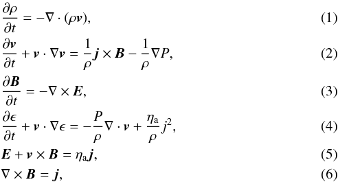$\begin{array}{ccc}& & \\ & & \\ & & \\ & & \\ & & \\ & & \end{array}$using the Lare2d code (Arber et al. 2001), with normalising scales given by and 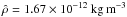. The choice of is reflective of the coronal environment (Priest 2014), while is similar to that used in other simulations of magnetic reconnection (e.g. Gordovskyy et al. 2010). The lengthscale is chosen to be comparable to the current sheet size, which is not well constrained for the solar corona; current sheet sizes similar to ours have been used (see e.g. Litvinenko 1996; Wood & Neukirch 2005), however so have much larger ones (e.g. Kliem 1994; Gordovskyy et al. 2010). This choice of lengthscale pushes the limits of the applicability of MHD within the solar corona, however it was used in order to achieve a compromise between the use of self-consistent electromagnetic fields (from the MHD simulation) while at the same time incorporating aspects of microscopic physics into the particle acceleration picture (without the use of kinetic simulations). In the absence of scattering, test particle energies scale with the square of length, meaning that orbit calculations performed with a given choice of lengthscale can be extrapolated by simply adjusting the energies appropriately. This is not generally the case with scattering included, as the mean free path associated with the scattering introduces a scale independent of the MHD lengthscale which impacts the particle orbits. Increasing the lengthscale substantially, without changing the scattering mean free path, would result in particle orbit computation becoming prohibitively computationally expensive. Although it would be possible to circumvent this issue by, for example, restricting the domain size within which particle orbit calculations are performed, doing so would restrict the effect of the geometrical configuration of the MHD fields on the particle simulation. The normalising scales for all other parameters come from combinations of and and are quoted in Table 1. We set the anomalous resistivity (η_a) to zero where the critical current is below a threshold value of j_crit = 1, while η_a = 10^-4 where the current exceeds j_crit (values of j_crit and η_a are given in normalised units).

Our simulation of 2D magnetic reconnection starts with an isothermal force-free Harris sheet whose magnetic field is perturbed in order to initiate reconnection. The equations specifying the initial conditions for the MHD simulation are given in Eqs. (7)–(10):

$\begin{array}{ccc}& & \frac{{\mathit{B}}_{\mathit{x}}}{\mathit{B̂}}\mathrm{=}\tanh \mathrm{\left(}\mathit{y}\mathrm{\right)}\mathrm{-}\frac{{\mathit{b}}_{\mathrm{1}}}{{\mathit{b}}_{\mathrm{0}}}{\mathit{k}}_{\mathit{y}}\cos \mathrm{\left(}{\mathit{k}}_{\mathit{x}}\mathit{x}\mathrm{\right)}\sin \mathrm{\left(}{\mathit{k}}_{\mathit{y}}\mathit{y}\mathrm{\right)}\mathit{,}\\ & & \frac{{\mathit{B}}_{\mathit{y}}}{\mathit{B̂}}\mathrm{=}\frac{{\mathit{b}}_{\mathrm{1}}}{{\mathit{b}}_{\mathrm{0}}}{\mathit{k}}_{\mathit{x}}\cos \mathrm{\left(}{\mathit{k}}_{\mathit{y}}\mathit{y}\mathrm{\right)}\sin \mathrm{\left(}{\mathit{k}}_{\mathit{x}}\mathit{x}\mathrm{\right)}\mathit{,}\\ & & \frac{{\mathit{B}}_{\mathit{z}}}{\mathit{B̂}}\mathrm{=}\mathrm{sech}\mathrm{\left(}\mathit{y}\mathrm{\right)}\mathit{,}\\ & & \frac{\mathit{\epsilon }}{\mathit{\epsilon ̂}}\mathrm{=}\frac{{\mathit{T}}_{\mathrm{0}}\mathit{/}\mathit{T̂}}{{\mathit{m}}_{\mathrm{r}}\mathrm{(}{\mathit{\gamma }}_{\mathrm{p}}\mathrm{-}\mathrm{1}\mathrm{)}}\mathit{,}\end{array}$

where b₁/b₀ = 0.3, T₀ = 10⁶ K, m_r = 1.2 is the reduced mass for coronal plasma normalised to the proton mass, and γ_p = 5 / 3 is the ratio of specific heats. We specify the initial density to be uniform at a value of . Our domain has size 15 in the x-direction and 60 in the y-direction so that our choices of k_x = 2π/ 15, k_y = 2π/ 60 ensure the perturbation has one period within the domain in both directions. Periodic boundary conditions in the x-direction and closed boundary conditions in the y-direction are imposed. The magnetic field corresponding to the initial conditions is shown in Fig. 1a.

We evolve the MHD simulation until the reconnection rate drops to near-zero and we use an individual snapshot from the simulation (shown in Fig. 1b) during the reconnecting phase into which we insert test particles to compute particle orbits. For simplicity we pick a single MHD snapshot as the electromagnetic field structure changes on a longer timescale than the particle evolution. We shall see in Sect. 4.3 that the majority of the particle orbits’ durations are less than 0.1 ms and the MHD fields do not vary a great deal during the main reconnection phase which lasts approximately 1 ms (this can be seen from the evolution of the magnetic energy in Fig. 1d, which steadily decreases between 1 and 2 ms).

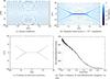Fig. 1 Magnetic field lines (black) and out of plane electric field (colour) for a) the initial conditions of the MHD simulation, and b) the chosen snapshot into which test particles are injected. We present only the subset of the MHD simulation domain which is within the test particle computational box. Panel c: areas where current density exceeds the threshold value for triggering anomalous resistivity and coincides with the region where scattering takes place. Panel d: evolution of the magnetic energy in the simulation, with the red star indicating the time at which the snapshot used for the particle simulation is taken.

3. Governing equations for test particle evolution

Charged particle evolution is governed by the Lorentz force law, dv/ dt = q⁽E + v × B⁾, which can, in principle, be solved numerically for the trajectory of the particle. Unfortunately the timestep required to resolve the evolution of the test particle is too small to be practical (for the magnetic field strengths typical of the corona). A common alternative is to use the guiding centre approximation when computing particle orbits (see for example Gordovskyy et al. 2010; Threlfall et al. 2016; Borissov et al. 2016). In this approach the position of the test particle is averaged over a gyration period (this averaged position is referred to as the guiding centre). This method allows the use of longer timesteps, because the particle gyration need not be resolved temporally. The equations for the evolution of the guiding centre in prescribed electromagnetic fields are given by Northrop (1963) and are reproduced in Eqs. (11), (12):

$\begin{array}{ccc}& & \dot{{R}}\mathrm{\perp }\mathrm{=}\frac{{b}}{\mathit{B}}\mathrm{\times }[\mathrm{-}{E}\mathrm{+}\frac{\mathit{\mu }}{\mathit{\gamma e}}\mathrm{\nabla }\mathit{B}\mathrm{+}\frac{\mathit{mU}}{\mathit{e}}\frac{\mathrm{d}{b}}{\mathrm{d}\mathit{t}}\mathrm{+}\frac{\mathit{m\gamma }}{\mathit{e}}\frac{\mathrm{d}{{u}}_{\mathit{E}}}{\mathrm{d}\mathit{t}}\\ & & \mathrm{+}\hspace{0.17em}\frac{\mathit{U}}{\mathit{\gamma }}{\mathit{E}}_{\mathrm{\parallel }}{{u}}_{\mathit{E}}\mathrm{+}\frac{\mathit{\mu }}{\mathit{\gamma e}}{{u}}_{\mathit{E}}\frac{\mathit{\partial B}}{\mathit{\partial t}}]\mathit{,}\\ & & \mathit{m}\frac{\mathrm{d}\mathit{U}}{\mathrm{d}\mathit{t}}\mathrm{=}\mathit{m\gamma }{{u}}_{\mathit{E}}\mathrm{·}\frac{\mathrm{d}{b}}{\mathrm{d}\mathit{t}}\mathrm{+}\mathit{e}{\mathit{E}}_{\mathrm{\parallel }}\mathrm{-}\frac{\mathit{\mu }}{\mathit{\gamma }}\frac{\mathit{\partial B}}{\mathit{\partial s}}\mathit{,}\end{array}$

where the Lorentz factor, γ, is given by: $\mathit{\gamma }\mathrm{=}\sqrt{\mathrm{1}\mathrm{+}\frac{{\mathit{U}}^{\mathrm{2}}\mathrm{+}{\mathit{u}}_{\mathit{E}}^{\mathrm{2}}}{{\mathit{c}}^{\mathrm{2}}}\mathrm{+}\frac{\mathrm{2}\mathit{\mu B}}{\mathit{m}{\mathit{c}}^{\mathrm{2}}}}\mathrm{·}$(13)Here R denotes the guiding centre position, and $\dot{{R}}{}_{\mathrm{\perp }}$ is the drift velocity of the guiding centre perpendicular to the magnetic field. The E cross B drift of the guiding centre is given by u_E = γV_E = γE × B/B², U = γv_∥ = γv·b is the velocity of the guiding centre parallel to the magnetic field, and b is the unit vector in the direction of the magnetic field. The quantity ∂B/∂s is the rate of change of the magnetic field strength along the guiding centre trajectory. Finally, $\mathit{\mu }\mathrm{=}\mathit{m}{\mathit{\gamma }}^{\mathrm{2}}{\mathit{v}}_{\mathrm{\perp }}^{\mathrm{2}}\mathit{/}\mathrm{\left(}\mathrm{2}\mathit{B}\mathrm{\right)}$ is the magnetic moment, v_⊥ = v_totsinθ is the gyrational component of the total particle velocity, v_tot = |v|, m is the electron mass, and e the electron charge. The guiding centre approach is valid as long as the length and timescales on which the underlying fields vary are large compared with the particle gyroradius and gyroperiod. In our simulations the maximum value of the ratio of the electron gyroradius to the width of the current sheet is approximately 0.03, while the maximum value of the ratio of the electron gyroperiod to the MHD timescale is 0.007, justifying our use of the guiding centre model. We use the relativistic version of the guiding centre equations even though the particle energies we obtain are generally non-relativistic.

In regions where η_a = 0 we solve Eqs. (11)–(13) with an adaptive timestep 4th order Runge Kutta scheme. The guiding centre equations conserve the magnetic moment along the particle trajectory, which cannot be true if pitch angle scattering occurs. By modifying the magnetic moment, along with self-consistently modifying U, we can introduce pitch angle scattering into the governing equations of particle motion. To account for pitch angle scattering in regions where η_a ≠ 0, in addition to solving Eqs. (11), (12) we also solve: $\begin{array}{ccc}\mathrm{d}\mathit{\gamma }& \mathrm{=}& \mathit{\gamma ̇}\mathrm{d}\mathit{t,}\\ \mathrm{d}\mathit{\beta }& \mathrm{=}& \mathrm{(}\mathit{\beta ̇}\mathrm{+}{\mathit{F}}_{\mathit{\beta }}\mathrm{)}\mathrm{d}\mathit{t}\mathrm{+}\sqrt{\mathrm{2}{\mathit{D}}_{\mathit{\beta \beta }}}\mathrm{d}\mathit{W,}\end{array}$where β = cosθ, and d$\mathit{W}\mathrm{=}\mathit{\zeta }\sqrt{\mathrm{d}\mathit{t}}$ and ζ is a normally distributed random variable. Expressions for and are given by:

$\begin{array}{ccc}& & \mathit{\gamma ̇}\mathrm{=}\frac{\mathrm{1}}{\mathrm{2}}{\left(\mathrm{1}\mathrm{+}\frac{{\mathit{U}}^{\mathrm{2}}}{{\mathit{c}}^{\mathrm{2}}}\mathrm{+}\frac{\mathrm{2}\mathit{\mu B}}{\mathit{m}{\mathit{c}}^{\mathrm{2}}}\right)}^{\mathrm{-}\mathrm{1}\mathit{/}\mathrm{2}}\left(\frac{\mathrm{2}\mathit{U}}{{\mathit{c}}^{\mathrm{2}}}\frac{\mathrm{d}\mathit{U}}{\mathrm{d}\mathit{t}}\mathrm{+}\frac{\mathrm{2}\mathit{\mu }}{\mathit{m}{\mathit{c}}^{\mathrm{2}}}\frac{\mathrm{d}\mathit{B}}{\mathrm{d}\mathit{t}}\right){\left(\mathrm{1}\mathrm{-}\frac{{\mathit{V}}_{\mathit{E}}^{\mathrm{2}}}{{\mathit{c}}^{\mathrm{2}}}\right)}^{\mathrm{-}\mathrm{1}\mathit{/}\mathrm{2}}\mathit{,}\\ & & \mathit{\beta ̇}\mathrm{=}\left(\frac{\mathrm{1}}{\mathit{U}}\frac{\mathrm{d}\mathit{U}}{\mathrm{d}\mathit{t}}\mathrm{-}\frac{\mathrm{1}}{\mathrm{2}\mathit{B}}\frac{\mathrm{d}\mathit{B}}{\mathrm{d}\mathit{t}}\right)\mathit{\beta }\mathrm{(}\mathrm{1}\mathrm{-}{\mathit{\beta }}^{\mathrm{2}}\mathrm{)}\mathit{.}\end{array}$

Equations (16) and (17) follow from taking time derivatives of the expressions for γ and μ (see appendix for derivation). Although Eq. (14) may be replaced by simply updating the energy through the definition of the Lorentz factor in the guiding centre equations (Eq. (13)), this approach was implemented in order to allow generalisation of the scattering model in future work. Our initial choice of the friction and diffusion coefficients F_β and D_ββ are F_β = − βv_tot/λ and D_ββ = (1 − β²)v_tot/λ, where the mean free path is parametrised by 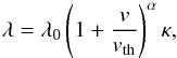$\mathit{\lambda }\mathrm{=}{\mathit{\lambda }}_{\mathrm{0}}{\left(\mathrm{1}\mathrm{+}\frac{\mathit{v}}{{\mathit{v}}_{\mathrm{th}}}\right)}^{\mathit{\alpha }}\mathit{\kappa ,}$(18)with λ₀ = 2 × 10⁸ m, representing the mean free path of an electron in a plasma with coronal parameters. We integrate Eqs. (14) and (15) using an Euler scheme whose timestep is the minimum of dt₀ = 5 × 10^-9 s and dt_s = 1 / (3ν) = λ/ (3v_tot). The value for dt₀ was determined by comparing results of integrating particle trajectories between the variable timestep code (without scattering) and imposing F_β = D_ββ = 0 with the fixed timestep code. Multiple values of dt₀ were evaluated and one was chosen that could accurately reproduce the trajectory given by the variable timestep code. Although a higher order scheme would have been preferable, the dependence of the coefficients on the particle position in the grid would necessitate extra computation of spatial gradients of the fields, which would increase computation time. Furthermore the timestep must be less than the time between scattering events, hence requiring the choice of the minimum of dt₀ and dt_s. After updating β and γ, we update the magnetic moment and parallel velocity to calculate the position of the guiding centre in Eq. (11). The position is then integrated by the Runge-Kutta scheme with the timestep used in the Euler scheme, dt₀.

4. Results of test particle calculations

4.1. Configuration of test particle code

To study the effect of pitch angle scattering on particle behaviour, we initialise test particle orbits in the MHD snapshot shown in Fig. 1b, and integrate the governing equations for their evolution, detailed in Sect. 3, until the orbit leaves the computational domain. We compare the results of calculations in the presence of different scattering rates by varying the values of κ and α in Eq. (18). The parameter α determines how the mean free path changes as a function of test particle velocity, with α> 0 resulting in a longer mean free path (and hence less scattering) at higher particle velocities, while α< 0 results in a decreasing mean free path for higher velocities. A simple scaling of the mean free path can be applied by varying κ, with higher values leading to a longer mean free path and less scattering. We introduce a dependence on the anomalous resistivity into the mean free path by setting κ = η_sp/η_a, where η_sp is the local Spitzer resistivity at the position of the guiding centre. To get an idea of the spatial dependence of the Spitzer resistivity on position in our MHD simulation, a contour plot of the ratio κ = η_sp/η_a is shown in Fig. 2.

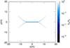Fig. 2 Spatial dependence of the ratio of Spitzer resistivity to anomalous resistivity in the snapshot of the MHD simulation into which test particles are injected. White areas surrounding the current sheet do not have a specified anomalous resistivity, hence the ratio is calculated only where ηa ≠ 0.

We perform test particle simulations with the following choices of parameters: to investigate the effect of velocity-dependent scattering we choose α = ± 2,0, with κ = η_sp/η_a; to investigate the effect of anomalous resistivity we take α = 0 and κ = 10^-5,10^-6,2 × 10^-8,η_sp/η_a. The mean free path is related to the scattering frequency by ν = v_tot/λ. In order for the guiding centre approximation to remain valid, the scattering frequency must not exceed the gyrofrequency of the test particle. This restriction on the scattering frequency is dependent on the test particle gyrational velocity, as well as the local magnetic field strength. It is difficult to predict if a test particle orbit will break this condition, however, we find that for values κ< 5 × 10^-9 the scattering frequency starts to regularly exceed the gyrofrequency. In addition to performing test particle simulations with scattering included at different rates, we perform the same simulations without scattering using the variable timestep 4th order Runge-Kutta code. We refer to these simulations as the control cases.

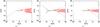Fig. 3 Orbit trajectories for test particles initialised at (x,y) = (0,0),(0,5) m (black and red trajectories respectively) within the MHD snapshot. The initial pitch angle is 90° and kinetic energy 320 eV. Test particle orbit calculations were performed a) without scattering, b) with scattering where κ = 10-6, and c) where κ = ηsp/ηa.

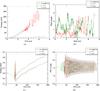Fig. 4 Orbit energy and pitch angle evolution for the trajectories calculated above. Panels a and b refer to orbits initialised within the current sheet (i.e. for y = 0 m), while panels c and d refer to orbits initialised outside of the current sheet (at y = 5 m).

To compute test particle energy spectra, we integrate 5 × 10⁵ particle orbits for each of the parameter regimes mentioned above. The particle orbits are distributed with uniformly random initial positions inside a portion of the computation box. This portion is centred on the reconnection region and has a side length of 2 in normalised units (the whole computational box has a side length of 4, also centred on the reconnection region; see Fig. 1b). The initial pitch angle takes on 100 evenly distributed values between 10° and 170° and the initial energy takes on 50 evenly distributed values between 10 eV and 320 eV (this energy range covers over 90% of the maxwellian at 10⁶ K). These choices mean that there are 100 particle orbits for every combination of initial pitch angle and energy, each having a different (uniformly random) initial position.

The final energy and position of each orbit is recorded as it exits the computational box. Each orbit is weighted in proportion to the plasma density at its initial position, so that the initial particle energy distribution is approximately a Maxwellian at a temperature of 10⁶ K and the initial distribution of the cosine of the pitch angle is uniform. The resulting energy spectra are shown in Fig. 5.

4.2. Selected trajectories

Our primary interests are the energy spectra obtained through many orbit calculations, however, it is initially enlightening to examine selected orbit trajectories, energy, and pitch angle evolution. Such examples reveal the general effect of pitch angle scattering on individual orbits. To do this we place test particles at two distinct initial positions, y₀ = 0 and 5 m (in both cases with x = 0 m), with initial pitch angle θ₀ = 90° and kinetic energy is 320 eV, into the MHD snapshot. These initial conditions are chosen so that the effect of scattering is evident on orbits that drifts into the reconnection region due to the E × B drift, as well as for orbits starting within the reconnection region. The particle trajectories are calculated as described in the previous Sect. with no scattering, scattering with κ = 10^-6 in Eq. (18), and with κ = η_sp/η_a. The resulting trajectories, energy evolution, and pitch angle evolution are shown in Figs. 3 and 4.

Due to the magnetic moment no longer being conserved in the case of the different scattering regimes, the orbit trajectories in Figs. 3b and c differ from the control case (Fig. 3a). This is caused by terms in the guiding centre equations (Eqs. (11), (12)) proportional to μ having a randomising effect on the particle drifts when scattering is included (as μ is no longer constant). For the particle orbit initialised in the current sheet, the more chaotic evolution of the pitch angle when κ = η_sp/η_a (see green curve in Fig. 4b in comparison to the red and black curves) suggests that this choice of κ produces stronger scattering within the diffusion region than if κ = 10^-6. When κ = 10^-6, we note that the particle orbit crosses the reconnection region multiple times (see black particle orbits in Figs. 3b and c), as has been reported previously (see Burge et al. 2014), which is an effect that cannot happen in the absence of scattering. Orbits which enter the current sheet multiple times can traverse a greater potential drop than if they were evolving deterministically, and hence gain more energy. Due to the stochastic nature of the orbit, such behaviour and associated increased energy is not guaranteed even with identical orbit initial conditions. We anticipate that the presence of scattering will yield energy spectra containing higher maximum energies than the case without scattering, as a result of particle trajectories traversing the reconnection region multiple times.

Orbits which start outside of the reconnection region are not subject to as much scattering and acceleration if they drift into the separatrices rather than the central current sheet. As a result, although some scattering is evident in the trajectory (red lines in Fig. 3) and pitch angle evolution (Fig. 4d) of the particle orbits initialised at y = 5 m, energy changes at the end of the orbit are much less evident than for the particle orbits initialised inside the current sheet.

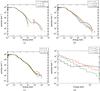Fig. 5 Final test particle energy spectra for various scattering models. In all cases 5 × 105 test particle orbits are calculated, then each orbit is weighted in proportion to the local density at the initial position of the orbit to ensure the initial energy distribution is a Maxwellian at T = 106 K, and that the initial pitch angle cosine distribution is uniform. Section 4.1 shows the initial conditions of the simulations. In panels a and b we set α = 0 and vary the value of κ, whereas in panel c we take κ = ηsp/ηa and vary α. Panel d shows the spectra from panel b between 1 and 100 keV.

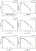Fig. 6 Panel a: histogram of the duration of the particle orbits for the simulations without scattering, and with scattering where κ = 2 × 10-8 and κ = ηsp/ηa. Panels b–f: spectra consisting of particle orbits with durations for the indicated time range.

4.3. Energy spectra

In Fig. 5a we compare the spectra produced by the control case (without scattering, black curve), with the scattering cases where κ = 10^-5,10^-6 (in both of these we set α = 0). We note that there is a break in the spectrum of the control case. A small population of highly accelerated particles achieve energies of approximately 100 keV (approximately 0.3% of the total number of orbits, after weighting). This break in the spectrum is due to the small size of the reconnection region. When scattering is introduced, with κ = 10^-5 (red curve in Fig. 5a), there is an increase in the spread of energies obtained by the highly energised particles orbits (compared to the control case), while the general shape of the spectrum remains unchanged. The spectrum of the scattering case with κ = 10^-6 (green curve in Fig. 5a) is smoother, without any breaks in the spectrum. This suggests that scattering is much more effective for smaller values of κ. Both green and red curves in Fig. 5a contain significant numbers of particle orbits achieving energies much greater than the maximum energy achieved by any particle orbit in the control case (in both scattering regimes approximately 0.15% of particle orbits achieve energies higher than any unscattered orbit, corresponding to approximately half of the total highly accelerated population in the control case).

Next we compare spectra produced with κ given by κ = η_sp/η_a to the constant κ = 10^-6 and κ = 2 × 10^-8 cases, again with α = 0 (see Fig. 5b). Figure 5d shows a restricted energy range (between 1 and 200 keV) of the same spectra. The value of κ = 2 × 10^-8 is chosen to be comparable to the minimum value of η_sp/η_a (since η_sp ∝ T^{− 3 / 2} this is the location in the MHD simulation with the highest temperature, i.e. in the middle of the current sheet). Since all three cases examined here include relatively strong scattering, we see that there are no breaks in any spectrum, and furthermore there are more particles with energies in the region of 10 keV in the case when κ = η_sp/η_a and κ = 2 × 10^-8 than when κ = 10^-6, with fewer higher energy particles (in particular 1.6% of the total particle orbits have energies between 5 and 30 keV for the case κ = η_sp/η_a, compared to 2.3% for the κ = 2 × 10^-8 case and 0.5% for the κ = 10^-6 case). The dependency of the mean free path on the resistivity leads to lower maximum energies than even a constant but lower value of κ. This is because the ratio η_sp/η_a increases drastically in the separatrices where the temperature is lower, resulting in fewer particles being scattered. The absence of scattering within the separatrices means that fewer orbits are able to repeatedly cross the acceleration region, resulting in lower energies. We also note that scattering with κ = 2 × 10^-8 yields fewer particles at energies above 100 keV when compared with the κ = 10^-6 case. In both cases, the maximum energy obtained by particles is still higher than for the case without scattering.

Finally, in Fig. 5c, we consider spectra produced by varying the velocity dependence of the scattering model. In Figs. 5a and b we fixed α = 0 and varied values of κ. Now we set κ = η_sp/η_a and consider α = − 2,0,2. There is a very small difference in the spectra above 1 keV, with the α = − 2 case having very slightly more particle orbits at lower energies (8.1% of total particle orbits with energies between 1 and 10 keV, as opposed to 7.9% and 7.6% for the α = 0 and α = 2 cases respectively) and fewer higher energy orbits (0.004% of total particle orbits with energies greater than 100 keV, as opposed to 0.01% and 0.04% for the α = 0 and α = 2 cases respectively). The spectrum for the α = 0 case falls in between the other two. This indicates stronger scattering occurring for large negative α. This is to be expected as the mean free path decreases for large ratios of the particle velocity to the thermal velocity, implying more scattering. The small difference between three values of α is due to the factor 1 + v_tot/v_th only varying between approximately 1 and 6 for a test particle starting at the centre of the dissipation region (where the temperature and electric field are at their maximum). Changing the mean free path by several orders of magnitude when varying κ has a much greater impact on the spectrum than a change in the velocity dependence.

The presence of pitch angle scattering should decrease the rate at which particles are accelerated. In Fig. 6a we plot a histogram of orbit durations in cases without scattering (black curve), with scattering where κ = 2 × 10^-8 (red curve) and κ = η_sp/η_a (green curve, in both of the scattering cases α = 0). We see that the number of particles per duration only varies between the three cases above 0.1 ms durations. The number of particle orbits with duration greater than 0.1 ms is about 14% for the no scattering case, rising to 16% for the scattering case where κ = η_sp/η_a and 22% when κ = 2 × 10^-8. Figures 6b−f show orbit spectra with successively longer durations. We note that the spectra of the simulations including scattering extend to progressively higher energies when particle orbits with progressively longer durations are considered. This is again due to particle orbits needing multiple traverses of the current sheet in order to gain energies higher than those possible in the absence of scattering. The abrupt step in the spectra in Figs. 6b−e at approximately 320 keV is due to the particle orbits which exit the computational box without having encountered the reconnection region. This happens relatively quickly (the exact orbit duration would depend on the initial pitch angle, position, and kinetic energy of each particle orbit, but in all cases occurs faster than 0.1 ms) and, as such, these particle orbits are not present in Fig. 6f, resulting in a much smoother spectrum. It is interesting to note the presence of a distinct shoulder starting at energies of approxmately 20 keV in Fig. 6f for the κ = η_sp/η_a spectrum. Given the already small number of particle orbits which last longer than 0.1 ms, it is not surprising that this feature is not seen in the full spectrum in Fig. 5b.

4.4. Particle orbit escape positions

We now turn our attention to the impact of scattering on the final positions of each test particle orbit upon exiting the computational box. In Fig. 7 we produce histograms for the final z and y positions. We do this for the scattering model when κ = η_sp/η_a (green curve) and κ = 2 × 10^-8 (red curve), in both cases with α = 0, in addition to the control case (black curve). In the control case the highly accelerated particle population primarily escapes the simulation domain between z = 200 and z = 300 m causing a prominent increase seen on the right hand side of Fig. 7a. In contrast, scattering results in more spread in the final z-position. The two scattering models differ in the distribution of the particle orbits final z-position, with scattering in the κ = η_sp/η_a model resulting in a narrower range of exit locations, compared to the stronger scattering case, with κ = 2 × 10^-8, seen in the broader red curve in Fig. 7a.

In Fig. 7b we present a histogram of the y-value at the point where the particles exit the computation box. The two tallest peaks correspond to the separatrices, with values between them corresponding to the reconnection outflow region. We see that the κ = η_sp/η_a scattering model and the control case give very similar results, with 14% and 12% of the total particle orbits exiting within the outflow region respectively. In the case of much stronger scattering with κ = 2 × 10^-8 , significantly more orbits exit within the outflow region (20% of total). Stronger scattering in the separatrices (in the case of the κ = 2 × 10^-8 case) causes more particle orbits to be scattered from the separatrices into the outflow region. Since no scattering takes place in this region and the E × B drift is directed outward, the test particles are unable to re-enter the current sheet and exit the simulation box in the outflow region. For higher values of κ, or for κ = η_sp/η_a, scattering is much weaker in the separatrices, resulting in a distribution of final y-values much closer to that of the control case.

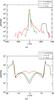Fig. 7 Histograms of the y-, and z-positions of particle orbit escape from computational box in the absence of scattering and for the κ = 2 × 10-8 and κ = ηsp/ηa scattering regimes. In both scattering cases, α is set to zero.

5. Discussion and conclusions

We have presented a very simple model of pitch angle scattering and have shown that it can have a significant impact on test particle energy spectra. In previous studies which included the effects of collisional scattering (e.g. Numata & Yoshida 2002; Burge et al. 2014), it was found that repeated crossings of the reconnection region by test particles in the presence of scattering could lead to a higher energy gain than in the absence of scattering, but that the effect on energy spectra was not significant. In our work, the strong dependence of the mean free path on the anomalous resistivity is the main aspect of the model which affects the energy spectra and box escape positions. Due to this strong scattering, the spectra we obtain show a significant number of orbits gaining energies higher than is possible without scattering, which is something that is not seen in Burge et al. (2014), probably due to their use of a much lower scattering rate.

If we interpret κ from Eq. (18) as the dependence of the mean free path on the anomalous resistivity, the difference between constant and spatially varying (κ = η_sp/η_a) values of κ are mainly due to their behaviour in regions away from the central current sheet. Since our MHD simulations involved a constant anomalous resistivity where the current exceeded a specified threshold, whereas the Spitzer resistivity calculated at the location of the guiding centre is dependent on temperature, our choice of κ = η_sp/η_a resulted in the scattering rate decreasing with temperature (this is a result of η_sp ∝ T^{− 3 / 2}). The weaker scattering in the separatrices due to the lower temperature (in comparison to the temperature inside the central current sheet) impacted the dynamics of the particles. Less scattering in the separatrices resulted in fewer orbits re-entering the current sheet multiple times. Therefore, the temperatures calculated in the MHD simulations have a significant effect on the test particle dynamics and energy spectra. The temperatures achieved in our MHD simulations are somewhat unrealistic, with a maximum temperature of 4.2 × 10⁹ K, due to the lack of thermal conduction or radiation used. This resulted in the small values of η_sp/η_a ≈ 10^-8 in the current sheet. In future work this could be remedied by the inclusion of thermal conduction and radiation in the MHD simulation. On the other hand, Bian et al. (2016) showed that thermal conduction can be significantly reduced in coronal conditions due to pitch angle scattering, leading to temperatures of the order of 10⁸ K. The reduced thermal conductivity means it is reasonable that there is a large difference in temperature between the current sheet and the separatrices, resulting in a correspondingly large difference in the scattering rates and the associated test particle dynamics. We also showed that there are some small differences between an increasing and decreasing mean free path dependence as a function of the total test particle velocity, however they were negligible in comparison to the changes to the spectra as a result of varying κ.

The guiding centre formalism we used relies on the test particle being able to complete at least one full gyration in order to define a guiding centre, so the scattering rate is limited by the gyrofrequency. Our choice of scattering model, in particular κ = η_sp/η_a, would result in violating this restriction for values of anomalous resistivity more than an order of magnitude greater than the ones chosen. This may be remedied by solving full particle orbits for the time that the test particle is within the diffusion region (as in Burge et al. 2014). On the other hand, a further decrease in the anomalous resistivity in the MHD simulations would require a greater resolution, which would eventually take prohibitively long amounts of time to compute.

In contrast to previous work on particle acceleration in 2D reconnection (for instance in Gordovskyy et al. 2010), the maximum energies achieved in our simulations are relatively small (of the order of 100 keV). This is a result of our use of a relatively small lengthscale causing small electric field strengths and size of reconnection region. For a given test particle orbit, the energy gain is entirely dependent on the electric potential drop that it traverses, with possible additional energy losses due to scattering. The presence of scattering introduces an additional lengthscale, namely the mean free path, which means that it is no longer possible to scale the resulting energy spectra with the MHD lengthscale. Our model of scattering did not include any energy loss during collisions, hence changes in the energy spectra are purely due to the different trajectories that particles take and the potential drop that they encounter along it. The inclusion of energy loss terms can be easily accommodated by adding stochastic terms to the energy evolution equation (Eq. (14)). This may result in an optimal anomalous resistivity for the acceleration of charged particles.

Finally, more complicated magnetic field topologies are likely to impact the results obtained in this paper with regards to particle trajectories and possibly energy spectra. It would be worth investigating how test particle acceleration is modified in 3D reconnection configurations such as that studied in Threlfall et al. (2016) or in coronal structures such as a flux tube (see e.g. Gordovskyy et al. 2014) with the addition of anomalous scattering.

Acknowledgments

A.B. would like to thank the University of St Andrews for financial support from the 7th Century Scholarship and the Scottish Government for support from the Saltire Scholarship. E.P.K.’s work is partially supported by a STFC consolidated grant ST/L000741/1. J.T. and T.N. gratefully acknowledge the support of the UK STFC (consolidated grant SN/N000609/1).

References

Appendix A: Calculating and

Since the guiding centre approach does not involve the total particle velocity, instead of the usual definition of the Lorentz factor we use, $\begin{array}{ccc}{\mathit{\gamma }}^{\mathrm{2}}& \mathrm{=}& \mathrm{1}\mathrm{+}\frac{{\mathit{\gamma }}^{\mathrm{2}}{\mathit{v}}^{\mathrm{2}}}{{\mathit{c}}^{\mathrm{2}}}\\ & \mathrm{\simeq }& \mathrm{1}\mathrm{+}\frac{{\mathit{U}}^{\mathrm{2}}}{{\mathit{c}}^{\mathrm{2}}}\mathrm{+}\frac{\mathrm{2}\mathit{\mu B}}{\mathit{m}{\mathit{c}}^{\mathrm{2}}}\mathrm{+}\frac{{\mathit{\gamma }}^{\mathrm{2}}{\mathit{V}}_{\mathit{E}}^{\mathrm{2}}}{{\mathit{c}}^{\mathrm{2}}}\\ & \mathrm{=}& \frac{\mathrm{1}\mathrm{+}\frac{{\mathit{U}}^{\mathrm{2}}}{{\mathit{c}}^{\mathrm{2}}}\mathrm{+}\frac{\mathrm{2}\mathit{\mu B}}{\mathit{m}{\mathit{c}}^{\mathrm{2}}}}{\mathrm{1}\mathrm{-}\frac{{\mathit{V}}_{\mathit{E}}^{\mathrm{2}}}{{\mathit{c}}^{\mathrm{2}}}}\mathit{,}\end{array}$where we used the fact that the E × B is the dominant guiding centre drift. Therefore, $\mathit{\gamma }\mathrm{=}\frac{\sqrt{\mathrm{1}\mathrm{+}\frac{{\mathit{U}}^{\mathrm{2}}}{{\mathit{c}}^{\mathrm{2}}}\mathrm{+}\frac{\mathrm{2}\mathit{\mu B}}{\mathit{m}{\mathit{c}}^{\mathrm{2}}}}}{\sqrt{\mathrm{1}\mathrm{-}\frac{{\mathit{V}}_{\mathit{E}}^{\mathrm{2}}}{{\mathit{c}}^{\mathrm{2}}}}}\mathrm{·}$(A.1)Differentiating this with respect to time yields, $\begin{array}{ccc}\mathit{\gamma ̇}& \mathrm{=}& \frac{\mathrm{1}}{\mathrm{2}}{\left(\mathrm{1}\mathrm{+}\frac{{\mathit{U}}^{\mathrm{2}}}{{\mathit{c}}^{\mathrm{2}}}\mathrm{+}\frac{\mathrm{2}\mathit{\mu B}}{\mathit{m}{\mathit{c}}^{\mathrm{2}}}\right)}^{\mathrm{-}\mathrm{1}\mathit{/}\mathrm{2}}\left(\frac{\mathrm{2}\mathit{U}}{{\mathit{c}}^{\mathrm{2}}}\frac{\mathrm{d}\mathit{U}}{\mathrm{d}\mathit{t}}\mathrm{+}\frac{\mathrm{2}\mathit{\mu }}{\mathit{m}{\mathit{c}}^{\mathrm{2}}}\frac{\mathrm{d}\mathit{B}}{\mathrm{d}\mathit{t}}\right){\left(\mathrm{1}\mathrm{-}\frac{{\mathit{V}}_{\mathit{E}}^{\mathrm{2}}}{{\mathit{c}}^{\mathrm{2}}}\right)}^{\mathrm{-}\mathrm{1}\mathit{/}\mathrm{2}}\\ & & \mathrm{+}\frac{\mathrm{1}}{\mathrm{2}}{\left(\mathrm{1}\mathrm{-}\frac{{\mathit{V}}_{\mathit{E}}^{\mathrm{2}}}{{\mathit{c}}^{\mathrm{2}}}\right)}^{\mathrm{-}\mathrm{3}\mathit{/}\mathrm{2}}{\left(\mathrm{1}\mathrm{+}\frac{{\mathit{U}}^{\mathrm{2}}}{{\mathit{c}}^{\mathrm{2}}}\mathrm{+}\frac{\mathrm{2}\mathit{\mu B}}{\mathit{m}{\mathit{c}}^{\mathrm{2}}}\right)}^{\mathrm{1}\mathit{/}\mathrm{2}}\frac{\mathrm{2}{\mathit{V}}_{\mathit{E}}}{{\mathit{c}}^{\mathrm{2}}}\frac{\mathrm{d}{\mathit{V}}_{\mathit{E}}}{\mathrm{d}\mathit{t}}\mathrm{·}\end{array}$(A.2)Since V_E ≪ c, the second term is negligible in comparison to the first term, resulting in Eq. (16).

For β = cosθ the derivation of the time derivative, is much more straightforward. Since $\mathit{\mu }\mathrm{=}\frac{\mathit{m}{\mathit{u}}^{\mathrm{2}}{\mathit{\beta }}^{\mathrm{2}}}{\mathrm{2}\mathit{B}}\mathrm{=}\frac{\mathit{m}{\mathit{U}}^{\mathrm{2}}}{\mathrm{2}\mathit{B}}\frac{\mathrm{1}\mathrm{-}{\mathit{\beta }}^{\mathrm{2}}}{{\mathit{\beta }}^{\mathrm{2}}}$ and $\frac{\mathrm{d}\mathit{\mu }}{\mathrm{d}\mathit{t}}\mathrm{=}\mathrm{0}$ we have: $\begin{array}{ccc}\mathrm{0}\mathrm{=}\frac{\mathrm{d}\mathit{\mu }}{\mathrm{d}\mathit{t}}& \mathrm{=}& \frac{\mathit{mU}}{\mathit{B}}\frac{\mathrm{1}\mathrm{-}{\mathit{\beta }}^{\mathrm{2}}}{{\mathit{\beta }}^{\mathrm{2}}}\frac{\mathrm{d}\mathit{U}}{\mathrm{d}\mathit{t}}\mathrm{+}\frac{\mathit{m}{\mathit{U}}^{\mathrm{2}}\mathit{\beta }}{\mathit{B}}\left(\mathrm{-}\frac{\mathrm{2}}{{\mathit{\beta }}^{\mathrm{3}}}\right)\frac{\mathrm{d}\mathit{\beta }}{\mathrm{d}\mathit{t}}\mathrm{-}\frac{\mathit{m}{\mathit{U}}^{\mathrm{2}}}{\mathrm{2}{\mathit{B}}^{\mathrm{2}}}\frac{\mathrm{1}\mathrm{-}{\mathit{\beta }}^{\mathrm{2}}}{{\mathit{\beta }}^{\mathrm{2}}}\frac{\mathrm{d}\mathit{B}}{\mathrm{d}\mathit{t}}\\ & \mathrm{=}& \frac{\mathrm{2}\mathit{\mu }}{\mathit{U}}\frac{\mathrm{d}\mathit{U}}{\mathrm{d}\mathit{t}}\mathrm{-}\frac{\mathrm{2}\mathit{\mu }}{\mathit{\beta }\left(\mathrm{1}\mathrm{-}{\mathit{\beta }}^{\mathrm{2}}\right)}\frac{\mathrm{d}\mathit{\beta }}{\mathrm{d}\mathit{t}}\mathrm{-}\frac{\mathit{\mu }}{\mathit{B}}\frac{\mathrm{d}\mathit{B}}{\mathrm{d}\mathit{t}}\mathrm{·}\end{array}$Therefore, the time derivative, , can be expressed as: $\mathit{\beta ̇}\mathrm{=}\left(\frac{\mathrm{1}}{\mathit{U}}\frac{\mathrm{d}\mathit{U}}{\mathrm{d}\mathit{t}}\mathrm{-}\frac{\mathrm{1}}{\mathrm{2}\mathit{B}}\frac{\mathrm{d}\mathit{B}}{\mathrm{d}\mathit{t}}\right)\mathit{\beta }\mathrm{(}\mathrm{1}\mathrm{-}{\mathit{\beta }}^{\mathrm{2}}\mathrm{)}\mathit{.}$(A.3)

All Tables

All Figures

Fig. 1 Magnetic field lines (black) and out of plane electric field (colour) for a) the initial conditions of the MHD simulation, and b) the chosen snapshot into which test particles are injected. We present only the subset of the MHD simulation domain which is within the test particle computational box. Panel c: areas where current density exceeds the threshold value for triggering anomalous resistivity and coincides with the region where scattering takes place. Panel d: evolution of the magnetic energy in the simulation, with the red star indicating the time at which the snapshot used for the particle simulation is taken.

In the text

	Fig. 2 Spatial dependence of the ratio of Spitzer resistivity to anomalous resistivity in the snapshot of the MHD simulation into which test particles are injected. White areas surrounding the current sheet do not have a specified anomalous resistivity, hence the ratio is calculated only where ηa ≠ 0.
In the text

	Fig. 3 Orbit trajectories for test particles initialised at (x,y) = (0,0),(0,5) m (black and red trajectories respectively) within the MHD snapshot. The initial pitch angle is 90° and kinetic energy 320 eV. Test particle orbit calculations were performed a) without scattering, b) with scattering where κ = 10-6, and c) where κ = ηsp/ηa.
In the text

	Fig. 4 Orbit energy and pitch angle evolution for the trajectories calculated above. Panels a and b refer to orbits initialised within the current sheet (i.e. for y = 0 m), while panels c and d refer to orbits initialised outside of the current sheet (at y = 5 m).
In the text

Fig. 5 Final test particle energy spectra for various scattering models. In all cases 5 × 105 test particle orbits are calculated, then each orbit is weighted in proportion to the local density at the initial position of the orbit to ensure the initial energy distribution is a Maxwellian at T = 106 K, and that the initial pitch angle cosine distribution is uniform. Section 4.1 shows the initial conditions of the simulations. In panels a and b we set α = 0 and vary the value of κ, whereas in panel c we take κ = ηsp/ηa and vary α. Panel d shows the spectra from panel b between 1 and 100 keV.

In the text

	Fig. 6 Panel a: histogram of the duration of the particle orbits for the simulations without scattering, and with scattering where κ = 2 × 10-8 and κ = ηsp/ηa. Panels b–f: spectra consisting of particle orbits with durations for the indicated time range.
In the text

	Fig. 7 Histograms of the y-, and z-positions of particle orbit escape from computational box in the absence of scattering and for the κ = 2 × 10-8 and κ = ηsp/ηa scattering regimes. In both scattering cases, α is set to zero.
In the text

References

- Arber, T., Longbottom, A., Gerrard, C., & Milne, A. 2001, J. Comput. Phys., 171, 151 [NASA ADS] [CrossRef] [Google Scholar]
- Benz, A. O. 2008, Liv. Rev. Sol. Phys., 5, 1 [Google Scholar]
- Bian, N. H., Kontar, E. P., & Emslie, A. G. 2016, ApJ, 824, 78 [NASA ADS] [CrossRef] [Google Scholar]
- Bian, N. H., Emslie, A. G., & Kontar, E. P. 2017, ApJ, 835, 262 [NASA ADS] [CrossRef] [Google Scholar]
- Birn, J., & Priest, E. R. 2007, Reconnection of Magnetic Fields (UK: Cambridge University Press) [Google Scholar]
- Borissov, A., Neukirch, T., & Threlfall, J. 2016, Sol. Phys., 291, 1385 [NASA ADS] [CrossRef] [Google Scholar]
- Burge, C. A., MacKinnon, A. L., & Petkaki, P. 2014, A&A, 561, A107 [NASA ADS] [CrossRef] [EDP Sciences] [Google Scholar]
- Cargill, P. J., Vlahos, L., Baumann, G., Drake, J. F., & Nordlund, Å. 2012, Space Sci. Rev., 173, 223 [NASA ADS] [CrossRef] [Google Scholar]
- Gordovskyy, M., Browning, P. K., & Vekstein, G. E. 2010, A&A, 519, A21 [NASA ADS] [CrossRef] [EDP Sciences] [Google Scholar]
- Gordovskyy, M., Browning, P. K., Kontar, E. P., & Bian, N. H. 2013, Sol. Phys., 284, 489 [NASA ADS] [CrossRef] [Google Scholar]
- Gordovskyy, M., Browning, P. K., Kontar, E. P., & Bian, N. H. 2014, A&A, 561, A72 [NASA ADS] [CrossRef] [EDP Sciences] [Google Scholar]
- Jeffrey, N. L. S., Kontar, E. P., Bian, N. H., & Emslie, A. G. 2014, ApJ, 787, 86 [NASA ADS] [CrossRef] [Google Scholar]
- Kliem, B. 1994, ApJS, 90, 719 [NASA ADS] [CrossRef] [Google Scholar]
- Kontar, E. P., Bian, N. H., Emslie, A. G., & Vilmer, N. 2014, ApJ, 780, 176 [NASA ADS] [CrossRef] [Google Scholar]
- Kontar, E. P., Perez, J. E., Harra, L. K., et al. 2017, Phys. Rev. Lett., 118, 155101 [NASA ADS] [CrossRef] [Google Scholar]
- Litvinenko, Y. E. 1996, ApJ, 462, 997 [NASA ADS] [CrossRef] [Google Scholar]
- Northrop, T. G. 1963, The Adiabatic Motion of Charged Particles (New York: John Wiley & Sons, Inc.) [Google Scholar]
- Numata, R., & Yoshida, Z. 2002, Phys. Rev. Lett., 88, 045003 [NASA ADS] [CrossRef] [Google Scholar]
- Papadopoulos, K. 1977, Rev. Geophys. Space Phys., 15, 113 [NASA ADS] [CrossRef] [Google Scholar]
- Petrosian, V. 2012, Space Sci. Rev., 173, 535 [NASA ADS] [CrossRef] [Google Scholar]
- Priest, E. 2014, Magnetohydrodynamics of the Sun (Cambridge, UK: Cambridge University Press) [Google Scholar]
- Priest, E. R., & Forbes, T. G. 2002, A&ARv, 10, 313 [NASA ADS] [CrossRef] [Google Scholar]
- Shibata, K., & Magara, T. 2011, Liv. Rev. Sol. Phys., 8, 6 [Google Scholar]
- Threlfall, J., Stevenson, J. E. H., Parnell, C. E., & Neukirch, T. 2016, A&A, 585, A95 [NASA ADS] [CrossRef] [EDP Sciences] [Google Scholar]
- Treumann, R. A. 2001, Earth, Planets, and Space, 53, 453 [Google Scholar]
- Treumann, R. A., & Baumjohann, W. 2015, A&ARv, 23, 4 [NASA ADS] [CrossRef] [Google Scholar]
- Wood, P., & Neukirch, T. 2005, Sol. Phys., 226, 73 [NASA ADS] [CrossRef] [Google Scholar]
- Zharkova, V. V., Arzner, K., Benz, A. O., et al. 2011, Space Sci. Rev., 159, 357 [NASA ADS] [CrossRef] [Google Scholar]