© ESO, 2017

1. Introduction

Magnetic fields are expected to play a key role in the physics of high-density molecular clouds. For instance, strong magnetic fields may support clouds against gravitational collapse and thus prevent or delay star formation (e.g., Crutcher 2007; Li et al. 2014). An intense magnetic field also influences the dynamics of the first evolutionary stages of a Sun-like (proto-)star and its (proto-)planetary systems (e.g., Königl & Ruden 1993; Frank et al. 2014). In particular, if closely coupled with the infalling gas, the magnetic field can be an efficient tool to disperse the angular momentum, possibly preventing the development of an accretion disk (Hennebelle & Fromang 2008). Finally, strong disk-like magnetic fields could have implication for planet formation and migration (Bai & Stone 2013). Therefore, the study of magnetic fields provides a valuable opportunity to shed further light on the formation and evolution of interstellar clouds as well as on star formation. The Zeeman effect is the only means by which magnetic field strengths can be measured in interstellar clouds (e.g., Crutcher et al. 1993). However, interstellar Zeeman observations are strongly hampered by the weakness of the effect. Furthermore, most of the common interstellar molecules are closed-shell species (i.e., non-paramagnetic species) and, therefore, they do not show easy to measure Zeeman effect.

Focusing on emissions due to molecules associated with star forming regions, the first successful attempt to detect the Zeeman effect was made for OH absorptions toward the NGC 2024 molecular cloud (Crutcher & Kazés 1983). Only later on, Zeeman detections were extended to CN molecular lines (Crutcher et al. 1999), whereas attempts for other species have not resulted in any definite detections. Thus, to the best of our knowledge, the Zeeman effect has been unambiguously detected in non-masing interstellar gas only in OH and CN lines, whereas it has been detected in OH, CH₃OH, SiO, and H₂O intense masers (Crutcher 2012). These findings call for laboratory studies to characterize the Zeeman effect in further molecular species. Very few radicals are known to possess the three attributes required to have an observable effect (see Uchida et al. 2001): (i) large g factors, (ii) high critical densities, and (iii) bright line emission. Sulfur monoxide (SO), a ${}^{\mathrm{3}}\mathrm{\Sigma }_{\mathit{g}}^{\mathrm{-}}$ radical in its ground electronic state, meets these three requirements. In addition, SO is a very abundant species in almost all the components associated with the star forming regions, from dark clouds to protostellar envelopes and outflows, as well as hot corinos (e.g., van Dishoeck & Blake 1998).

Bel & Leroy (1989) calculated the Zeeman splitting due to a longitudinal magnetic field for some transitions of diatomic molecules, showing that for OH, CN, and SO this effect might be detectable as soon as the magnetic field is of the order of 100 μG. Successively, SO was chosen by Uchida et al. (2001) to study the dense gas in dark clouds and high-mass star forming regions: the authors used the N,J = 2, 1 ← 1, 1 line profiles (at ~13 GHz) observed with the MPIfR Effelsberg 100-m antenna. However, only upper limits on the magnetic field strength were obtained.

The first laboratory spectroscopic study of SO dates back to Martin (1932); since then, many works have been dedicated to the rotational and vibrational analysis of its ground and excited electronic states, including isotopically substituted species; we refer to Martin-Drumel et al. (2015), Lattanzi et al. (2015), and references therein. Fewer studies have been devoted to a detailed Zeeman analysis of this radical. The first characterization of the Zeeman effect in SO was reported by Winnewisser et al. (1964), while Daniels & Dorain (1966) derived the g values of the electron spin (g_s), the orbital (g_l), and the rotational magnetic moments (g_r) of SO by means of Electron Paramagnetic Resonance (EPR) measurements. More than ten years later, Kawaguchi et al. (1979) carried out laser magnetic resonance spectroscopy experiments for SO in the electronic ground state with a CO₂ laser as source, leading to the determination of the g factors for both the vibrational ground and first excited state. Finally, calculated Zeeman splittings for some SO lines between 30 and 179 GHz were reported by Shinnaga & Yamamoto (2000). However, the most thorough analysis of the g factors prior to this work was performed by Christensen & Veseth (1978), who determined the g factors for the ground states of O₂ and SO by means of a weighted nonlinear least-squares fit including zero-field as well as Zeeman data. The experimental determination of Christensen & Veseth (1978) was supported by single-determinant LCAO-wave function computations (LCAO stands for Linear Combination of Atomic Orbitals), with relativistic corrections to g’s arising from the reduction of the Breit equation to the second Pauli limit, also considered.

The goal of the present work is twofold: (i) to obtain an accurate characterization of the Zeeman effect in SO by means of laboratory work and theoretical studies; and (ii) to identify rotational transitions that show the strongest effect in the (sub-)millimeter spectral regions, covered by new-generation interferometers such as IRAM-NOEMA and ALMA. In the following sections, the details of the experimental apparatus are described. Subsequently, the theoretical background to analyze the Zeeman effect as well as the details of our quantum-chemical computations are presented. Finally, the results are reported and possible astrophysical implications are discussed.

2. Experimental details

Measurements were carried out with a frequency modulated, computer-controlled spectrometer (65 GHz−1.6 THz), described in detail in Cazzoli & Puzzarini (2006, 2013), Puzzarini et al. (2012). The Zeeman effect was produced by applying a magnetic field parallel to the radiation propagation. A solenoid, which results from three overlapped wrappings of copper wire (1 mm diameter), is wrapped coaxially around the cell (a glass tube ~2 m long). A direct current (DC) voltage is applied to the solenoid in order to produce a current that can be varied linearly from about 0.2 to 15 A (producing a magnetic field of 2.3 G to 170.2 G) and kept fixed during the measurements. The solenoid is 1.5 m long and contains 903 turns/m. This piece of information was used to derive an initial estimate of the magnitude of the magnetic field (in Gauss) generated by the total current I_tot (in amperes): 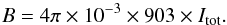$\mathit{B}\mathrm{=}\mathrm{4}\mathit{\pi }\mathrm{\times }{\mathrm{10}}^{-3}\mathrm{\times }\mathrm{903}\mathrm{\times }{\mathit{I}}_{\mathrm{tot}}\mathit{.}$(1)Subsequently, a calibration was performed thereby exploiting the Zeeman effect in O₂ (${}^{\mathrm{3}}\mathrm{\Sigma }^{\mathrm{-}}$), thus leading to a correction factor of 0.98196(4) to be applied to the magnetic field resulting from Eq. (1). To cancel the Zeeman effect due to the terrestrial magnetic field, a small magnetic field was applied perpendicularly to the cell. The calibration was carried out without the parallel magnetic field and the most sensitive transitions were used. The Zeeman effect in molecular oxygen was considered for two reasons: the accurate experimental g_s and g_l values from Christensen & Veseth (1978) and g_r from Evenson & Mizushima (1972) were employed to calibrate (as explained in the following) our experimental set up as well as to benchmark our computational results.

Samples of SO were prepared directly inside the absorption cell employing a flow of ~30 mTorr of O₂ and a DC discharge of 12 mA, at room temperature. The use of H₂S and of other sulfur-bearing chemicals in previous unrelated experiments led to sulfur being adsorbed on cell walls and thus allowed us to achieve good signals of SO without further addition of S-containing compounds (Lattanzi et al. 2015). For O₂ measurements, a commercial sample was used instead. Since the O₂ transitions are weak (because their intensity only depends on its molecular magnetic moment), measurements were performed at the liquid nitrogen temperature, thus obtaining in this way a good signal-to-noise ratio (S/N).

A preliminary investigation of the Zeeman effect was carried out by considering 19 transitions selected in the 86−844 GHz frequency range. The detailed list is given in Table 1, where the first column reports the unperturbed transition frequency, the second one the lower state energy (E_low), and the last the quantum numbers involved.

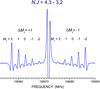Fig. 1 N,J = 4, 3 ← 3, 2 transition of SO at 159.0 GHz: Zeeman spectrum obtained by applying a magnetic field of 22.3 G.

For all of them, the overall Zeeman spectra were recorded. These showed different Zeeman effects in terms of magnitude and shape, as illustrated in Figs. 1 to 4. Only the seven transitions that showed the strongest effect and a good S/N were further considered, namely:

• N,J = 2, 2 ← 1, 1 at at 86.1 GHz;

• N,J = 4, 3 ← 3, 2 at 159.0 GHz (see Fig. 1);

• N,J = 1, 1 ← 0, 1 at 286.3 GHz;

• N,J = 2, 2 ← 1, 2 at 309.5 GHz (see Fig. 2);

• N,J = 2, 1 ← 1, 0 at 329.4 GHz;

• N,J = 9, 8 ← 8, 7 at 384.5 GHz (see Fig. 3);

• N,J = 9, 10 ← 8, 9 at 389.1 GHz (see Fig. 4).

For four of them, illustrative pictures are reported (Figs. 1−4): they have been chosen to provide an overview on how Zeeman spectra can be different. Furthermore, as mentioned above, to calibrate the magnetic field apparatus (see Eq. (1)), three rotational transitions of O₂ (${}^{\mathrm{3}}\mathrm{\Sigma }^{\mathrm{-}}$) were investigated: that is, the 368.5 GHz (N,J = 3, 2 ← 1, 1), 424.8 GHz (N,J = 3, 2 ← 1, 2; Fig. 5), and 487.2 GHz (N,J = 3, 3 ← 1, 2) transitions. For molecular oxygen, the g factors required for the calibration were taken from Evenson & Mizushima (1972) and Christensen & Veseth (1978).

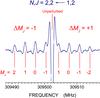Fig. 2 N,J = 2, 2 ← 1, 2 transition of SO at 309.5 GHz: Zeeman spectrum obtained by applying a magnetic field of 11.2 G.

Fig. 3 N,J = 9, 8 ← 8, 7 transition of SO at 384.5 GHz: Zeeman spectrum obtained by applying a magnetic field of 111.4 G (in blue); the calculated stick spectrum (in red) is also depicted. In the inset, an example of a single recording is shown.

As evident from Figs. 1 to 4, the Zeeman effect produces a splitting of the transition in several Zeeman components due to the removal of the degeneracy of the (2J + 1) magnetic components (more details in the following section). To measure the frequency of the Zeeman components to the best possible accuracy, the most important condition is that the applied magnetic field remains constant during the measurement. To fulfill such a requirement, each component was measured separately (an example is provided by the inset of Fig. 3). During the measurement, the solenoid current was kept constant by means of a computer-controlled power supply and measured at each step of the spectrum recording process; the mean value was subsequently used in the analysis. The current was found to be stable during the measurement, with a standard deviation of the order of 10^-4 A. The accuracy of our measurements was set to range from 30 kHz to 100 kHz, mostly depending on the S/N (Landman et al. 1982; Cazzoli et al. 2004).

3. Computational and theoretical details

3.1. Zeeman effect

For SO, the total angular momentum J results from the coupling of the rotational angular momentum N, the electronic angular momentum L, and the spin angular momentum S. Since the electronic ground state of SO is a ${}^{\mathrm{3}}\mathrm{\Sigma }_{\mathit{g}}^{\mathrm{-}}$ state, the quantum number associated with the component of the electronic angular momentum along the internuclear axis (Λ) is zero, and the effective Hamiltonian operator can be expressed in terms of the quantum numbers J and N corresponding to the total angular momentum J and the rotational angular momentum N, respectively. For a given value of N, the quantum number J can assume three possible values: N−1, N, and N + 1, with the condition that J should be greater than zero.

When a magnetic field is applied, the degeneracy of the projection of the total angular momentum along the direction of the applied field is removed, as made evident in Figs. 1 and 2. As a result, for a given value of J, the rotational level is split into 2J + 1 components: M_J = +J, +(J−1), ..., 0, ..., −J.

To obtain the corresponding energy, for each M_J value, the energy matrix, built for N ranging from 0 to 50, has been diagonalized. The non-zero elements of this matrix are:$\begin{array}{ccc}\mathit{J}& \mathrm{=}& \mathit{N}\mathrm{+}\mathrm{1}\mathrm{:}\mathrm{⟨}\mathit{J,}{\mathit{M}}_{\mathrm{J}}\mathrm{\left|}\mathit{Ĥ}\mathrm{Z}\mathrm{\right|}\mathit{J,}{\mathit{M}}_{\mathrm{J}}\mathrm{⟩}\mathrm{=}{\mathit{\mu }}_{\mathrm{B}}{\mathit{B}}_{\mathrm{Z}}{\mathit{M}}_{\mathrm{J}}\left[\frac{{\mathit{g}}_{\mathrm{s}}}{\mathrm{(}\mathit{N}\mathrm{+}\mathrm{1}\mathrm{)}}\mathrm{+}\mathrm{2}\frac{{\mathit{g}}_{\mathrm{l}}}{\mathrm{(}\mathrm{2}\mathit{N}\mathrm{+}\mathrm{3}\mathrm{)}}\right]\\ \mathit{J}& \mathrm{=}& \mathit{N}\mathrm{:}\mathrm{⟨}\mathit{J,}{\mathit{M}}_{\mathrm{J}}\mathrm{\left|}\mathit{Ĥ}\mathrm{Z}\mathrm{\right|}\mathit{J,}{\mathit{M}}_{\mathrm{J}}\mathrm{⟩}\mathrm{=}{\mathit{\mu }}_{\mathrm{B}}{\mathit{B}}_{\mathrm{Z}}{\mathit{M}}_{\mathrm{J}}\left[\frac{{\mathit{g}}_{\mathrm{s}}}{\mathit{N}\mathrm{(}\mathit{N}\mathrm{+}\mathrm{1}\mathrm{)}}\mathrm{-}{\mathit{g}}_{\mathrm{r}}\right]\\ \mathit{J}& \mathrm{=}& \mathit{N}\mathrm{-}\mathrm{1}\mathrm{:}\mathrm{⟨}\mathit{J,}{\mathit{M}}_{\mathrm{J}}\mathrm{\left|}\mathit{Ĥ}\mathrm{Z}\mathrm{\right|}\mathit{J,}{\mathit{M}}_{\mathrm{J}}\mathrm{⟩}\mathrm{=}\mathrm{-}{\mathit{\mu }}_{\mathrm{B}}{\mathit{B}}_{\mathrm{Z}}{\mathit{M}}_{\mathrm{J}}\left[\frac{{\mathit{g}}_{\mathrm{s}}}{\mathit{N}}\mathrm{+}\mathrm{2}\frac{{\mathit{g}}_{\mathrm{l}}}{\mathrm{(}\mathrm{2}\mathit{N}\mathrm{-}\mathrm{1}\mathrm{)}}\right]\\ \mathit{J}& \mathrm{=}& \mathit{N}\mathrm{+}\mathrm{1}\mathrm{:}\mathrm{⟨}\mathit{J,}{\mathit{M}}_{\mathrm{J}}\mathrm{\left|}\mathit{Ĥ}\mathrm{Z}\mathrm{\right|}\mathit{J}\mathrm{-}\mathrm{1}\mathit{,}{\mathit{M}}_{\mathrm{J}}\mathrm{⟩}\mathrm{=}{\mathit{\mu }}_{\mathrm{B}}{\mathit{B}}_{\mathrm{Z}}\sqrt{\mathit{N}\mathrm{\left[}\mathrm{\right(}\mathit{N}\mathrm{+}\mathrm{1}{\mathrm{)}}^{\mathrm{2}}\mathrm{-}{\mathit{M}}_{\mathrm{J}}^{\mathrm{2}}\mathrm{]}}\\ & & \mathrm{\times }\left[\frac{{\mathit{g}}_{\mathrm{s}}}{\sqrt{\mathrm{(}\mathit{N}\mathrm{+}\mathrm{1}{\mathrm{)}}^{\mathrm{2}}\mathrm{(}\mathrm{2}\mathit{N}\mathrm{+}\mathrm{1}\mathrm{)}}}\mathrm{+}\frac{{\mathit{g}}_{\mathrm{l}}}{\sqrt{\mathrm{\left[}\mathrm{4}\mathrm{\right(}\mathit{N}\mathrm{+}\mathrm{1}{\mathrm{)}}^{\mathrm{2}}\mathrm{-}\mathrm{1}\mathrm{\left]}\mathrm{\right(}\mathrm{2}\mathit{N}\mathrm{+}\mathrm{3}\mathrm{)}}}\hspace{0.17em}\right]\\ \mathit{J}& \mathrm{=}& \mathit{N}\mathrm{:}\mathrm{⟨}\mathit{J,}{\mathit{M}}_{\mathrm{J}}\mathrm{\left|}\mathit{Ĥ}\mathrm{Z}\mathrm{\right|}\mathit{J}\mathrm{-}\mathrm{1}\mathit{,}{\mathit{M}}_{\mathrm{J}}\mathrm{⟩}\mathrm{=}{\mathit{\mu }}_{\mathrm{B}}{\mathit{B}}_{\mathrm{Z}}\sqrt{\mathrm{(}{\mathit{N}}^{\mathrm{2}}\mathrm{-}{\mathit{M}}_{\mathrm{J}}^{\mathrm{2}}\mathrm{)}\mathrm{(}\mathit{N}\mathrm{+}\mathrm{1}\mathrm{)}}\\ & & \mathrm{\times }\left[\frac{{\mathit{g}}_{\mathrm{s}}}{\sqrt{{\mathit{N}}^{\mathrm{2}}\mathrm{(}\mathrm{2}\mathit{N}\mathrm{+}\mathrm{1}\mathrm{)}}}\mathrm{+}\frac{{\mathit{g}}_{\mathrm{l}}}{\sqrt{\mathrm{(}\mathrm{4}{\mathit{N}}^{\mathrm{2}}\mathrm{-}\mathrm{1}\mathrm{)}\mathrm{(}\mathrm{2}\mathit{N}\mathrm{-}\mathrm{1}\mathrm{)}}}\hspace{0.17em}\right]\mathit{,}\end{array}$(2)where μ_B is the Bohr magneton, and B_Z the applied magnetic field along the Z axis. Ĥ_Z is the Zeeman part of the effective Hamiltonian (see, for example, Carrington et al. 1967; Christensen & Veseth 1978): $\mathit{Ĥ}\mathrm{Z}\mathrm{=}{\mathit{g}}_{\mathrm{s}}{\mathit{\mu }}_{\mathrm{B}}{B}\mathrm{·}{S}\mathrm{+}{\mathit{g}}_{\mathrm{l}}{\mathit{\mu }}_{\mathrm{B}}{B}\mathrm{·}{L}\mathrm{-}{\mathit{g}}_{\mathrm{r}}{\mathit{\mu }}_{\mathrm{B}}{B}\mathrm{·}{N}\mathit{.}$(3)To the energy levels obtained in this way, the selection rule ΔM_J = ± 1 (due to perpendicularity of the magnetic field applied to the oscillating magnetic field of the radiation) has been applied in order to derive the corresponding Zeeman shifts. Figures 3 and 4 show examples of the stick spectra that can be generated. The procedure above has been implemented in a computer code that allows the derivation of the g_s, g_l, and g_r factors (see Sect. 3.2) by means of a least-squares fit of the calculated Zeeman shifts to those experimentally determined.

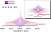Fig. 4 N,J = 9, 10 ← 8, 9 transition of SO at 389.1 GHz: experimental (in blue) and calculated (in red) Zeeman spectrum obtained by applying a magnetic field of 67 G.

3.2. Electronic and rotational g-tensors

To support the experimental determination of the g factors of SO, a systematic computational investigation of the latter for both SO and O₂ has also been carried out at the Coupled-Cluster (CC; Shavitt & Bartlett 2009) and Multiconfigurational Complete Active Space Self-Consistent-Field (CASSCF; Roos et al. 1980; Helgaker et al. 2000) levels of theory. The theoretical evaluation of the g_s and g_l factors requires the calculation of the electronic g-tensor. Briefly, the electronic g-tensor parametrizes the couplings between the external magnetic field B and the electronic spin S of the molecular system in Zeeman-effect-based spectroscopies and can be expressed in terms of a second-rank tensor 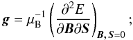${g}\mathrm{=}{\mathit{\mu }}_{\mathrm{B}}^{-1}{\left(\frac{{\mathit{\partial }}^{\mathrm{2}}\mathit{E}}{\mathit{\partial }{B}\mathit{\partial }{S}}\right)}_{{B,}\hspace{0.17em}{S}\mathrm{=}\mathrm{0}}\mathrm{;}$(4)The electronic g-tensor is typically written as: ${g}\mathrm{=}{\mathit{g}}_{\mathrm{e}}{1}\mathrm{+}\mathrm{\Delta }{g}\mathrm{\equiv }{\mathit{g}}_{\mathrm{e}}{1}\mathrm{+}\mathrm{\Delta }{{g}}_{\mathrm{pso}}\mathrm{+}\mathrm{\Delta }{{g}}_{\mathrm{dso}}\mathrm{+}\mathrm{\Delta }{{g}}_{\mathrm{rmc}}\mathit{,}$(5)where g_e is the free electron g factor (=2.002319304386(20), Mills et al. 1993). As indicated above, to determine the shift Δg three contributions are required: the so-called paramagnetic spin-orbit (pso) term (Δg_pso), the diamagnetic spin-orbit (dso) contribution (Δg_dso), and the term accounting for the relativistic mass corrections (rmc) (Δg_rmc). The paramagnetic spin-orbit term is a true second-order term, and involves orbital Zeeman and Spin-Orbit Coupling (SOC) operators (Harriman 1987; Engström et al. 1998; Kaupp et al. 2004). The other two contributions in Δg can be computed as expectation values of, respectively, the diamagnetic-spin orbit and kinetic energy operators, using the spin-density matrix in the latter case. The diamagnetic terms are also known under the name of one- and two-electron gauge contributions to the g tensor. Explicit expressions for the various terms are given in the literature (Harriman 1987; Engström et al. 1998; Kaupp et al. 2004) and will not be repeated here. We underline nonetheless that the two-electron SOC operator as well as the two-electron dso operator are often replaced by effective one-electron operators involving scaled nuclear charges (Koseki et al. 1995, 1998; Neese 2001) or based on a mean-field treatment (Hess et al. 1996; Neese 2005; Epifanovsky et al. 2015).

For linear molecules, the Δg_xx = Δg_yy components of the electronic g tensor are denoted as Δg_⊥, while Δg_zz is the parallel component Δg_∥. These are related to the measurable g factors by the following expressions: $\begin{array}{ccc}{\mathit{g}}_{\mathrm{s}}& \mathrm{=}& {\mathit{g}}_{\mathrm{\parallel }}\mathrm{=}{\mathit{g}}_{\mathrm{e}}\mathrm{+}\mathrm{\Delta }{\mathit{g}}_{\mathrm{\parallel }}\mathit{,}\\ {\mathit{g}}_{\mathrm{l}}& \mathrm{=}& \mathrm{\Delta }{\mathit{g}}_{\mathrm{\perp }}\mathit{.}\end{array}$Moreover, for a linear molecule in a Σ state the second-order contributions to the parallel component vanish.

The formalism adopted in this study to obtain the electronic g tensors at the CC level is thoroughly described in Gauss et al. (2009), as implemented in the CFOUR (Stanton et al. 2016) quantum chemistry suite of programs. The actual calculations employed an unrestricted Hartree-Fock (UHF) reference and were carried out with the center of mass chosen as gauge origin and with orbital relaxation effects included in the CC response treatment. At the CASSCF level, we employed the linear-response methodology of Vahtras et al. (1997, 2002), Engström et al. (1998), as implemented in the Dalton program package (Aidas et al. 2014). At the CC level only the scaled form of the SOC and dso operators was used, whereas both the full two-electron and the scaled one-electron operators were employed at the CASSCF level.

The rotational g-tensor parametrizes the energy difference between rotational levels due to the coupling between external magnetic field B and rotational angular momentum N$\mathrm{\Delta }\mathit{E}\mathrm{=}\mathrm{-}\frac{{\mathit{\mu }}_{\mathrm{n}}}{ħ}{{B}}^{\mathrm{T}}\mathrm{·}{{{g}}^{{\prime }}}_{\mathrm{r}}\mathrm{·}{N}\mathit{,}$(8)and thus it can be evaluated in terms of second derivatives of the energy with respect to the rotational angular momentum N and the external magnetic field B as perturbations (Gauss et al. 1996) $\begin{array}{ccc}{{{g}}^{{\prime }}}_{\mathrm{r}}\mathrm{=}\mathrm{-}ħ{\mathit{\mu }}_{\mathrm{n}}^{-1}{\left(\frac{{\mathit{\partial }}^{\mathrm{2}}\mathit{E}}{\mathit{\partial }{B}\mathit{\partial }{N}}\right)}_{{B,N}\mathrm{=}\mathrm{0}}\mathit{,}& & \end{array}$(9)where μ_n is the nuclear magneton. For a diatomic molecule, the rotational g-tensor has only two equivalent nonzero elements: ${\mathit{g}}_{\mathrm{r}}^{\mathrm{\prime }}\mathrm{=}{\mathit{g}}_{\mathit{xx}}\mathrm{=}{\mathit{g}}_{\mathit{yy}}\mathit{,}$(10)expressed in (m/M) units (with M and m being the proton and electron mass, respectively). To be compared with experiments (g_r), the calculated ${\mathit{g}}_{\mathrm{r}}^{\mathrm{\prime }}$ needs to be divided by the M/m ratio: ${\mathit{g}}_{\mathrm{r}}\mathrm{=}{\mathit{g}}_{\mathrm{r}}^{\mathrm{\prime }}\mathit{/}\mathrm{(}\mathit{M}\mathit{/}\mathit{m}\mathrm{)}\mathrm{=}{\mathit{g}}_{\mathrm{r}}^{\mathrm{\prime }}\mathit{/}\mathrm{1836.15267389}\mathrm{\left(}\mathrm{17}\mathrm{\right)}\mathit{.}$(11)For the calculation of the rotational g factor we followed the methodology presented in Gauss et al. (1996), Gauss et al. (2007).

The CC singles and doubles (CCSD; Purvis III & Bartlett 1982) and the CCSD with perturbative triples corrections (CCSD(T); Raghavachari et al. 1989) methods were adopted at the CC level. At the CASSCF level we considered for each molecule two different active spaces. For O₂, the active space labeled CAS1 in Table 2 consists of 12 electrons in 13 orbitals, whereas the CAS2 space includes 12 electrons in 14 orbitals. For SO (Table 3), CAS1 contains 10 electrons in 8 orbitals, and CAS2 space 10 electrons in 13 orbitals. We quantified the amount of multiconfigurational character of the wave function by analyzing the magnitude of the double excitation amplitudes in the CCSD calculations, and the coefficient of the leading determinant in the CASSCF calculation. The latter was greater than 0.95 for both species, and no large double excitation amplitudes were found in the CC treatment, indicating a modest multi-configurational character in both cases (at the geometry used in the calculations).

Different augmented correlation-consistent basis sets (Woon & Dunning 1993, 1995) were also considered in order to monitor the convergence of our results with respect to the one-electron space. Calculations for SO were carried out at two different geometries, namely the experimental equilibrium geometry and a computationally derived one. An optimized geometry was used for O₂. For both SO and O₂, the equilibrium structure was obtained by resorting to a composite scheme (Heckert et al. 2005, 2006) that accounts for extrapolation to the complete basis-set limit (CBS), core correlation (core) and the full treatment of triple (fT) and quadruple (fQ) excitations (CCSD(T)/CBS+CV+fT+fQ r_e).

Vibrational corrections were obtained using a discrete-variable representation (DVR) scheme with a quasi-analytic treatment of the kinetic energy (Vázquez et al. 2011) with 13 grid points and 13 harmonic-oscillator basis functions in the diagonalization step. The required potential curves have been determined at the fc-CCSD(T)/cc-pVTZ level, while the property values have been evaluated at the CCSD(T)/aug-pCVTZ level in the case of the electronic g-tensors and at the fc-CCSD(T)/aug-cc-pVTZ level in the case of the rotational g-tensor, respectively.

4. Results

Before discussing the experimental results, it is important to address the accuracy and reliability of our computed g factors. They are given in Tables 2 and 3 for O₂ and SO, respectively. It is necessary to discuss three issues here, namely, (a) basis-set convergence in the computations; (b) the accuracy of the CASSCF and the CC schemes; (c) and the reliability of the scaled Hamiltonian used in the CC computations.

Concerning the basis-set convergence, we note that convergence is fast for Δg_∥ and somewhat slower for Δg_⊥, but in all cases the values computed with the largest basis sets can be considered accurate within a few percent. The same observation also holds for g_r. The basis-set convergence for all g values seems to be slightly faster for O₂ than SO, but this is expected, since basis-set requirements are more demanding for third-row elements.

Considering the electron-correlation treatment, we note that the CASSCF and CC computations, despite their entirely different ansätze, provide rather similar results, in particular when we compare the CAS2 and CCSD(T) results (computed with the scaled Hamiltonian). The discrepancy between them, however, is somewhat larger than the estimated basis-set error and amounts, in the case of SO, to up to 10% for Δg_∥ and 5% for Δg_⊥ and g_r. The CCSD(T) results should be considered somewhat more accurate due to the more complete treatment of dynamical correlation and due to the fact that both O₂ and SO do not show particularly large static correlation effects that might render the CC treatment questionable. Finally, the use of a scaled Hamiltonian turns out to be problematic only in the case of Δg_∥. The reason is probably that for that term the paramagnetic contribution vanishes and that the scaling of the DSO terms is less rigorous. However, this has little consequence, as the Δg_∥ contribution is significantly smaller than Δg_⊥. For the latter component, the use of scaled charges only leads to a slight overestimation of the computed values (within 1 to 2%). Best theoretical estimates for the g factors are therefore most likely obtained by correcting the CCSD(T) values for the use of the scaled Hamiltonian, that is, a factor that is obtained from a comparison of the scaled and rigorous CAS2 computations (best estimates are collected in Table 4). As mentioned in the computational-detail section, corrections to account for zero-point vibrational effects have been evaluated (see Tables 2 and 3) and incorporated in the best theoretical values reported in Table 4. As noted in Tables 2 and 3, these corrections are small and almost negligible. Concerning the accuracy of the theoretical values, one furthermore needs to keep in mind that our computations do not go beyond CCSD(T), thus ignoring the effect of higher excitations. However, frozen-core CC singles, doubles, triples, quadruples (CCSDTQ) computations with the aug-cc-pVDZ basis set indicate that the contributions of quadruple excitations are of the order of ~1% for the perpendicular component of the electronic g-tensor and significantly less than 1% for the parallel component.

The last comment concerns the use of the computed g factors for the prediction of the Zeeman spectra. In this respect, Fig. 4 provides a significant example: the computed Zeeman spectrum (in red) is compared with the experimental one (in blue). A nearly perfect agreement is noted. This outcome thus opens up the possibility to accurately compute Zeeman spectra.

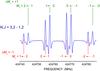Fig. 5 N,J = 3, 2 ← 1, 2 transition of O2 at 424.8 GHz: Zeeman spectrum obtained by applying a magnetic field of 5.7 G.

As mentioned above, molecular oxygen was used to calibrate the magnetic field applied. A total of 155 Zeeman components (for the three transitions considered) was measured, with the magnetic field varied from B = 2.3 G (I_tot = 0.2 Amp) to B = 113.5 G (I_tot = 10 Amp). Figure 5 shows the Zeeman spectrum for the N,J = 3, 2 ← 1, 2 transition when a magnetic field of 5.7 G is applied. The fit was carried out with the program described in the previous section, with the spectroscopic parameters and g factors fixed at the values of Yu et al. (2012) and Christensen & Veseth (1978), Evenson & Mizushima (1972), respectively; the only free parameter was the correction factor to be applied to the theoretical magnetic field (see Eq. (1)). The fit reproduces in a satisfactory manner the measured Zeeman components, with a standard deviation of 73 kHz (the uncertainty for the measured frequencies was in most cases set to 70 kHz). Moving to SO, for the seven transitions considered, a total of 353 Zeeman components were measured, with the magnetic field varied from B = 5.7 Gauss (I_tot = 0.5 Amp) to B = 124.8 Gauss (I_tot = 11 Amp), and fitted as described above. In the fitting procedure the spectroscopic parameters (i.e., the rotational, centrifugal distortion, and fine structure constants) were kept fixed at the values derived by Lattanzi et al. (2015). The g factors resulting from the fit are given in Table 4 together with the best-estimated values discussed above, while the complete set of the measured Zeeman components is available in the Supplementary Material. Alternative fits were carried out: In the first fit, the three g factors, g_s, g_l, and g_r, were fitted. In a second step, three different fits were carried out by fixing one of the three g factors and fitting the other two. In the last fit, only g_s was determined. We note that in the first fit, based on the comparison with theory, the g_s value is overestimated and the g_l value is underestimated; the two terms therefore seem to be correlated. For this reason, we performed the additional fits described above. We note that in all cases, g_r is determined with a limited accuracy, that is, with a relative uncertainty of ~20%. We also note that, if we fix g_s at the best computed value, a g_l value in good agreement with theory is obtained. However, by fixing g_l at the best estimate, the resulting g_s is still slightly overestimated. Simulations using values of g_s in the 2.0020−2.0030 range show that the Zeeman splittings only change by a few tens of kHz, that is, in most cases within the typical uncertainty affecting the frequency measurements. The last comment concerns the standard deviation of the fits that, in all cases, is about 50 kHz.

In Christensen & Veseth (1978) accurate values for the g factors were obtained (see Table 4). The g_s value is in perfect agreement with our best estimate, while g_l seems to be underestimated; the situation is different for g_r, which is largely overestimated with its value being more than three times larger than our computed value. A further comment on the results of Christensen & Veseth (1978) is merited. While for O₂ 214 high-precision data, including microwave and submillimeter-wave measurements as well as Laser Magnetic Resonance (LMR) and Electron Paramagnetic Resonance (EPR) data were used, for SO only 32 zero-field microwave frequencies together with 17 EPR observations were employed in the determination of the g factors. Despite the large set of data used for O₂, an unreliable value for g_r was obtained, thus suggesting a problem in the analysis for this term. However, this does not seem to affect the determination of g_s and g_l. For this reason, in the calibration of the experimental apparatus and in the benchmark study, the g_s and g_l values were taken from Christensen & Veseth (1978), while the g_r value derived by Evenson & Mizushima (1972) was used. It is also important to note that the g_s and g_l factors by Evenson & Mizushima (1972) were far less accurate and therefore not considered in the present work.

5. Astrophysical implications

Techniques based on the Zeeman effect are the only ones available for a direct measurement of the magnetic field strengths in interstellar clouds (Crutcher & Kazés 1983; Crutcher et al. 1993, 1999; Crutcher 2012). However, observation of the Zeeman effect turns out to be more complicated in space than in the laboratory. Because of light polarization, the intensities in terms of left-circularly polarized radiation (T_l), right-circularly polarized radiation (T_r), linearly polarized radiation parallel to B projected onto the Light of Sight (LoS) (T_∥), and linearly polarized radiation perpendicular to B projected onto the LoS (T_⊥) should be considered. In practice, the Stokes parameter I, V, Q, and U spectra need to be analyzed. In particular, I = T_∥ + T_⊥ and V = T_∥−T_⊥, which can also be rewritten as V = (dI/dν)cos θ, with Δν_Z being the shift in frequency due to the Zeeman effect, θ the angle between the LoS and the magnetic field and the effective Landé factor , given by (Landi Degl’Innocenti & Landolfi 2004): $\mathit{g̅}\mathrm{=}\frac{\mathrm{1}}{\mathrm{2}}\mathrm{(}{\mathit{g}}^{\mathit{up}}\mathrm{+}{\mathit{g}}^{\mathit{lo}}\mathrm{)}\mathrm{+}\frac{\mathrm{1}}{\mathrm{4}}\mathrm{(}{\mathit{g}}^{\mathit{up}}\mathrm{-}{\mathit{g}}^{\mathit{lo}}\mathrm{)}\mathrm{\left(}{\mathit{J}}^{\mathit{up}}\mathrm{\right(}{\mathit{J}}^{\mathit{up}}\mathrm{+}\mathrm{1}\mathrm{)}\mathrm{-}{\mathit{J}}^{\mathit{lo}}\mathrm{(}{\mathit{J}}^{\mathit{lo}}\mathrm{+}\mathrm{1}{\mathrm{\left)}}^{\mathrm{\right)}}\mathit{,}$(12)where up refers to the upper level and lo to the lower level of the transition. The g’s appearing in Eq. (12) are a combination of the g_s, g_l, and g_r values, according to Eqs. (2).

Stokes parameters Q and U are instead proportional to (d²I/dν²) and depend on θ, φ, which is the position angle of the component of B in the plane of the sky, and a second-order effective Landé factor, (see Landi Degl’Innocenti & Landolfi 2004), which is the equivalent for linear polarization of the factor used above in Stokes parameter V.

The overall result of the Zeeman effect is that the spectral line is split into three components, with a π component (ΔM_J = 0) unshifted in frequency and two σ components (ΔM_J = ± 1) shifted in frequency by Δν_Z = ± Z | B |, where Z is denoted as “Zeeman coefficient” and depends on the transition under consideration: $\mathrm{\left|}\mathrm{\Delta }{\mathit{\nu }}_{\mathrm{Z}}\mathrm{\right|}\mathrm{=}\mathrm{(}{\mathit{\mu }}_{\mathit{JN}}^{\mathit{up}}\mathrm{-}{{\mathit{\mu }}_{\mathit{JN}}^{\mathit{lo}}}^{\mathrm{)}}\mathrm{\left|}{B}\mathrm{\right|}\mathit{,}$(13)where, as above, up refers to the upper level and lo to the lower level. In turn, according to Uchida et al. (2001), μ_JN depends on the g factors as follows: ${\mathit{\mu }}_{\mathit{JN}}\mathrm{=}\mathrm{-}\frac{{\mathit{\mu }}_{\mathrm{B}}}{ħ}\left({\mathit{g}}_{\mathrm{s}}{S}\mathrm{+}{\mathit{g}}_{\mathrm{l}}{L}\right)\mathrm{+}\frac{{\mathit{\mu }}_{\mathrm{n}}}{ħ}\left({\mathit{g}}_{\mathrm{r}}{N}\right)\mathit{.}$(14)The coefficient Z can be used to identify the transitions showing the strongest Zeeman effect, which is observed when 2 × Z is approximately equal to μ_B, that is, equal to 1.40 Hz/μG (Crutcher 2012). It is therefore evident that Z depends on the quantum numbers, but not on the spectral-line frequency.

To experimentally determine Z for the transitions considered, the convoluted spectra of the ΔM_J = + 1 and ΔM_J = −1 components have been considered and their maxima have been used to evaluate the | Δν_Z | to be divided by the magnitude of the applied magnetic field. The values obtained are collected in Table 5 in terms of the Zeeman splitting (2Δν_Z/| B | = 2Z), and compared to previous results (Bel & Leroy 1989; Shinnaga & Yamamoto 2000). Table 5 also collects the Zeeman splittings for some of the transitions that were not investigated in detail. For them, the determination is less accurate because it is based on Zeeman spectra recorded for only one value of the magnetic field applied, while for the transitions studied in depth, Z resulted from recordings at different B values. From the analysis of Table 5, we note that the transitions at 159.0 GHz and 178.6 GHz were previously considered by Bel & Leroy (1989) and Shinnaga & Yamamoto (2000), respectively. For the former transition a reasonable agreement is observed, whereas for the other transition, our determination leads to a value about half of the one derived by Shinnaga & Yamamoto (2000). However, it should be pointed out that both works reported calculated values, while the present study is the first experimental determination. For comparison purposes, the Zeeman splittings for selected thermal transitions of CN, OH, and CCH (that show the strongest Zeeman effect) are collected in Table 5. We note that, even if somewhat less strong, SO exhibits effects comparable to that of CN, OH, and CCH. Obviously, intense masers (usually observed in H₂O, CH₃OH, and OH transitions emitting in the spectral cm-window) also provide the possibility to measure magnetic field strengths in the high-densities gas (up to 10¹¹ cm^-3) associated with high-mass star forming regions (e.g., Vlemmings 2007; Crutcher 2012,and references therein). Maser lines are characterized by narrow emissions (usually ≤1 km s-1), which are in principle suited to reveal the Zeeman effect. However, the analysis of polarized maser spectra is often hampered by complex small-scale spatial and velocity structures, and by a large number of blended lines, each of them with different polarization degrees.

Among the rotational transitions we investigated, those that show, in decreasing order, the largest Zeeman shifts are (i) N,J = 1, 1 ← 0, 1 at 286.3 GHz, (ii) N,J = 2, 2 ← 1, 2 at 309.5 GHz, (iii) N,J = 2, 1 ← 1, 0 at 329.4 GHz, (iv) N,J = 2, 2 ← 1, 1 at 86.1 GHz, and (v) N,J = 4, 3 ← 3, 2 at 159.0 GHz. For them, we derived the following values of Z: 0.87, 0.61, 0.53, 0.47, and 0.40 Hz/μG, respectively. Furthermore, from Table 5 it is evident that the N,J = 9, 8 ← 8, 7 (384.5 GHz) and N,J = 9 ,10 ← 8 ,9 (389.1 GHz) transitions, despite showing a strong Zeeman effect (see, Figs. 3 and 4), provide small Zeeman splittings. This is due to the fact that the most intense magnetic components are those closer to the unperturbed frequency.

In principle, when Δν_Z>δν, with δν being the observed full width at half maximun (FWHM) of the line, the complete set of information concerning the magnetic field B can be derived. However, for most of the Zeeman detections, the Zeeman splitting Δν_Z turns out to be significantly smaller than δν. Indeed, even if we neglect the non-thermal line broadening due to typical processes occurring in star forming regions such as jets (with velocities up to hundreds of km s^-1), outflows, and accreting/rotating disks (typically ≤10 km s^-1), already the thermal broadening (even at kinetical temperatures lower than 10 K) is definitely larger than the Zeeman splitting (e.g., Frank et al. 2014). For instance, a typical linewidth of the coldest starless cores is ~0.1 km s^-1 (e.g., di Francesco et al. 2007), indeed too broad to allow an observer to unveil the Zeeman effect. The expected B values in star forming regions range from ~100 μG, for low-mass objects (Li et al. 2014), to ~1 mG, as measured in regions hosting high-mass young stars (e.g., Pillai et al. 2016; Momjian & Sarma 2017). If we consider the N,J = 1, 1 ← 0, 1 transition (286.3 GHz), for which the largest Zeeman shift was obtained (Z = 0.87 Hz/μG), and we assume that B varies in the 0.1–1 mG range, we derive Δν_Z≃ values in the 87–870 Hz range, that is, 0.3–3 m s^-1. Moving to higher frequencies and considering the SO N,J = 2, 2 ← 1, 2 transition at 309.5 GHz, we derive Δν_Z ≃ 61−610 Hz, that is, 0.06−0.59 m s^-1. In conclusion, in such cases, only information about the LoS component of B, B_∥, is obtained. In fact, the Stokes parameter Q and U spectra are usually too weak to be detected. The analysis is therefore limited to the Stokes V spectrum, which has the shape of the first derivative of the Stokes I spectrum and is proportional to (Δν_Z/δν)² × B_∥. According to Crutcher et al. (1993), Crutcher (2012), and Uchida et al. (2001), the standard procedure is to fit dI/dν to the observed V spectrum, with B_∥ being the free parameter to be determined from the strength of the V spectrum. Furthermore, the direction (toward or away from the observer) of B_∥ is obtained. Therefore, accurate laboratory (either experimental or theoretical) determination of the g factors might provide the opportunity to complete the missing information.

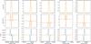Fig. 6 Synthetic intensity in temperature units (upper row), Stokes Q/I (middle row) and V/I (lower row) for five of the most SO representative lines in a cloud model. Blue curves display the results for a field pointing to the observer, while orange shows fields pointing perpendicular to the observer.

The previous considerations are only approximate. For this reason, we have used the results of this paper to synthesize the four Stokes parameter spectra that emerge from a cold cloud assuming a radial magnetic field. To this end, we integrate the radiative transfer equation for polarized radiation along rays at two different impact parameters. This equation is solved using the DELOPAR formal solver, which has second-order precision (Trujillo Bueno 2003). The propagation matrix that we use is the one associated with the Zeeman effect in the linear regime (Landi Degl’Innocenti & Landolfi 2004). Figure 6 shows the observed Stokes parameters (rows) for five of the most interesting SO lines (columns). The intensity is displayed in temperature units, while Stokes parameter Q and V spectra are shown relative to Stokes I.

For simplicity, we assume local thermodynamic equilibrium throughout the whole cloud. This approximation is surely not valid for the Stokes I profile, but its effect on the relative Stokes parameters is minimal. The model that we use is a static isothermal cloud of 15′′ radius at 300 pc, with T = 10 K, n(H₂) = 10⁵ cm^-3, a relative abundance X(SO) = 5 × 10^-9, and B = 1 mG. We assume observations at the cloud center. Concerning the topology of the field, we consider one case with the field pointing to the observer (blue curves) and another one with the field perpendicular to the observer and oriented along the reference positive Stokes Q direction in the plane of the sky (orange curve). Given that, the magnetic field produces a Zeeman splitting much lower than the width of the line, the Stokes V amplitude scales linearly with B_∥, while Stokes Q and U scale as ${\mathit{B}}_{\mathrm{\perp }}^{\mathrm{2}}$.

Even though the transition at 86 GHz presents a large Zeeman splitting, its specific Zeeman pattern produces a very weak Stokes V signal when the field points to the observer because it has . The reversal close to the rest frequency of the line is produced by magneto-optical effects. Much better candidates for detecting the Zeeman effect in SO are the lines at 159, 286, 309 and 329 GHz, with amplitudes of the order of 1% in relative polarization. The sign of Stokes V of the lines at 159 and 329 GHz is opposite to that of the lines at 286 and 309 GHz. This fact can be exploited to check for detections in noisy observations.

Concerning linear polarization, and as usual for weak fields, it is much smaller than Stokes V (three orders of magnitude in our case). The linear polarization produced by the line at 286 GHz is the strongest, reaching 0.008%, almost an order of magnitude larger than the rest. We also point out that the sign of for the lines at 86 and 309 GHz are opposite to those of the other lines considered.

The overall conclusion is that the lines at 159 and 286 GHz are good candidates for detecting the Zeeman effect in SO. The former produces slightly smaller polarization signals, but the line intensity is stronger. The latter produces larger relative polarizations (especially for linear polarization), but the line is weaker.

6. Concluding remarks

Magnetic fields play a fundamental role in star formation processes and the best method to evaluate their intensity is by means of Zeeman effect measurements of atomic or molecular lines. Furthermore, since the derivation of the magnetic field intensity in a given cloud from different species might help in scrutinizing the role of the magnetic field in the cloud dynamical evolution, this work provides an effective experimental-computational strategy for deriving accurate g factors as well as for identifying, for a given molecule, the rotational transitions that show the strongest Zeeman effect. In particular, in the present study, accurate and reliable values for g_s, g_l, and g_r have been obtained for SO.

The Zeeman effect for molecular species thermally emitting in star forming regions have been observed only for OH and CN. While OH lines can be used to probe diffuse gas, CN is more suitable for denser environments. In this context, SO can be classified a very good tool to sample the high-density portion of the gas around the protostar. An instructive example is provided by the recent ALMA observations of SO emission of the protostars L1527, in Taurus, and HH212, in Orion. The abundance (with respect to H₂) of sulfur monoxide is dramatically enhanced to values up to 10^-7 in small (≤50−100 AU) and dense (≥10⁵⁻⁶ cm^-3) regions, thus revealing the accretion shock at the envelope-disk interface (e.g., Sakai et al. 2014a,b; Podio et al. 2015). It is interesting to note that the rotational transitions showing the largest Zeeman shifts are associated with frequencies from 86 GHz to 329 GHz (with the best candidates being the 159 and 286 GHz lines), which lie in the spectral bands of the main interferometers routinely used to investigate the inner portion of star forming regions.

Acknowledgments

This work has been supported in Bologna by MIUR “PRIN 2012, 2015” funds (project “STAR: Spectroscopic and computational Techniques for Astrophysical and atmospheric Research” – Grant Number 20129ZFHFE, project “STARS in the CAOS (Simulation Tools for Astrochemical Reactivity and Spectroscopy in the Cyberinfrastructure for Astrochemical Organic Species)” – Grant Number 2015F59J3R) and by the University of Bologna (RFO funds), in Mainz by the Deutsche Forschungsgemeinschaft (DFG 370/6-1 and 370/6-2). S.C. acknowledges support from the AIAS-COFUND program, grant agreement No. 609033. A.A.R. acknowledges financial support by the Spanish Ministry of Economy and Competitiveness through project AYA2014-60476-P and the Ramón y Cajal fellowships. J.C. thanks spanish MINECO for funding under grants AYA2012-32032, AYA2016-75066-C2-1-P, CSD2009-00038 (ASTROMOL) under the Consolider-Ingenio Program, and the European Research Council under the European Union’s Seventh Framework Programme (FP/2007-2013)/ERC-SyG-2013 Grant Agreement No. 610256 NANOCOSMOS. The support of the COST CMTS-Actions CM1405 (MOLIM: MOLecules In Motion) and CM1401 (Our Astro-Chemical History) is acknowledged.

References

All Tables

All Figures

	Fig. 1 N,J = 4, 3 ← 3, 2 transition of SO at 159.0 GHz: Zeeman spectrum obtained by applying a magnetic field of 22.3 G.
In the text

	Fig. 2 N,J = 2, 2 ← 1, 2 transition of SO at 309.5 GHz: Zeeman spectrum obtained by applying a magnetic field of 11.2 G.
In the text

	Fig. 3 N,J = 9, 8 ← 8, 7 transition of SO at 384.5 GHz: Zeeman spectrum obtained by applying a magnetic field of 111.4 G (in blue); the calculated stick spectrum (in red) is also depicted. In the inset, an example of a single recording is shown.
In the text

	Fig. 4 N,J = 9, 10 ← 8, 9 transition of SO at 389.1 GHz: experimental (in blue) and calculated (in red) Zeeman spectrum obtained by applying a magnetic field of 67 G.
In the text

	Fig. 5 N,J = 3, 2 ← 1, 2 transition of O2 at 424.8 GHz: Zeeman spectrum obtained by applying a magnetic field of 5.7 G.
In the text

	Fig. 6 Synthetic intensity in temperature units (upper row), Stokes Q/I (middle row) and V/I (lower row) for five of the most SO representative lines in a cloud model. Blue curves display the results for a field pointing to the observer, while orange shows fields pointing perpendicular to the observer.
In the text

References

- Aidas, K., Angeli, C., Bak, K. L., et al. 2014, WIREs Comput. Mol. Sci., 4, 269 [CrossRef] [Google Scholar]
- Bai, X.-N., & Stone, J. M. 2013, ApJ, 769, 76 [NASA ADS] [CrossRef] [Google Scholar]
- Bel, N., & Leroy, B. 1989, A&A, 224, 206 [NASA ADS] [Google Scholar]
- Bel, N., & Leroy, B. 1998, A&A, 335, 1025 [Google Scholar]
- Carrington, A., Levy, D. H., & Miller, T. A. 1967, Proc. R. Soc. Lond. Series A, 298, 340 [NASA ADS] [CrossRef] [Google Scholar]
- Cazzoli, G., & Puzzarini, C. 2006, J. Mol. Spectr., 240, 153 [NASA ADS] [CrossRef] [Google Scholar]
- Cazzoli, G., & Puzzarini, C. 2013, J. Phys. Chem. A, 114, 13759 [CrossRef] [Google Scholar]
- Cazzoli, G., Puzzarini, C., & Lapinov, A. V. 2004, ApJ, 611, 615 [NASA ADS] [CrossRef] [Google Scholar]
- Christensen, H., & Veseth, L. 1978, J. Mol. Spectr., 72, 438 [NASA ADS] [CrossRef] [Google Scholar]
- Crutcher, R. M. 2007, in EAS Pub. Ser. 23, eds. M.-A. Miville-Deschênes, & F. Boulanger, 37 [Google Scholar]
- Crutcher, R. M. 2012, ARA&A, 50, 29 [NASA ADS] [CrossRef] [Google Scholar]
- Crutcher, R. M., & Kazés, I. 1983, A&A, 125, L23 [NASA ADS] [Google Scholar]
- Crutcher, R. M., Troland, T. H., Goodman, A. A., et al. 1993, ApJ, 407, 175 [NASA ADS] [CrossRef] [Google Scholar]
- Crutcher, R. M., Troland, T. H., Lazareff, B., & Kazes, I. 1996, ApJ, 456, 217 [NASA ADS] [CrossRef] [Google Scholar]
- Crutcher, R. M., Troland, T. H., Lazareff, B., Paubert, G., & Kazés, I. 1999, ApJ, 514, 121 [Google Scholar]
- Daniels, J. M., & Dorain, P. B. 1966, J. Chem. Phys., 45, 26 [NASA ADS] [CrossRef] [Google Scholar]
- di Francesco, J., Evans, II, N. J., Caselli, P., et al. 2007, Protostars and Planets V, 17 [Google Scholar]
- Engström, M., Minaev, B., Vahtras, O., & Ågren, H. 1998, Chem. Phys., 237, 149 [NASA ADS] [CrossRef] [Google Scholar]
- Epifanovsky, E., Klein, K., Stopkowicz, S., Gauss, J., & Krylov, A. I. 2015, J. Chem. Phys., 143, 064102 [NASA ADS] [CrossRef] [Google Scholar]
- Evenson, K. M., & Mizushima, M. 1972, Phys. Rev. A, 6, 2197 [NASA ADS] [CrossRef] [Google Scholar]
- Frank, A., Ray, T. P., Cabrit, S., et al. 2014, Protostars and Planets VI, 451 [Google Scholar]
- Gauss, J., Ruud, K., & Helgaker, T. 1996, J. Chem. Phys., 105, 2804 [NASA ADS] [CrossRef] [Google Scholar]
- Gauss, J., Ruud, K., & Kállay, M. 2007, J. Chem. Phys., 127, 074101 [NASA ADS] [CrossRef] [PubMed] [Google Scholar]
- Gauss, J., Kállay, M., & Neese, F. 2009, J. Phys. Chem. A, 113, 11541 [CrossRef] [Google Scholar]
- Harriman, J. 1987, Physical Chemistry: A Series of Monographs, Theoretical Foundations of Electron Spin Resonance (New York: Academic Press), 37 [Google Scholar]
- Heckert, M., Kállay, M., & Gauss, J. 2005, J. Chem. Phys., 103, 2109 [Google Scholar]
- Heckert, M., Kállay, M., Tew, D. P., Klopper, W., & Gauss, J. 2006, J. Chem. Phys., 125, 044108 [NASA ADS] [CrossRef] [Google Scholar]
- Helgaker, T., Jørgensen, P., & Olsen, J. 2000, Molecular Electronic-Structure Theory (Chichester: John Wiley & Sons) [Google Scholar]
- Hennebelle, P., & Fromang, S. 2008, A&A, 477, 9 [NASA ADS] [CrossRef] [EDP Sciences] [Google Scholar]
- Hess, B. A., Marian, C. M., Wahlgren, U., & Gropen, O. 1996, Chem. Phys. Lett., 251, 365 [NASA ADS] [CrossRef] [Google Scholar]
- Kaupp, M., Bühl, M., & Malkin, V. G., eds. 2004, Calculation of NMR and EPR Parameters: Theory and Applications (Wiley) [Google Scholar]
- Kawaguchi, K., Yamada, C., & Hirota, E. 1979, J. Chem. Phys., 71, 3338 [NASA ADS] [CrossRef] [Google Scholar]
- Königl, A., & Ruden, S. 1993, Origin of Outflows and Winds, eds. M. Matthews, & E. Levy, Protostars and Planets III (Tucson: Univ. Arizona Press), 641 [Google Scholar]
- Koseki, S., Gordon, M. S., Schmidt, M. W., & Matsunaga, N. 1995, J. Phys. Chem., 99, 12764 [CrossRef] [Google Scholar]
- Koseki, S., Schmidt, M. W., & Gordon, M. S. 1998, J. Phys. Chem. A, 102, 10430 [CrossRef] [Google Scholar]
- Landi Degl’Innocenti, E., & Landolfi, M. 2004, Polarization in Spectral Lines (Kluwer Academic Publishers) [Google Scholar]
- Landman, D. A., Roussel-Dupré, R., & Tanigawa, G. 1982, ApJ, 261, 732 [NASA ADS] [CrossRef] [Google Scholar]
- Lattanzi, V., Cazzoli, G., & Puzzarini, C. 2015, ApJ, 813, 4 [NASA ADS] [CrossRef] [Google Scholar]
- Li, H.-B., Goodman, A., Sridharan, T. K., et al. 2014, Protostars and Planets VI, 101 [Google Scholar]
- Martin, E. V. 1932, Phys. Rev., 41, 167 [NASA ADS] [CrossRef] [Google Scholar]
- Martin-Drumel, M. A., Hindle, F., Mouret, G., Cuisset, A., & Cernicharo, J. 2015, ApJ, 799, 115 [NASA ADS] [CrossRef] [Google Scholar]
- Mills, I., Cvitaš, T., Homann, K., Kallay, N., & Kuchitsu, K. 1993, Quantities, Units and Symbols in Physical Chemistry, 2nd edn. (London: Blackwell Science) [Google Scholar]
- Momjian, E., & Sarma, A. P. 2017, ApJ, 834, 168 [NASA ADS] [CrossRef] [Google Scholar]
- Neese, F. 2001, J. Chem. Phys., 115, 11080 [NASA ADS] [CrossRef] [Google Scholar]
- Neese, F. 2005, J. Chem. Phys., 122, 034107 [NASA ADS] [CrossRef] [Google Scholar]
- Pillai, T., Kauffmann, J., Wiesemeyer, H., & Menten, K. M. 2016, A&A, 591, A19 [NASA ADS] [CrossRef] [EDP Sciences] [Google Scholar]
- Podio, L., Codella, C., Gueth, F., et al. 2015, A&A, 581, A85 [NASA ADS] [CrossRef] [EDP Sciences] [Google Scholar]
- Purvis III, G. D., & Bartlett, R. J. 1982, J. Chem. Phys., 76, 1910 [NASA ADS] [CrossRef] [Google Scholar]
- Puzzarini, C., Cazzoli, G., & Gauss, J. 2012, J. Chem. Phys., 137, 154311 [NASA ADS] [CrossRef] [Google Scholar]
- Raghavachari, K., Trucks, G. W., Pople, J. A., & Head-Gordon, M. 1989, Chem. Phys. Lett., 157, 479 [NASA ADS] [CrossRef] [Google Scholar]
- Roos, B. O., Taylor, P. R., & Siegbahn, P. E. M. 1980, Chem. Phys., 48, 157 [NASA ADS] [CrossRef] [MathSciNet] [Google Scholar]
- Sakai, N., Oya, Y., Sakai, T., et al. 2014a, ApJ, 791, L38 [NASA ADS] [CrossRef] [Google Scholar]
- Sakai, N., Sakai, T., Hirota, T., et al. 2014b, Nature, 507, 78 [NASA ADS] [CrossRef] [Google Scholar]
- Shavitt, I., & Bartlett, R. J. 2009, Many-Body Methods in Chemistry and Physics: MBPT and Coupled-Cluster Theory (Cambridge: Cambridge University Press) [Google Scholar]
- Shinnaga, H., & Yamamoto, S. 2000, ApJ, 544, 330 [NASA ADS] [CrossRef] [Google Scholar]
- Stanton, J. F., Gauss, J., Harding, M. E., et al. 2016, CFOUR A quantum chemical program package, for the current version, see http://www.cfour.de [Google Scholar]
- Trujillo Bueno, J. 2003, in Stellar Atmosphere Modeling, eds. I. Hubeny, D. Mihalas, & K. Werner (San Francisco: ASP), ASP Conf. Ser., 288, 551 [Google Scholar]
- Uchida, K. I., Fiebig, D., & Güsten, R. 2001, A&A, 371, 274 [NASA ADS] [CrossRef] [EDP Sciences] [Google Scholar]
- Vahtras, O., Minaev, B., & Ågren, H. 1997, Chem. Phys. Lett., 281, 186 [NASA ADS] [CrossRef] [Google Scholar]
- Vahtras, O., Engström, M., & Schimmelpfennig, B. 2002, Chem. Phys. Lett., 351, 424 [NASA ADS] [CrossRef] [Google Scholar]
- van Dishoeck, E. F., & Blake, G. A. 1998, ARA&A, 36, 317 [NASA ADS] [CrossRef] [Google Scholar]
- Vázquez, J., Harding, M. E., Stanton, J. F., & Gauss, J. 2011, J. Chem. Theor. Comp., 7, 1428 [CrossRef] [Google Scholar]
- Vlemmings, W. H. T. 2007, in Astrophysical Masers and their Environments, eds. J. M. Chapman, & W. A. Baan, IAU Symp., 242, 37 [Google Scholar]
- Winnewisser, M., Sastry, K. V. L. N., Cook, R. L., & Gordy, W. 1964, J. Chem. Phys., 41, 1687 [NASA ADS] [CrossRef] [Google Scholar]
- Woon, D., & Dunning, T. 1993, J. Chem. Phys., 98, 1358 [CrossRef] [Google Scholar]
- Woon, D., & Dunning, T. 1995, J. Chem. Phys., 103, 4572 [NASA ADS] [CrossRef] [Google Scholar]
- Yu, S., Miller, C. E., Drouin, B. J., & Müller, H. S. P. 2012, J. Chem. Phys., 137, 024304 [NASA ADS] [CrossRef] [PubMed] [Google Scholar]
All Tables
Rotational transitions of SO for the preliminary investigation of the Zeeman effect.