| Issue |
A&A
Volume 605, September 2017
|
|
|---|---|---|
| Article Number | A60 | |
| Number of page(s) | 10 | |
| Section | Astrophysical processes | |
| DOI | https://doi.org/10.1051/0004-6361/201730523 | |
| Published online | 11 September 2017 | |
What can we learn from “internal plateaus”? The peculiar afterglow of GRB 070110
1 UPMC-CNRS, UMR 7095, Institut d’Astrophysique de Paris, 75014 Paris, France
e-mail: This email address is being protected from spambots. You need JavaScript enabled to view it.
2 Department of Physics, The George Washington University, Washington, DC 20052, USA
Received: 30 January 2017
Accepted: 6 May 2017
Abstract
Context. The origin of the prompt emission of gamma-ray bursts is highly debated. Proposed scenarios involve various dissipation processes (shocks, magnetic reconnection, and inelastic collisions) above or below the photosphere of an ultra-relativistic outflow.
Aims. We search for observational features that could help to favour one scenario over the others by constraining the dissipation radius, the magnetization of the outflow, or by indicating the presence of shocks. Bursts showing peculiar behaviours can emphasize the role of a specific physical ingredient, which becomes more apparent under certain circumstances.
Methods. We study GRB 070110, which exhibited several remarkable features during its early afterglow; i.e. a very flat plateau terminated by an extremely steep drop and immediately followed by a bump. We modelled the plateau as the photospheric emission from a long-lasting outflow of moderate Lorentz factor (Γ ~ 20), which lags behind an ultra-relativistic (Γ > 100) ejecta that is responsible for the prompt emission. We computed the dissipation of energy in the forward and reverse shocks resulting from the deceleration of this ejecta by the external medium (uniform or stellar wind).
Results. We find that photospheric emission from the long-lasting outflow can account for the plateau properties (luminosity and spectrum) assuming that some dissipation takes place in the flow. The geometrical timescale at the photospheric radius is so short that the observed decline at the end of the plateau likely corresponds to the actual shutdown of the activity in the central engine. The bump that follows results from the power dissipated in the reverse shock, which develops when the material making the plateau catches up with the initially fast shell in front, after the fast shell has decelerated.
Conclusions. The proposed interpretation suggests that the prompt phase results from dissipation above the photosphere while the plateau has a photospheric origin. If the bump is produced by the reverse shock, it implies an upper limit (σ ≲ 0.1) on the magnetization of the low Γ material making the plateau. A plateau that is terminated by a drop as steep as in GRB 070110 was not observed in any other long burst. It could mean that persistent outflows are very uncommon or that the plateau luminosity or the energy of the emitted photons are generally much lower because the outflow remains mostly adiabatic or has a Lorentz factor below 10.
Key words: gamma-ray burst: general / gamma-ray burst: individual: 070110 / radiation mechanisms: non-thermal / radiation mechanisms: thermal / relativistic processes
© ESO, 2017
1. Introduction
The Swift and Fermi satellites, launched in 2004 and 2008, respectively, have dramatically improved our knowledge of the observational properties of gamma-ray bursts (GRBs). The rapid slewing capabilities of Swift and its narrow field X-ray and visible instruments XRT and UVOT have revealed the rich phenomenology of the early afterglow and have allowed a redshift determination for nearly 500 bursts. The broad spectral coverage with Fermi GBM and LAT from a few keV to the GeV range has shown in some cases the presence of additional components to the simple Band spectrum such as power-law spectra extending to very high energies (Swenson et al. 2010; Guetta et al. 2011; Beniamini et al. 2011; Ackermann et al. 2013) or possible thermal emission from the photosphere (Guiriec et al. 2011; Axelsson et al. 2012).
On the theoretical side, the dissipation process responsible for the prompt emission remains uncertain. There are three main contenders: internal shocks (Rees & Meszaros 1994; Kobayashi et al. 1997; Daigne & Mochkovitch 1998, 2000; Beloborodov 2000; Bošnjak et al. 2009), magnetic reconnection (Usov 1994; Drenkhahn & Spruit 2002; Giannios 2008; Zhang & Yan 2011; McKinney & Uzdensky 2012; Sironi et al. 2015; Beniamini & Granot 2016; Granot 2016; Kagan et al. 2016; Beniamini & Giannios 2017), or dissipative photosphere (Thompson 1994; Ghisellini & Celotti 1999; Mészáros & Rees 2000; Rees & Mészáros 2005; Pe’er et al. 2005; Giannios & Spruit 2007; Lazzati & Begelman 2010; Beloborodov 2010; Levinson 2012; Beloborodov 2013), which differ in terms of emission radii and radiative mechanisms. Internal shocks and magnetic reconnection dissipate kinetic and magnetic energy in the flow, respectively; the flow is then radiated above the photosphere, typically via the synchrotron process (Katz 1994; Rees & Meszaros 1994; Sari et al. 1996; Kumar & McMahon 2008; Daigne et al. 2011; Beniamini & Piran 2013, 2014). In photospheric models dissipation below the photosphere produces energetic electrons that can transform a seed Planck spectrum into a broken power law with inverse Compton (IC) collisions contributing to the high-energy emission and an additional synchrotron component at low energies (Thompson 1994; Mészáros & Rees 2000; Giannios 2006; Beloborodov 2010; Lazzati & Begelman 2010; Vurm et al. 2011; Giannios 2012).
Various proposals have been made to explain the unexpected features of the early afterglow (extended plateaus, flares, steep breaks) often involving long-term activity of the burst central engine or alternatively the contribution of a long-lived reverse shock (Uhm & Beloborodov 2007; Genet et al. 2007). This observational diversity can be seen as a source of confusion and it certainly is in some respects. However, peculiarities could also result from one or several ingredients of the model taking non-standard values. In this case, these bursts can in fact provide clues to elucidate the physics at work. We concentrate here on GRB 070110 and use it as a laboratory to constrain the dissipation process, the importance of photospheric emission, and the role played by the reverse shock.
GRB 070110 started with a rather regular prompt emission (see Sect. 2). Swift XRT observations followed at 100 s and showed the usual early steep decay with the X-ray flux FX(t) ∝ t-2.53. After a data interruption due to orbit constraints, the XRT light curve exhibited a very flat plateau from a few 103 s to 18 000 s (300–5400 s in the burst rest frame at z = 2.35). This plateau ended with a very steep drop (FX(t) ∝ t-9). Remarkably, the plateau is not seen in simultaneous observations with the UVOT instrument, which shows a regular power-law behaviour.
The initial decay following the prompt phase can be explained as high-latitude emission from the final emitting shell at R ~ 2 cΓ2τ, where τ is the duration of the prompt activity. This value for the radius is naturally expected in internal shocks models (e.g. Kobayashi et al. 1997; Hascoët et al. 2012) and in some reconnection models (e.g. Beniamini & Granot 2016). Conversely, in photospheric models, where the emission radius is much smaller, this geometrical interpretation does not work and the decay should correspond to an effective decline of the activity in the central engine. In some respects, the situation at the end of the plateau is just the opposite: the drop is much too steep to be related to either a forward or reverse shock contribution. This has led to the idea of “internal plateaus” (Zhang et al. 2006; Liang et al. 2006; Troja et al. 2007), where the dissipation radius is much closer to the central source. The geometrical timescale R/ 2cΓ2 can then be very short but the physical timescale for the decay of source activity must also be short, since the observed decline is controlled by the longest of the two.
One possible way to obtain a short physical decay timescale is to suppose that the central source that powers the plateau is a magnetar that eventually collapses to a black hole. However, a short decay timescale also requires a short geometrical timescale. The latter could be naturally produced if the plateau results from photospheric emission. We discuss these two possibilities below. After a short summary of the observational properties of GRB 070110 in Sect. 2, we consider the magnetar hypothesis in Sect. 3. Section 4 compares the photospheric emission of a steady outflow to the plateau data while Sect. 5 presents the forward and reverse shock contributions to the afterglow. Our results are discussed in Sect. 6, which is also the conclusion.
2. GRB 070110: brief summary of the observational properties
The prompt phase of GRB 070110 was not especially remarkable. It lasted 90 s (t90 [15–150 keV] = 89 ± 7 s) with an initial peak followed by 4–5 overlapping pulses during the first 40 s and a tail for the next 50 s. The time-averaged photon spectrum could be fitted by a single power law of index 1.57, which did not allow the peak energy to be constrained. The isotropic energy released in the BAT spectral range 15–150 keV (50–500 keV in burst rest frame) was Eiso,BAT = 2.3 × 1052 erg. Assuming that the spectrum keeps the same slope from 0 to the peak energy Ep ≥ 500 keV and then breaks to a photon index β> 2, the total isotropic energy would be  (1)The flux at the end of the prompt phase decays as t-2.45, which is typical of the evolution observed in most GRBs. The plateau phase that follows is very flat and extends to 20 ks (or τplateau = 5800 s in the rest frame) with a luminosity Lplateau ~ 1048 erg s-1 within the XRT spectral range, which covers 1.5 decades in energy. This value of the luminosity therefore corresponds to a lower limit. If the spectrum keeps the same slope (F(E) ~ E-1) in an interval [E1,E2] covering d > 1.5 decades the corrected luminosity is Lplateau ~ 1048 (d/ 1.5) erg s-1, leading to a total energy radiated during the plateau phase Eplateau = Lplateau × τplateau = 5.8 1051 (d/ 1.5) erg.
Since the plateau is not seen at optical wavelengths the observed spectrum should break at some energy below the lower bound of the XRT range of 0.3 keV. This implies an average slope s < 0.4 (with F(E) ∝ E− s) in the interval from 0.3 keV to the optical. The plateau abruptly ends with the X-ray flux decreasing as t-9, or on a (observed) timescale of about 5000 s, corresponding to δτplateau/τplateau ~ 0.25. This implies that the plateau emission cannot come from either the forward or reverse shocks, which would imply δτplateau/τplateau ~ 1.
Just following the drop, a bump is observed in the XRT light curve with an increase of the flux by a factor of 3 and a total duration of about 105 s (Troja et al. 2007). We lack optical wavelength data so it is not possible to know if the bump would have also been visible in the optical light curve. A possible second weaker bump is also seen immediately after the first bump before the X-ray light curve recovers a power-law decline of temporal index α ≈ −0.6. As noted by Troja et al. (2007), this decay does not follow the regular closure relations as expected in the forward afterglow scenario, given the spectral index measured in the X-ray band at the same time (approximately Fν ∝ ν-1.1).
The most striking feature in the afterglow of GRB 070110 is clearly the very steep drop at the end of the plateau, which contrasts with the standard decay at the end of the prompt phase. This internal plateau must be directly related to the activity of the central engine, showing that at least in some bursts it can still operate (at a reduced level) for a duration that can exceed that of the prompt phase by more than two orders of magnitude.
3. Origin of the plateau: magnetar hypothesis
Several studies have suggested a spinning down highly magnetized pulsar, known as a magnetar, as the origin for the plateau of GRB 070110 (Troja et al. 2007; Lyons et al. 2010; Yu et al. 2010; Du et al. 2016). The magnetar solution must satisfy two main constraints: (i) the available energy reservoir should be able to power the plateau for 1.5 h and (ii) the subsequent drop of luminosity should be steep enough. For a dipole spin-down mechanism, the released power at t>ts, where ts is the starting time of the spin-down, can be written as  (2)where
  is the observed spin-down time of the pulsar and depends on the dipolar magnetic field strength at the poles (Bp), the pulsar’s moment of inertia (I), radius (R), and initial spin frequency (Ω0). The initial power is then given by the ratio of the initial rotational energy to the spin-down time, i.e.
  . One therefore expects a constant power L0 up to t0 followed by a power-law decline. If this power is directly translated to the observed X-ray plateau, it is possible to link the observed luminosity and duration to the initial magnetar parameters, i.e. Bp and Ω0. Indeed, applying this method to GRB 070110, assuming I = 1045 gcm2,R = 106 cm, Troja et al. (2007) find Bp ≳ 3 × 10¹⁴ Gauss and P0 ≡ 2π/ Ω0 ≲ 1 ms. The magnetar should therefore be spinning very close to the break-up limit (Lattimer & Prakash 2004) with P0 = 0.96 ms. This implies that unless almost all of the spin-down luminosity is translated to the observed X-ray emission, the energetic requirements may be too large to be accounted for by a magnetar.
However, this calculation has two important caveats. First, it assumes 100% efficiency in translating the luminosity of the magnetar to the observed luminosity in X-rays. Furthermore, it implicitly assumes that the flux is rather sharply peaked in the X-ray band, possibly suggesting a thermal spectrum and photospheric origin for this emission (see further discussion of the spectrum in Sect. 4.2). Secondly, it assumes that the luminosity is released isotropically. Breaking the first of these assumptions would require even more energy at the source while the second assumption reduces the energy requirements. A full assessment of the magnetar parameters in this model (and its viability from an energetic point of view) therefore crucially depends on the efficiency of energy conversion and on the opening angle of the jet. Regardless of the implied magnetar parameters, a preliminary question that has to be addressed in this scenario is: what accounts for the prompt emission? If the magnetar spin-down luminosity is associated with that of the plateau then it seems unlikely that it could also be associated with the prompt emission, which involves different luminosities and timescales (see Sect. 2; see also Granot et al. 2015).
As pointed out by Troja et al. (2007), the rapid decay at the end of the plateau (at tobs ~ 2 × 10⁴ s) suggests an “internal” origin for the plateau emission, i.e. the power of the magnetar should be dissipated at a radius well below that of the forward shock, indicating that the emission cannot be simply due to energy injection (e.g. Zhang & Mészáros 2001). This is because the observed decay is on a timescale tdecay < 5 × 10³ s, which is significantly shorter than the angular timescale associated with the forward shock material at that time, tθ = R(1 + z)/2cΓ2 ~ tobs ~ 2 × 10⁴ s. Also, the energy of the magnetar cannot be emitted directly from its surface as the magnetar is highly super-Eddington. This leads to a lower limit on the radius and Lorentz factor at the dissipation radius. Therefore, in the context of the magnetar model, one must still find some alternative way of dissipating the power as well as explaining why the emission should reside predominantly in X-rays.
An additional concern for the magnetar model has to do with the shape of the decline at the end of the plateau. Namely, the decline expected from a dipole spin-down (Eq. (2)) is too shallow as compared with observations. For a general spin-down mechanism, one can write  (3)where the expression in Eq. (2)is restored for n = 3. In Fig. 1 we plot this function for a range of values of n = 1−3 (n = 1–2.8 is the typically inferred range from observations of isolated pulsars; e.g. Hamil et al. 2015); we compare these results with the observed light curve. Generally, the slope becomes steeper as n decreases, but even for n = 1, it is clear that the drop is too shallow as compared with observations. An alternate possibility, is that the spin-down stops abruptly due to the collapse of the rotating neutron star to a black hole. This could produce an almost step-like drop in the light curve, but may require fine-tuning in order for the collapse to happen at tcoll ≈ t0 or else, if tcoll ≪ t0, would require even higher values for the initial energy of the magnetar, which is already uncomfortably close to the maximum theoretical value.
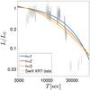 |
Fig. 1 Normalized luminosity (L/L0) as a function of time (see Eq. (3)) for various spin-down models (n = 1,2,3) as compared with the observed XRT data. We take t0 = 2 × 10⁴ s, which is the observed time of the end of the plateau, and ts = 4000 s, which is the observed time at which the plateau starts and is an upper limit on the actual value. |
4. Photospheric emission from a relativistic outflow
4.1. Basic equations: non-dissipative outflow from the central engine to the photosphere
Considering the various potential issues with the magnetar hypothesis outlined above, we suggest a simple alternative where the central engine is instead powered by a black hole. In this scenario the central engine transitions from an initial phase with high injected power driving a jet of large Lorentz factor (several hundreds) responsible for the prompt emission to a second phase with much lower injected power driving a slower outflow with a Lorentz factor of a few tens only1. The plateau corresponds to the photospheric emission from this slower outflow. We suppose first that the outflow is non-dissipative and starts with Γ0 ≈ 1 from an initial radius R0, close to the central engine (i.e. R0 ≲ 107 cm). This outflow then accelerates and expands adiabatically up to the photosphere. The initial temperature T0 at the origin can be estimated by  (4)where Ė is the total power injected in the flow, ϵth is the fraction of that energy in thermal form, and a is the radiation constant. This leads to
  (5)where here and elsewhere in the text we use the notation qx for q in units of 10x in cgs. Since at the base of the jet, the temperature is already below the pair creation threshold (and at larger radii the temperature only further decreases), we can safely ignore the effects of pair creation within the flow. In addition, in order for the photospheric emission from this material to be able to account for the X-ray plateau, we can also assume that the flow has stopped accelerating by the time it reaches the photosphere. This is because, otherwise, assuming a pure fireball in which the acceleration persists as Γ ∝ r, the observed peak of the photospheric component would have been ≈kBT0/ (1 + z) ≈ 300 keV (e.g. Kumar & Zhang 2015), and the contribution of this emission at the observed [0.1,10] keV X-ray band would have been too small2. With these assumptions, the luminosity at the photosphere takes the form
 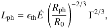 (6)where Rph is the photophereric radius and Γ is the Lorentz factor at Rph. Similarly, the observed temperature is given by
  (7)The photospheric radius can be expressed by (see also Zhang & Yan 2011)
  (8)where σT is the Thomson cross section, mp the proton mass, and σ the magnetization of the flow such that ĖK = Ė/ (1 + σ) is the injected kinetic power. Using Eqs. (6)–(8) we obtain
  (9)and
  (10)It is illustrative to consider the ratio Lph/Tobs, since it is independent of Γ and relatively insensitive to the other model parameters, yet can still be compared directly to observations. We find
  (11)Applying this expression to GRB 070110 during the plateau phase with Lph = 1048 erg s-1, Tobs ≈ 1 keV and R0 = 107 cm we obtain ϵthĖ50 ≈ 1. With a plateau duration of about 5800 s (rest frame), the total (isotropic equivalent) energy released by the central engine during this phase should be E = 6 × 1053/ϵth erg, which, for ϵth smaller than unity, becomes uncomfortably large. We assume here that the emitted power during the plateau falls predominantly in the [0.1–10] keV range observed by Swift XRT. If this is not the case the energetic requirements become even larger. The possibility of powering the observed plateau from a non-dissipative photosphere is therefore disfavoured. In what follows we thus turn to a discussion of dissipative photospheres.
4.2. Flow propagation with dissipation
A larger efficiency can be achieved if dissipation takes place in the outflow between the initial injection radius R0 and the photosphere, Rph. Furthermore, if the jet undergoes strong dissipation below the photosphere, it could result in a strong photospheric signal, even if the flow is initially strongly magnetically dominated. Hence, the required photospheric component in our model does not necessarily impose a baryonic jet. The general tendency is that the lower the dissipation occurs below the photosphere (i.e. the higher the optical depth at the dissipation radius) and the lower the initial energy per Baryon, the more thermal-like would be the resulting signal. This has been studied in many works, such as Pe’er & Waxman (2004), Giannios & Spruit (2005), Giannios (2006), Giannios & Spruit (2007), Beloborodov (2011) and Vurm et al. (2011). If dissipation happens mostly at a large optical depth, it can increase the efficiency but the resulting spectrum remains close to a blackbody. However, if dissipation extends all the way to the photosphere, Comptonization of the thermal photons by energetic electrons can replace the exponential cut-off of the Planck function by an extended power law.
In the first case the expected spectrum is a combination of a blackbody component from the plateau with a power-law component from the underlying afterglow. This possibility, is however unlikely, given that attempting to fit the XRT spectrum at the time of the plateau with a blackbody + power law model, we find that in the spectral interval 0.5–2 keV (observer frame), the thermal flux is at most (at the 3 sigma level) 0.28 of the flux of the power law in the same band. This clearly demonstrates that the plateau emission cannot be dominated by a pure blackbody component.
The observed X-ray spectrum at the time of the plateau, after correcting for dust absorption, was fitted with a simple power law Fν ∝ ν-1 (Troja et al. 2007). Since the burst is high redshift (z = 2.35), the dust absorption is dominated by the intergalactic rather than the galactic component. There is therefore relatively small uncertainty in the dust reduction process. However, the ν-1 power law cannot be the end of the story. This is because its extension to the optical band would strongly over-predict the observed flux in that band. In addition, as mentioned in Sects. 3 and 4.1, the energetic requirements for the plateau are already very large. Unless a cut-off or a significant break in the spectrum both below and above the XRT range are invoked, these requirements would quickly become unmanageable. This suggests that even if the plateau emission is not purely thermal, it clearly cannot be a pure power law either and it is useful to consider other possibilities. Indeed we find that a Planck-like function, where the exponential cut-off is replaced by a power law approaching Fν ∝ ν-1 (which can be naturally obtained assuming strong Comptonization effects take place close to the photosphere; see Giannios & Spruit 2007), overcomes the difficulties described above and is consistent with the data, as long as the temperature is ≲0.5 keV.
In the case of a Comptonized photosphere we introduce two dimensionless parameters to account for energy dissipation and deviation from a blackbody spectrum. These are ϵrad and λ, respectively, which are defined by  (12)where σS and k are the Stefan and Boltzmann constants and Ep is the peak energy of the spectrum in the source rest frame. The parameter λ is smaller or equal to unity with equality corresponding to a pure (not Comptonized) Planck spectrum; ϵrad is equal or larger than the efficiency of a non-dissipative photosphere, which using Eq. (9)gives
  (13)From Eq. (12)and the expression of the photospheric radius
  (14)we can obtain the Lorentz factor at the photosphere
  The Lorentz factor of the slower moving material is therefore rather insensitive to the model parameters. As mentioned in Sect. 4.1, if the flow has not reached the saturation radius at the photosphere, the terminal Lorentz factor could be larger (and Eq. (15)would be considered as a minimum on its actual value). However, this possibility is unlikely for Γs ≲ 20 and would in any case lead to a peak that is significantly higher than the observed band. We therefore do not consider this possibility in the following. Plugging Eq. (15)back into Eq. (14)we find
  (17)with a corresponding geometric timescale
  (18)where the observed peak energy, Ep,obs, is in keV (a redshift z = 2.35 was assumed). The actual values of Γ, Rph, and tgeo depend on the uncertain parameters ϵrad, λ, and (1 + σ). Considering, for example, a Comptonized photosphere with λ ~ 0.3 and a magnetization parameter (1 + σ) ~ 2, the Lorentz factor is only reduced by ≈2 compared to the case with λ = (1 + σ) = 1, while the photospheric radius is increased by ≈5 and the geometrical timescale becomes ≈24 times smaller.
It can be seen that, except for very small values of λ or/and Ep,obs, the geometric timescale remains much shorter than the observed decay time at the end of the plateau, which is close to 1.5 h. This indicates that the observed decline effectively corresponds to the physical extinction of the central engine.
5. Revere and forward shock contributions
5.1. Dissipated power and reverse shock re-brightening
The relativistic ejecta emitted by the central engine of GRB 070110 is structured in two shells. The first shell, which has a Lorentz factor of a few hundred is decelerated first and is responsible for the standard afterglow (i.e. excluding the internal plateau) until the second slower shell with a Lorentz factor of a few tens is able to catch up. This second shell may be structured, with an initial outflow lasting 1.5 h (rest frame) with a nearly constant Γ to make the plateau, followed by a tail where Γ decreases to non-relativistic values close to unity. This slow part adds energy to the forward shock and, if its magnetization is low enough, it is crossed by a reverse shock. The crossing time of the region with a constant Lorentz factor is short, leading to a sharp increase in dissipated power, which may explain the bump in the XRT light curve that follows the plateau.
To test this possibility we calculated the dissipated power in the reverse shock following the method described by Genet et al. (2007). We adopted a Lorentz factor Γf = 200 and an injected kinetic power Ėf = 2 × 1052 erg s-1 for a duration of 30 s (rest frame) in the ejecta responsible for the prompt emission. The Lorentz factor can be expected to be highly variable in this initial part of the flow and the value Γf = 200 therefore represents some typical average. This fast part is then followed by a slower long lasting outflow with Γs = 20, Ės = 2 × 1049 erg s-1 and a duration of 5800 s, which makes the plateau. The power dissipated when the reverse shock crosses this material is shown in Fig. 2 for a uniform medium of density n = 30 cm-3 and a stellar wind with A∗ = 2.4. It is proportional to the bolometric luminosity of the reverse shock in case the radiative efficiency is constant and the electrons are in the “fast cooling” regime.
The sharp increase in dissipated power happens when the reverse shock encounters the low Γ tail of the ejecta. The Lorentz factor of the material in the reverse shock is approximated by  (19)where Ms = Es/ Γsc2, Mf = Ef/ Γf(t = 0)c2 are the masses of the slow and fast shells, Mex is the mass of external medium swept up by the shock, Γi ≈ Γf is the Lorentz factor associated with internal motions in the shocked external medium (see Genet et al. 2007, for a detailed description), and tb is the time of the bump, i.e. the time of collision between the slow and fast shells. To estimate this time, we first relate the radius and (source frame) time for the fast moving shell
  (20)where the subscript d denotes quantities at the deceleration radius and ϵ = 3/2 for ISM (ϵ = 1/2 for wind). The slow moving jet is moving in the path evacuated by the fast shell, and thus propagates with a constant Lorentz factor:
  . Requiring that the two shells reach a shared radius at the same time, we plug the latter expression for R in Eq. (20)and obtain an equation for the collision time, t
 (21)At the limit of t ≫ td we obtain
  (22)which can be rewritten as
 for a uniform medium and a stellar wind, respectively, where the index s denotes the slower moving material and f the fast moving material. As shown by Kumar & Piran (2000), this is the time necessary for the fast moving material to decelerate to Γs/ 2 for a uniform medium (Γs/
 for wind). Its value strongly depends on Γs but for the parameters of GRB 070110 required to explain the plateau via photospheric emission (Γs ~ 20, typically; see Sect. 4) we can expect a bump at ~104 s in the burst rest frame (as indeed implied by observations) provided that the density of the external medium is sufficiently large, i.e. n ≈ 30 cm-3 or A∗ ≈ 2.4 for a wind. Owing to the strong dependence of tb on Γ, even a slight change in Γ would have a large effect. For instance, if the terminal Lorentz factor was 25 instead of 20, A∗ and n could be reduced by a factor of 2, to about 1 and 16 cm-3, respectively.
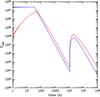 |
Fig. 2 Dissipated power as a function of time for a fast shell of material (Γ ≈ 200) that decelerates into the external medium and is eventually overtaken by a slower outflow, where Γ = 20. Results are shown for a uniform medium of density n = 30 cm-3 (red) and a stellar wind with A∗ = 2.4 (blue). |
5.2. X-ray and visible light curves
In order to calculate the light curves at a given observed frequency, one must specify the microphysical shock parameters ϵe,ϵB as well as the power law slope for the electrons’ energy distribution, p. Since the forward shock is an ultra-relativistic shock, whereas the reverse shock is only mildly relativistic, it is quite likely that these parameters vary from one environment to the other. Many afterglow studies have constrained the values of the microphysical parameters at the forward shock ϵe,f,ϵB,f. The value ϵe,f is strongly constrained by both afterglow modelling (Santana et al. 2014) and numerical simulations of shock acceleration (Sironi & Spitkovsky 2011) to ϵe,f ≈ 0.1. Furthermore, clustering of LAT light curves implies that the distribution around this value is quite narrow (Nava et al. 2014) and finally it cannot be much lower to avoid un-physically large energetic requirements for the blast wave. The value of ϵB,f is less certain. Various recent studies suggest 10-6<ϵB,f< 10-2 (Lemoine et al. 2013; Wang et al. 2013; Barniol Duran 2014; Santana et al. 2014; Zhang et al. 2015; Beniamini et al. 2015, 2016; Burgess et al. 2016). For the reverse shock, there are much less data and the situation is less clear. Following the available estimates in the literature (Fan et al. 2002; Kobayashi & Zhang 2003; McMahon et al. 2006; Shao & Dai 2005), however, we adopt here as canonical values ϵe,r = 0.1 and leave ϵB,r as a free parameter. Reducing either ϵe,r or ϵB,r would decrease the strength of the bump due to the reverse shock as we show explicitly below (Eq. (25)). Finally, we take p = 2.15 for both the reverse and forward shock. This value of p is typical for GRB modelling and is well constrained by comparing the X-ray and optical fluxes during the regular forward afterglow stage (at times later than the plateau and the following bump) and assuming that both are above the cooling break. This assumption is further supported by the fact that the flux in the two bands declines at the same rate as a function of time3. The afterglow of GRB 070110 does not follow the regular closure relations expected in the forward afterglow scenario (see Sect. 2). In other words, the value of p implied by the spectrum does not match the value implied by the temporal behaviour. The most natural way to resolve this apparent contradiction, as indeed pointed out by Troja et al. (2007), is to invoke late-time continuous energy injection. This would both enhance the forward shock emission and lead to a prolonged reverse shock emission, which under certain conditions could dominate the post-plateau light curve. In fact this can be viewed as further evidence for the association of the bump itself with energy injection, and thus of the plateau with emission from this extra material. In order to match the observed post-bump decline, we adopted here a tail component to the slow material, lasting for 400 s (source frame), with Ėt = Ės, and with Γ declining from Γ ≈ 20 down to Γ ≈ 1 with Γ(tinj) ∝ (tf−tinj)2/11, where tinj is the time of injection of a given shell of matter and tf is the time of injection for the final shell.
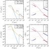 |
Fig. 3 Light-curves corresponding to reverse and forward shock emission assuming the ejecta responsible for the prompt emission is followed by slower moving outflow with Γs = 20, Ės = 2 × 1049 erg s-1 and lasting 6000 s, which makes the plateau. The tail of this material is characterized by the same Ė, lasting 400 s and with a declining Lorentz factor from Γ ≈ 20 down to Γ ≈ 1 with Γ(tinj) ∝ (tf−tinj)2/11. The reverse shock crossing this material accounts for a bump in the afterglow data. The time of the bump and the flux levels during and after the bump match the observed levels. We assume here A∗ = 2.2,ϵe,f = 0.1,ϵB,f = 2.5 × 10⁻⁵,ϵe,r = 0.1,ϵB,r = 4 × 10⁻³,p = 2.15. The top panels correspond to the 1 keV light curve and the bottom panels correspond to the 1 eV light curve. Left: light curve for the reverse shock (blue dot-dashed line) and forward shock (red dashed line). A yellow solid line depicts the sum of the reverse and forward shock contributions. Right: the plots show the evolution of νc,R (blue circles), νm,R (red pluses), νc,f (yellow dashed line) and νm,f (purple dot-dashed line). The observed frequency is depicted by a horizontal line. |
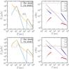 |
Fig. 4 Same as Fig. 3 for an ISM medium with n0 = 30 cm-3. The choice of burst parameters is the same as in Fig. 3 except for ϵB,f = 10-4,ϵB,r = 2 × 10⁻². |
Given these parameters, we calculate the synchrotron flux from the forward shock (Granot & Sari 2002). For the reverse shock we estimate the physical conditions as specified in Genet et al. (2007). In both cases we include possible IC losses including Klein-Nishina corrections (see Sari & Esin 2001; Nakar et al. 2009; Beniamini et al. 2015 for details). Inverse Compton losses become significant for small values of ϵB. Importantly, for these low magnetizations, the X-ray emission from the forward shock is very inefficient because of IC losses of the electrons emitting in the fast cooling synchrotron regime (Sari & Esin 2001). This is in fact essential in our model to allow for a significant contribution from the reverse shock at the time of the bump (and after), without investing an amount of energy in the slow shell that would be considerably larger than the energy stored in the fast component. Indeed, the jet approximately dissipates (all of) its energy on a timescale of order the dynamical time, so if this energy is efficiently radiated as synchrotron in the X-ray regime, the only way to significantly increase the flux would be to significantly increase the energy. Avoiding an energy that is too large in the slow shell is important both on grounds of the total available energy budget and more directly, since such a large energy is not seen during the plateau emission. The low values of ϵB, motivated by values found in the literature, suppress the synchrotron flux from IC losses. Thus, these values can allow for a significant contribution from the reverse shock without investing huge amounts of energy in the latter component, assuming that in the reverse shock, ϵB is not as small as in the forward shock.
Using the values of the parameters described above, as well as ϵB,f = 2.5 × 10⁻⁵,ϵB,r = 4 × 10⁻³ for the wind case (ϵB,f = 10-4,ϵB,r = 2 × 10⁻² for ISM), we compute the forward and reverse shock light curves in the optical and X-ray bands. The results for the canonically assumed parameters are shown in Fig. 3 for a wind medium and in Fig. 4 for an ISM environment. For both a wind or ISM environment, a bump due to the reverse shock contribution can be seen in the X-ray and optical bands. Both the time and magnitude of the bump match the observed data. At t ≳ 105 s the flux is dominated by the reverse shock emission from the tail of material trailing behind the matter contributing to the plateau plus bump. Since at both the optical and X-ray bands, the reverse shock contribution is expected to be in the fast cooling regime, one does not expect a change in the spectral slope during the bump, which indeed matches the available observations at those times.
To understand the general dependence of the bump appearance on the model parameters, it is useful to consider simplified expressions for the reverse and forward shock luminosities. For typical choices of the parameters, the X-ray and optical emitting electrons in both the reverse and forward shock are fast cooling (see Fig. 3) and ϵB,f ≪ ϵe,f (see discussion above). The ratio of reverse to forward shock flux at the time of the bump can then be approximated by 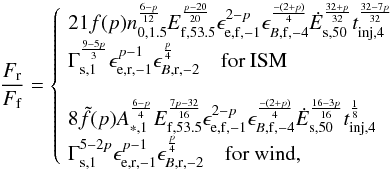 (25)where
  are numerical factors of order unity, depending weakly on p. Naturally, a large energy in the slow moving material as compared with that in the fast moving material and a higher density of the external medium lead to an increase in this ratio. Furthermore, as noted above, a small value of ϵB,f suppresses the synchrotron flux from the forward shock and therefore also increases this ratio.
6. Discussion and conclusions
GRB 070110 was a peculiar event. While its prompt phase was not remarkable, showing a few pulses and ending with the usual early steep decay of temporal index close to −3, it was followed by a very flat plateau interrupted by an extremely steep drop with the X-ray flux declining as t-9. One (or two) bump(s) were observed just after this drop with the flux increasing by a factor 2–3 before a more regular power-law decline of index −0.6 eventually followed until the end of XRT observations after three weeks.
We interpreted the initial early steep decay as the high latitude emission from the last flashing shell of the prompt phase. This implies a large emission radius for the prompt phase R ~ 2 cΓ2τ, where τ is the duration of the prompt activity and therefore favours dissipation from internal shocks or magnetic reconnection above the photosphere. For the plateau we first reconsidered the possibility that it could be powered by a magnetar but concluded that it was not likely due to tight constraints on the energy budget and a fine-tuning requiring the collapse to happen at a time just below the spin-down time of the magnetar.
We instead favour a scenario in which the plateau results from the photospheric emission of a continuous outflow of moderate Lorentz factor emitted from a central black hole, wherein the outflow is probably powered by accretion and the prompt phase of the outflow is powered by the Blandford-Znajek mechanism. The geometric timescale at the photospheric radius is then so short that the very steep decay at the end of the plateau is unlikely to be dominated by high-latitude emission from the photosphere, and rather, should correspond to the actual shutdown of the central source activity. Some dissipation must take place in the flow, both to increase the efficiency compared to a pure adiabatic evolution and to transform the original blackbody spectrum by adding a power-law tail at high energy.
The propagation of the reverse shock in the material producing the plateau generates a bump in the light curve since, owing to the assumed nearly uniform Lorentz factor, it is crossed by the shock in a short timescale. If, in addition, the outflow ends with a tail where the Lorentz factor decreases to values close to unity in a few hundreds of seconds, the reverse shock contribution will be long-lived and could account for the late shallow temporal slope in both the X-rays and visible wavelengths.
If this global picture is correct it leads to a certain number of consequences as follows:
-
The decay at the end of a period of activity can be used to con-strain the emission radius and therefore the dissipative pro-cess and radiation mechanism. In the case of GRB 070110,it predicts that the prompt phase resulted from dissipa-tion above the photosphere (from internal shocks or mag-netic reconnection), while the plateau phase was of photo-spheric origin. Photospheric emission during the promptphase was therefore subdominant, for example because theejecta was still magnetically dominated (see also Hascoëtet al. 2013). Conversely, dur-ing the plateau, dissipation was mostly confined below thephotosphere. This could be simply due to the increase of the pho-tospheric radius at low Lorentz factor (even if the injected powerdecreases). For example, in the case of shock dissipation, the ratioRIS/Rph ∝ Γ5 could easily fall below unity at low Γ.
-
If the bump following the plateau indeed results from the propagation of the reverse shock in the low Γ part of the ejecta, it shows that the magnetization was low (σ ≲ 0.1) at that time, either because it was originally low or has decreased during the propagation of the flow.
-
The peculiarities of GRB 070110, i.e. the internal plateau, very steep drop at the end of the plateau, and shallow decline at late times, are unusual. This could indicate that (i) a prolonged activity of the central engine is rare, or (ii) that plateaus, even if present, radiate mostly in UV because the Lorentz factor of the long-lasting outflow is lower than 10–20 or that they are dimmer owing to less injected power or to adiabatic cooling without additional dissipation in the outflow.
-
If other bursts with similar internal plateaus are found, we might be able to detect bumps and/or deviation from closure relations in their afterglow after the plateau. At present, only a few events with flat plateaus followed by a steep decline have been found, such as GRB 060413 or GRB 120213A. But the decay after the plateau is not as steep as in GRB 070110 (with a temporal index of −2.5 to −3), which does not necessarily require a photospheric origin.
-
More speculatively, one may postulate that the high density environment apparently implied by the bump and late-time afterglow is physically related to the prolonged activity of the central engine. This may happen, for instance, if due to a more violent mass ejection towards the end of the life of a star it ejected more matter that ended up being accreted to the newly formed black hole. This possibility may be quantitatively testable with numerical simulations or observationally if future GRBs reveal similar properties to those of GRB 070110.
The study of GRB 070110 illustrates how bursts with non-standard features can help decipher the dissipation processes and radiation processes at work in GRBs. Any indication of the presence of shocks constrains the magnetization. The variability timescales puts limits on the angular spreading and therefore on the emission radius. Finally, plateaus can be related to late source activity. One may hope that the diversity in early afterglow behaviours, which can be viewed as a source of confusion, may also provide tools for a better understanding of GRB physics.
One may tentatively propose that these two phases are powered by the extraction of the black-hole rotational energy via the Blandford-Znajek mechanism and by the release of gravitational energy from accretion, respectively.
In fact, even if the acceleration is more gradual, for example, Γ ∝ r1/3 as expected for MHD jets (Drenkhahn 2002), the observed temperature when acceleration is incomplete at the photosphere is still expected to be ~100 keV with a relatively weak dependence on the jet parameters (Giannios & Spruit 2005). This result can also be extended to generic acceleration models as shown by Giannios (2012).
The alternative possibility, that both bands are below the cooling break, would require rather irregular values of p > 3 and smaller values of ϵB for the emitting material.
Acknowledgments
We thank Johannes Buchner for applying the spectral fits to the plateau data using the Comptonized photospheric model as described in Sect. 4.2. We also thank the anonymous referee for their detailed comments and suggestions on the manuscript. P.B. is supported by a Chateaubriand Fellowship.
References
- Ackermann, M., Ajello, M., Allafort, A., et al. 2013, Science, 339, 807 [NASA ADS] [CrossRef] [PubMed] [Google Scholar]
- Axelsson, M., Baldini, L., Barbiellini, G., et al. 2012, ApJ, 757, L31 [NASA ADS] [CrossRef] [Google Scholar]
- Barniol Duran, R. 2014, MNRAS, 442, 3147 [NASA ADS] [CrossRef] [Google Scholar]
- Beloborodov, A. M. 2000, ApJ, 539, L25 [NASA ADS] [CrossRef] [Google Scholar]
- Beloborodov, A. M. 2010, MNRAS, 407, 1033 [NASA ADS] [CrossRef] [Google Scholar]
- Beloborodov, A. M. 2011, ApJ, 737, 68 [NASA ADS] [CrossRef] [Google Scholar]
- Beloborodov, A. M. 2013, ApJ, 764, 157 [NASA ADS] [CrossRef] [Google Scholar]
- Beniamini, P., & Giannios, D. 2017, MNRAS, 468, 3202 [NASA ADS] [CrossRef] [Google Scholar]
- Beniamini, P., & Granot, J. 2016, MNRAS, 459, 3635 [NASA ADS] [CrossRef] [Google Scholar]
- Beniamini, P., & Piran, T. 2013, ApJ, 769, 69 [NASA ADS] [CrossRef] [Google Scholar]
- Beniamini, P., & Piran, T. 2014, MNRAS, 445, 3892 [NASA ADS] [CrossRef] [Google Scholar]
- Beniamini, P., Guetta, D., Nakar, E., & Piran, T. 2011, MNRAS, 416, 3089 [NASA ADS] [CrossRef] [Google Scholar]
- Beniamini, P., Nava, L., Duran, R. B., & Piran, T. 2015, MNRAS, 454, 1073 [NASA ADS] [CrossRef] [Google Scholar]
- Beniamini, P., Nava, L., & Piran, T. 2016, MNRAS, 461, 51 [NASA ADS] [CrossRef] [Google Scholar]
- Bošnjak, Ž., Daigne, F., & Dubus, G. 2009, A&A, 498, 677 [NASA ADS] [CrossRef] [EDP Sciences] [Google Scholar]
- Burgess, J. M., Bégué, D., Ryde, F., et al. 2016, ApJ, 822, 63 [NASA ADS] [CrossRef] [Google Scholar]
- Daigne, F., & Mochkovitch, R. 1998, MNRAS, 296, 275 [NASA ADS] [CrossRef] [Google Scholar]
- Daigne, F., & Mochkovitch, R. 2000, A&A, 358, 1157 [NASA ADS] [Google Scholar]
- Daigne, F., Bošnjak, Ž., & Dubus, G. 2011, A&A, 526, A110 [NASA ADS] [CrossRef] [EDP Sciences] [Google Scholar]
- Drenkhahn, G. 2002, A&A, 387, 714 [NASA ADS] [CrossRef] [EDP Sciences] [Google Scholar]
- Drenkhahn, G., & Spruit, H. C. 2002, A&A, 391, 1141 [NASA ADS] [CrossRef] [EDP Sciences] [Google Scholar]
- Du, S., Lü, H.-J., Zhong, S.-Q., & Liang, E.-W. 2016, MNRAS, 462, 2990 [NASA ADS] [CrossRef] [Google Scholar]
- Fan, Y.-Z., Dai, Z.-G., Huang, Y.-F., & Lu, T. 2002, Chin. J. Astron. Astrophys., 2, 449 [NASA ADS] [CrossRef] [Google Scholar]
- Genet, F., Daigne, F., & Mochkovitch, R. 2007, MNRAS, 381, 732 [NASA ADS] [CrossRef] [Google Scholar]
- Ghisellini, G., & Celotti, A. 1999, ApJ, 511, L93 [NASA ADS] [CrossRef] [Google Scholar]
- Giannios, D. 2006, A&A, 457, 763 [NASA ADS] [CrossRef] [EDP Sciences] [Google Scholar]
- Giannios, D. 2008, A&A, 480, 305 [NASA ADS] [CrossRef] [EDP Sciences] [Google Scholar]
- Giannios, D. 2012, MNRAS, 422, 3092 [NASA ADS] [CrossRef] [Google Scholar]
- Giannios, D., & Spruit, H. C. 2005, A&A, 430, 1 [NASA ADS] [CrossRef] [EDP Sciences] [Google Scholar]
- Giannios, D., & Spruit, H. C. 2007, A&A, 469, 1 [NASA ADS] [CrossRef] [EDP Sciences] [Google Scholar]
- Granot, J. 2016, ApJ, 816, L20 [NASA ADS] [CrossRef] [Google Scholar]
- Granot, J., & Sari, R. 2002, ApJ, 568, 820 [NASA ADS] [CrossRef] [Google Scholar]
- Granot, J., Piran, T., Bromberg, O., Racusin, J. L., & Daigne, F. 2015, Space Sci. Rev., 191, 471 [NASA ADS] [CrossRef] [Google Scholar]
- Guetta, D., Pian, E., & Waxman, E. 2011, A&A, 525, A53 [NASA ADS] [CrossRef] [EDP Sciences] [Google Scholar]
- Guiriec, S., Connaughton, V., Briggs, M. S., et al. 2011, ApJ, 727, L33 [NASA ADS] [CrossRef] [Google Scholar]
- Hamil, O., Stone, J. R., Urbanec, M., & Urbancová, G. 2015, Phys. Rev. D, 91, 063007 [NASA ADS] [CrossRef] [Google Scholar]
- Hascoët, R., Daigne, F., & Mochkovitch, R. 2012, A&A, 542, L29 [NASA ADS] [CrossRef] [EDP Sciences] [Google Scholar]
- Hascoët, R., Daigne, F., & Mochkovitch, R. 2013, A&A, 551, A124 [NASA ADS] [CrossRef] [EDP Sciences] [Google Scholar]
- Kagan, D., Nakar, E., & Piran, T. 2016, ApJ, 826, 221 [NASA ADS] [CrossRef] [Google Scholar]
- Katz, J. I. 1994, ApJ, 432, L107 [NASA ADS] [CrossRef] [Google Scholar]
- Kobayashi, S., Piran, T., & Sari, R. 1997, ApJ, 490, 92 [NASA ADS] [CrossRef] [Google Scholar]
- Kobayashi, S., & Zhang, B. 2003, ApJ, 597, 455 [NASA ADS] [CrossRef] [Google Scholar]
- Kumar, P., & McMahon, E. 2008, MNRAS, 384, 33 [NASA ADS] [CrossRef] [Google Scholar]
- Kumar, P., & Piran, T. 2000, ApJ, 532, 286 [NASA ADS] [CrossRef] [Google Scholar]
- Kumar, P., & Zhang, B. 2015, Phys. Rep., 561, 1 [NASA ADS] [CrossRef] [Google Scholar]
- Lattimer, J. M., & Prakash, M. 2004, Science, 304, 536 [NASA ADS] [CrossRef] [PubMed] [Google Scholar]
- Lazzati, D., & Begelman, M. C. 2010, ApJ, 725, 1137 [NASA ADS] [CrossRef] [Google Scholar]
- Lemoine, M., Li, Z., & Wang, X.-Y. 2013, MNRAS, 435, 3009 [NASA ADS] [CrossRef] [Google Scholar]
- Levinson, A. 2012, ApJ, 756, 174 [NASA ADS] [CrossRef] [Google Scholar]
- Liang, E. W., Zhang, B., O’Brien, P. T., et al. 2006, ApJ, 646, 351 [NASA ADS] [CrossRef] [Google Scholar]
- Lyons, N., O’Brien, P. T., Zhang, B., et al. 2010, MNRAS, 402, 705 [NASA ADS] [CrossRef] [Google Scholar]
- McKinney, J. C., & Uzdensky, D. A. 2012, MNRAS, 419, 573 [Google Scholar]
- McMahon, E., Kumar, P., & Piran, T. 2006, MNRAS, 366, 575 [NASA ADS] [CrossRef] [Google Scholar]
- Mészáros, P., & Rees, M. J. 2000, ApJ, 530, 292 [NASA ADS] [CrossRef] [Google Scholar]
- Nakar, E., Ando, S., & Sari, R. 2009, ApJ, 703, 675 [NASA ADS] [CrossRef] [Google Scholar]
- Nava, L., Vianello, G., Omodei, N., et al. 2014, MNRAS, 443, 3578 [NASA ADS] [CrossRef] [Google Scholar]
- Pe’er, A., & Waxman, E. 2004, ApJ, 613, 448 [NASA ADS] [CrossRef] [Google Scholar]
- Pe’er, A., Mészáros, P., & Rees, M. J. 2005, ApJ, 635, 476 [NASA ADS] [CrossRef] [Google Scholar]
- Rees, M. J., & Meszaros, P. 1994, ApJ, 430, L93 [NASA ADS] [CrossRef] [Google Scholar]
- Rees, M. J., & Mészáros, P. 2005, ApJ, 628, 847 [NASA ADS] [CrossRef] [Google Scholar]
- Santana, R., Barniol Duran, R., & Kumar, P. 2014, ApJ, 785, 29 [NASA ADS] [CrossRef] [Google Scholar]
- Sari, R., & Esin, A. A. 2001, ApJ, 548, 787 [NASA ADS] [CrossRef] [Google Scholar]
- Sari, R., Narayan, R., & Piran, T. 1996, ApJ, 473, 204 [NASA ADS] [CrossRef] [Google Scholar]
- Shao, L., & Dai, Z. G. 2005, ApJ, 633, 1027 [NASA ADS] [CrossRef] [Google Scholar]
- Sironi, L., & Spitkovsky, A. 2011, ApJ, 726, 75 [NASA ADS] [CrossRef] [Google Scholar]
- Sironi, L., Petropoulou, M., & Giannios, D. 2015, MNRAS, 450, 183 [NASA ADS] [CrossRef] [Google Scholar]
- Swenson, C. A., Maxham, A., Roming, P. W. A., et al. 2010, ApJ, 718, L14 [NASA ADS] [CrossRef] [Google Scholar]
- Thompson, C. 1994, MNRAS, 270, 480 [NASA ADS] [CrossRef] [Google Scholar]
- Troja, E., Cusumano, G., O’Brien, P. T., et al. 2007, ApJ, 665, 599 [NASA ADS] [CrossRef] [Google Scholar]
- Uhm, Z. L., & Beloborodov, A. M. 2007, ApJ, 665, L93 [NASA ADS] [CrossRef] [Google Scholar]
- Usov, V. V. 1994, MNRAS, 267, 1035 [NASA ADS] [CrossRef] [Google Scholar]
- Vurm, I., Beloborodov, A. M., & Poutanen, J. 2011, ApJ, 738, 77 [NASA ADS] [CrossRef] [Google Scholar]
- Wang, X.-Y., Liu, R.-Y., & Lemoine, M. 2013, ApJ, 771, L33 [NASA ADS] [CrossRef] [Google Scholar]
- Yu, Y.-W., Cheng, K. S., & Cao, X.-F. 2010, ApJ, 715, 477 [NASA ADS] [CrossRef] [Google Scholar]
- Zhang, B., & Mészáros, P. 2001, ApJ, 552, L35 [NASA ADS] [CrossRef] [Google Scholar]
- Zhang, B., & Yan, H. 2011, ApJ, 726, 90 [NASA ADS] [CrossRef] [Google Scholar]
- Zhang, B., Fan, Y. Z., Dyks, J., et al. 2006, ApJ, 642, 354 [NASA ADS] [CrossRef] [Google Scholar]
- Zhang, B.-B., van Eerten, H., Burrows, D. N., et al. 2015, ApJ, 806, 15 [NASA ADS] [CrossRef] [Google Scholar]
All Figures
|
Fig. 1 Normalized luminosity (L/L0) as a function of time (see Eq. (3)) for various spin-down models (n = 1,2,3) as compared with the observed XRT data. We take t0 = 2 × 10⁴ s, which is the observed time of the end of the plateau, and ts = 4000 s, which is the observed time at which the plateau starts and is an upper limit on the actual value. |
| In the text | |
|
Fig. 2 Dissipated power as a function of time for a fast shell of material (Γ ≈ 200) that decelerates into the external medium and is eventually overtaken by a slower outflow, where Γ = 20. Results are shown for a uniform medium of density n = 30 cm-3 (red) and a stellar wind with A∗ = 2.4 (blue). |
| In the text | |
|
Fig. 3 Light-curves corresponding to reverse and forward shock emission assuming the ejecta responsible for the prompt emission is followed by slower moving outflow with Γs = 20, Ės = 2 × 1049 erg s-1 and lasting 6000 s, which makes the plateau. The tail of this material is characterized by the same Ė, lasting 400 s and with a declining Lorentz factor from Γ ≈ 20 down to Γ ≈ 1 with Γ(tinj) ∝ (tf−tinj)2/11. The reverse shock crossing this material accounts for a bump in the afterglow data. The time of the bump and the flux levels during and after the bump match the observed levels. We assume here A∗ = 2.2,ϵe,f = 0.1,ϵB,f = 2.5 × 10⁻⁵,ϵe,r = 0.1,ϵB,r = 4 × 10⁻³,p = 2.15. The top panels correspond to the 1 keV light curve and the bottom panels correspond to the 1 eV light curve. Left: light curve for the reverse shock (blue dot-dashed line) and forward shock (red dashed line). A yellow solid line depicts the sum of the reverse and forward shock contributions. Right: the plots show the evolution of νc,R (blue circles), νm,R (red pluses), νc,f (yellow dashed line) and νm,f (purple dot-dashed line). The observed frequency is depicted by a horizontal line. |
| In the text | |
|
Fig. 4 Same as Fig. 3 for an ISM medium with n0 = 30 cm-3. The choice of burst parameters is the same as in Fig. 3 except for ϵB,f = 10-4,ϵB,r = 2 × 10⁻². |
| In the text | |
Current usage metrics show cumulative count of Article Views (full-text article views including HTML views, PDF and ePub downloads, according to the available data) and Abstracts Views on Vision4Press platform.
Data correspond to usage on the plateform after 2015. The current usage metrics is available 48-96 hours after online publication and is updated daily on week days.
Initial download of the metrics may take a while.