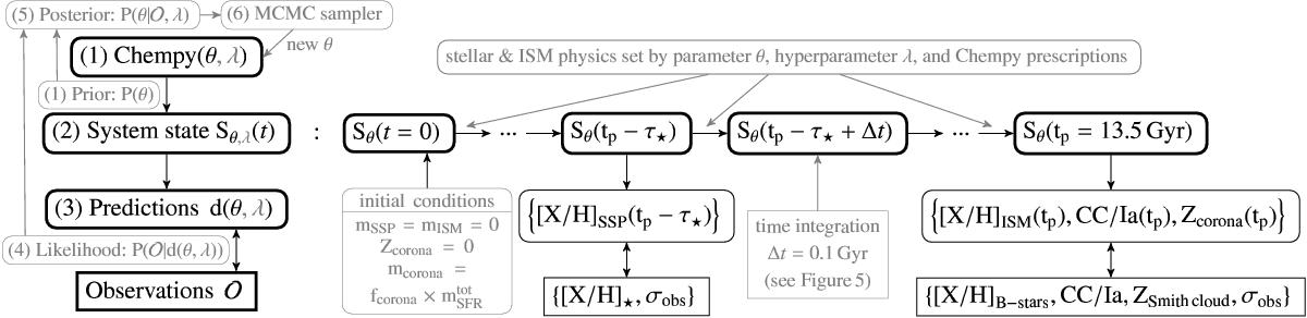
Schematic summary of Chempy: the left portion of this figure illustrates the sampling of the model parameter posteriors within the Bayesian framework (see Sect. 4); the right hand portion sketches how Chempy calculates a “system state”, for any one set of (hyper-)parameters, which produces observable predictions: (1) for a chosen set of parameters, θ, Chempy calculates the system state from initial conditions for all time steps (2, cf. Fig. 5), resulting in the observational predictions (3). These predictions are then compared to a predefined subset of our observations (see Table 3); here τ_⋆ is the age of the tracers, whose abundance measurements we fit. In our sample application, this is the age of the Sun or Arcturus. We can now calculate the likelihood (4) of any set of observations (, and their variances σ_obs). The posterior (5) is the result of multiplying the likelihood with the parameter priors (see Table 1). The model parameters’ posterior PDF can be sampled using an MCMC algorithm (6). An example of a converged MCMC run can be seen in Fig. 12, where the prior distribution over the parameter space is displayed for comparison.