| Issue |
A&A
Volume 604, August 2017
|
|
|---|---|---|
| Article Number | A39 | |
| Number of page(s) | 9 | |
| Section | Stellar structure and evolution | |
| DOI | https://doi.org/10.1051/0004-6361/201630060 | |
| Published online | 31 July 2017 | |
Gamma rays from clumpy wind-jet interactions in high-mass microquasars
1 Departament de Física Quàntica i Astrofísica, Institut de Ciènces del Cosmos (ICCUB), Universitat de Barcelona (IEEC-UB), Martí i Franquès 1, 08028 Barcelona, Spain
e-mail: vmdelacita@fqa.ub.edu
2 Instituto Argentino de Radioastronomía (CCT La Plata, CONICET), C.C.5, (1894) Villa Elisa, Buenos Aires, Argentina
3 Facultad de Ciencias Astronómicas y Geofísicas, Universidad Nacional de La Plata, Paseo del Bosque, 1900 FWA La Plata, Argentina
4 Department of Physics, Rikkyo University 3-34-1, Nishi-Ikebukuro, Toshima-ku, 171-8501 Tokyo, Japan
Received: 14 November 2016
Accepted: 18 January 2017
Context. The stellar winds of the massive stars in high-mass microquasars are thought to be inhomogeneous. The interaction of these inhomogeneities, or clumps, with the jets of these objects may be a major factor in gamma-ray production.
Aims. Our goal is to characterize a typical scenario of clump-jet interaction, and calculate the contribution of these interactions to the gamma-ray emission from these systems.
Methods. We use axisymmetric, relativistic hydrodynamical simulations to model the emitting flow in a typical clump-jet interaction. Using the simulation results we perform a numerical calculation of the high-energy emission from one of these interactions. The radiative calculations are performed for relativistic electrons locally accelerated at the jet shock, and the synchrotron and inverse Compton radiation spectra are computed for different stages of the shocked clump evolution. We also explore different parameter values, such as viewing angle and magnetic field strength. The results derived from one clump-jet interaction are generalized phenomenologically to multiple interactions under different wind models, estimating the clump-jet interaction rates, and the resulting luminosities in the GeV range.
Results. If particles are efficiently accelerated in clump-jet interactions, the apparent gamma-ray luminosity through inverse Compton scattering with the stellar photons can be significant even for rather strong magnetic fields and thus efficient synchrotron cooling. Moreover, despite the standing nature or slow motion of the jet shocks for most of the interaction stage, Doppler boosting in the postshock flow is relevant even for mildly relativistic jets.
Conclusions. For clump-to-average wind density contrasts greater than or equal to ten, clump-jet interactions could be bright enough to match the observed GeV luminosity in Cyg X-1 and Cyg X-3 when a jet is present in these sources, with required non-thermal-to-total available power fractions greater than 0.01 and 0.1, respectively.
Key words: binaries: general / accretion, accretion disks / stars: early-type / X-rays: binaries / acceleration of particles / gamma rays: stars
© ESO, 2017
1. Introduction
High-mass microquasars (HMMQs) are binary systems hosting both a massive star and a compact object that are able to produce jets in which high-energy (HE) processes can take place (see, e.g., Bosch-Ramon & Khangulyan 2009; Dubus 2013; Bednarek 2013, and references therein). To date, gamma rays have been robustly detected from two HMMQs, Cyg X-3 and Cyg X-1 (Tavani et al. 2009; Zanin et al. 2016, respectively). Variability of the detected emission indicates that the high-energy source should be located relatively close to the compact object, at a distance comparable to the binary separation distance (Dubus et al. 2010b; Zanin et al. 2016). There is a tentative detection of another HMMQ, SS 433, although in this case the emission would be likely coming from the jet-termination region (Bordas et al. 2015).
The energies at which Cyg X-1 and Cyg X-3 were detected are in the GeV range, except for a flare-like detection of Cyg X-1 with the MAGIC Cherenkov telescope in the TeV range with post-trial significance of 4.1σ (Albert et al. 2007). Both sources present long-term gamma-ray emission, overlapping with possible day-scale flares, all associated with jet activity (Albert et al. 2007; Tavani et al. 2009; Fermi LAT Collaboration et al. 2009; Sabatini et al. 2010; Malyshev et al. 2013; Bodaghee et al. 2013; Zanin et al. 2016; Zdziarski et al. 2016b,a). In what follows, we will take a mixed approach that considers HMMQs in general, whilst adopting Cyg X-1 and Cyg X-3 as reference sources to check our results in the context of real objects.
Massive stars produce dense and fast winds that are thought to be inhomogeneous (e.g. Runacres & Owocki 2002; Moffat 2008; Puls et al. 2008, and references therein). The specific properties of these inhomogeneous winds may depend on the stellar type and evolutionary phase, but in general they can be described in terms of dense clumps in a dilute medium. In particular, Cyg X-1 hosts a black hole and an O-type supergiant, and Cyg X-3 either a neutron star or a black hole, and a Wolf-Rayet (WR) star. Clumpy winds have been suggested to be present in both systems (see, e.g. Szostek & Zdziarski 2008; Rahoui et al. 2011; Miškovičová et al. 2016).
Detection of gamma-ray emission from galactic jet sources requires efficient particle acceleration, which is conventionally associated with shocks. The propagation of a jet through the binary system environment may happen simultaneously with the formation of shocks at binary scales in addition to the jet termination shock. For example, internal shocks form when portions of jet material, moving with different velocities, collide with each other (e.g. Bosch-Ramon et al. 2006). Furthermore, the stellar wind lateral impact should produce asymmetric recollimation shocks and induce non-thermal emission (e.g. Romero et al. 2003; Perucho & Bosch-Ramon 2008; Dubus et al. 2010a; Yoon et al. 2016). However, it cannot be neglected that when wind density inhomogeneities or clumps penetrate inside the jets, they should trigger strong shocks as well. Thus, the wind clumps in HMMQs may have a significant influence on the jet dynamics (Perucho & Bosch-Ramon 2012) and on the non-thermal HE processes occurring on the scales of the binary system (Owocki et al. 2009; Araudo et al. 2009; Romero et al. 2010). Therefore, although all these types of shocks can be sites of efficient particle acceleration and HE emission, one expects the strongest kinetic-to-internal energy conversion for those shocks associated with wind clumps present inside the jet (Bosch-Ramon 2015). Moreover, besides this high-conversion efficiency, the Doppler boosting of the non-thermal emission associated with wind clumps, in addition to being important, might also be favourable for relatively off-axis observers.
In this work, we present for the first time numerical calculations of the HE emission produced by a clump-jet interaction in a HMMQ using the hydrodynamical information obtained from a simplified relativistic, hydrodynamical (RHD) axi-symmetric simulation of such an interaction. Particle acceleration is assumed to occur in the jet shock, because this is much more energetic than the shock initially crossing the clump. The parameters adopted have been chosen such that the simulation can be taken as a reference case, meaning that we have studied a clump of realistic parameters inside the jet at a typical interaction jet height, similar to the binary size. Interactions taking place significantly closer or farther from the jet base would be either very unlikely or too oblique for the clump to penetrate into the jet (Eq. (1)). Therefore, the calculations performed can be used as a reference to establish the typical radiation outcome from one interaction, having choosen a suitable orbital phase, although some of the results have been checked for different orbital phases. The radiation results can be then generalized to the realistic case of multiple wind clumps interacting with the jet, adopting a phenomenological prescription for the inhomogeneous wind properties, similar to what was done in Bosch-Ramon (2013) in the context of a high-mass binary hosting a young pulsar.
The paper is organized as follows. In Sect. 2, the conditions under which a clump is able to penetrate into a jet are computed. Then, in Sect. 3 we first briefly introduce the results of a simplified RHD axi-symmetric simulation of a characteristic clump-jet interaction, and the streamline approach to define the emitter structure. We then introduce the non-thermal radiation calculations and their results. In Sect. 4, a generalization of the numerical radiation results is carried out adopting a phenomenological prescription for the clumpy wind properties. Finally, a discussion of the obtained results in the context of the HMMQs Cyg X-1 and Cyg X-3 is presented in Sect. 5, along with a summary of the conclusions of the work.
2. Clump-jet interaction: basic estimates
In this section we analyse the main characteristics of a clump-jet interaction, and show that even for conservative assumptions it is likely that clumps penetrate the jet. The following quantities are required for the analysis: (i) the stellar mass-loss rate (Ṁw), wind velocity (vw), and wind density (ρw); (ii) the jet luminosity (without accounting for the rest-mass energy Lj), velocity (vj, or Lorentz factor Γj), radius (Rj), height (zj), density (ρj), and jet half opening angle (θj = Rj/zj); (iii) the clump characteristic radius (Rc) and density (ρc) (assuming spherical uniform clumps), the latter of which relates to the average wind density through the density contrast or clumping factor (χ = ρc/ρw > 1); and finally (iv) the distance between the star and the base of the jet, or orbital separation distance (Rorb). In this work, the jet is assumed to be perpendicular to the orbital plane. We also considered a mildly relativistic jet (see Sect. 2 in Bosch-Ramon & Barkov 2016), with Γj = 2. The hydrodynamic approximation for the clump-jet interaction was adopted, because the gyroradii of the particles involved are much smaller than the typical size of the interacting structures.
We considered the emission of a clump interacting with the jet at a distance from the jet base similar to Rorb. On these scales, clump-jet interactions are more numerous because the jet is thicker; the jet is also more dilute than further upstream, and the clump velocity is still rather perpendicular to the jet, favouring jet penetration. Moreover, at smaller distances from the compact object the jet ram pressure is too strong for the clumps to survive penetration. For high density contrast values, such as χ ≫ 1, wind-jet interactions may occur just through clumps entering into the jet. In that case, the clumps would be surrounded by a very dilute, hot medium of little dynamical impact either for the jet, or the clumps. However, we herein adopt the more conservative assumption that, even if χ ~ 10, the wind interacts with the jet forming a relatively smooth region of shocked material that circumvents the jet (Perucho & Bosch-Ramon 2012 and also Pittard 2007 in the context of colliding wind binaries). This shocked wind can prevent small clumps from reaching the jet, which sets the first condition for clump-jet interaction to occur. Moreover, the impact of the jet upon a clump generates a shock that propagates in the latter and eventually destroys it. Therefore a second condition is that the forward shock in the clump is slower than the clump velocity perpendicular to the jet; this allows the clump to enter deep enough into the jet before its destruction (see, e.g. Araudo et al. 2009).
To formalize the first condition, let us consider a clump that travels with a velocity of approximately vw perpendicular to the jet and reaches the region where the wind interacts with the jet boundary. To successfully penetrate the jet, the clump has to go through the shocked wind, with respect to which the clump is moving also at approximately vw, without significantly slowing down. Such a region has a thickness of approximately Rj and exerts a drag on the clump that can be quantified through a ram pressure  . The acceleration exerted on the clump, which has a characteristic surface
  and volume Vc ≈ 4/3 scRc ≈ scRc, by this pressure is aacc ≈ scPw/mc. Using mc = Vcρc, Vc/sc ≈ Rc, and ρc = χρw, one can obtain the expression aacc ≈ Pw/ (χρwRc). Therefore, the typical distance required to significantly slow down the clump in the shocked wind surrounding the jet is
  . As noted above l ≳ Rj, and therefore Rc ≳ Rj/χ setting a lower limit on the clump size:
  (1)The second condition for clumps to fully penetrate into the jet at zj ≲ Rorb is vsh ≲ vw1, where vsh is the velocity of the shock produced within the clump by the jet impact. For a cold jet, its pressure Pj is dominated by the kinetic component of the momentum flux as described by
  . Assuming equilibrium between the jet ram pressure and shocked clump pressure, we obtain vsh ≈ (Pj/ρc)1/2 ≈ Γj(ρj/ρc)1/2vj. Considering that
  and fixing zj ~ Rorb, i. e. Rj ~ θjRorb, one gets the following limitation for the jet power:
  (4)For a hot jet, the specific enthalpy should be included to derive Pj.
For the typical parameters of Cyg X-3 and Cyg X-1 (see Yoon et al. 2016; Bosch-Ramon & Barkov 2016, and references therein), and adopting χ ~ 10 and Γj ~ 2, clumps will be able to penetrate into the jets of these HMMQ for Rc ~ 3 × 10⁹ and Lj ≲ 1038, and 3 × 1010 cm and 1037 erg s-1. These jet powers are actually similar to the values estimated for these sources, although the uncertainties in the clumpy wind and the jet properties are large.
3. Clump-jet interaction: numerical calculations
3.1. Hydrodynamics
 |
Fig. 1 Density maps of the clump-jet interaction simulation that illustrate the clump evolution after ~ 73, 521, 596, 708, and 822 s (or, equivalently, to approximately 0.5, 3.5, 4.1, 4.8, and 5.6 in Rc/vsh units). |
The clump-jet interaction was simulated in two dimensions (2D) assuming axisymmetry, in other words neglecting the clump motion with respect to, for example, the compact object frame and a dynamically negligible magnetic field. An adiabatic gas with constant index  was assumed2. The RHD equations were solved using the Marquina flux formula (Donat & Marquina 1996; Donat et al. 1998). The code is the same as the one used in Bosch-Ramon (2015), but the spatial reconstruction scheme has been improved from second to third order applying the piecewise parabolic method reconstruction scheme (Colella & Woodward 1984; Martí & Müller 1996; Mignone et al. 2005).
The resolution of the calculations was 300 cells in the vertical direction, the z-axis, and 150 in the radial direction, the r-axis. The physical size was  cm in the z-direction, and
  cm in the r-direction. This resolution was chosen such that no significant differences could be seen in the hydrodynamical results when going to higher resolution simulations. Inflow conditions (the jet) were imposed at the bottom of the grid, reflection at the axis, and outflow in the remaining grid boundaries. On the scales of the grid, for simplicity we approximated the jet streamlines at injection as oriented along the z-direction despite the jet is actually assumed to be conical.
The injected jet power without accounting for the jet rest-mass energy was ~ 2.3 × 1037 erg s-1 for the whole grid, up to  , with a Lorentz factor Γj = 2. The initial clump radius was Rc = 3 × 1010 cm, and its density ρc ~ 5 × 10-14 g cm-3. This density would correspond to that of a clump located at zj ~ 3 × 1012 cm, for a stellar wind with Ṁ ~ 3 × 10⁻⁶M⊙ yr-1, vw ~ 2 × 108 cm s-1, and χ ~ 10 (plus Rorb = 3 × 1012 cm). The initial clump location in the grid was (0,1011 cm).
After the jet impact, the clump gets shocked, expands, disrupts, and eventually leaves the grid (see, e.g., Bosch-Ramon 2012, in the context of extragalactic jets). The whole duration of the simulation was ~ 820 s. Five snapshots of the density distribution, illustrating the clump evolution after ~ 73, 521, 596, 708, and 822 s, are presented in Fig. 1. The shocked jet material forms a sort of cometary tail pointing upwards and surrounding the clump shocked material.
The grid size was chosen such that the simulation captured the first stages of the clump-jet interaction. This was enough to compute the non-thermal emission for two typical instances of the shocked clump evolution: (i) a quasi-stationary shock in the jet flow is present, but the clump has not expanded, nor it has been displaced, due to the jet impact; and (ii) the clump has already expanded, disrupted, and moved along the jet axis. A simulation with a significantly larger computational grid, and a much longer simulated time, is required for an accurate description of the clump-jet interaction until the clump has reached an asymptotic speed and probably fully fragmented and spread in the jet, in other words when no shock is present in the jet flow or it is much weaker. This should not affect the high-energy emission predictions qualitatively, but quantitative differences are expected. An accurate study of clump-jet mixing, lightcurves, and other factors is left for future work. The presence of the magnetic field, or 3D calculations, are likely to introduce further complexity to the problem through effects on the growth of instabilities such as suppression, anisotropy, or enhancement. These effects should be thoroughly studied through devoted simulations, which are out of the scope of the present work and left for the future. Future work may also include other effects for accuracy, such as a more realistic equation of state, or the back-reaction effects of non-thermal processes in the (magneto)hydrodynamics.
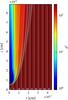 |
Fig. 2 Doppler boosting factor for φobs = 0°. The grey lines represent the computed streamlines, which are numbered. |
3.2. Streamlines
To compute the injection, evolution, and radiation of the non-thermal particles, the shocked jet flow was modelled as a set of streamlines, each divided in several cells. These streamlines correspond to the trajectory followed by a fluid element in the flow, which was assumed to be stationary. The assumption of stationarity for the shocked jet flow is valid because the dynamical time of the clump-jet interaction is much longer than the grid crossing time of this flow. The details of the streamline properties are described in de la Cita et al. (2016), Appendix A. The distribution of the streamlines in the radial direction in the present calculations is illustrated in Fig. 2.
Only streamlines injected at zgrid = 0 and rgrid ≤ 3 × 1011 cm were considered for radiation calculations. The reason was that the jet radius at the interaction location was assumed to be Rj = 3 × 1011 cm, which is equivalent to adopting a jet interaction height at zj ≈ Rorb and a half opening angle θj ~ 0.1 rad. However, the actual jet flow injection in the computational grid takes place up to in the r-axis. This was done for simplicity, because the actual jet surroundings may be very complex because of stellar wind presence and wind-jet interaction asymmetry. Thus, introducing a jet boundary in the hydrodynamical simulation seemed to us somewhat artificial if its conditions could not be set realistically. The total injected power in the streamlines was computed without taking into account the jet rest-mass energy, meaning within Rj = 3×1011 cm, results in ~ 1037 erg s-1.
Given the cylindrical symmetry of the simulation, each one of the cells in which the streamlines are divided represents an annular element of fluid in terms of volume and therefore energy content. However, from the point of view of particle energy evolution, propagation, and radiation, the cells are to be treated as point-like, because all these processes are not symmetric with respect to the jet axis. To mimic the 3D structure of the whole emitter, we assigned a random azimuthal angle ψ to each streamline when computing radiation, letting it vary from 0 to 2π radians to cover all the orientations (see de la Cita et al. 2016).
3.3. Non-thermal radiation computation
We needed the fluid information for each cell in each streamline to compute where and how much non-thermal particle energy is injected in the flow, and the evolution of the injected particles and later the inverse Compton (IC) and synchrotron radiation. We neglected at this point hadronic processes and relativistic Bremsstrahlung, because synchrotron and IC are in general far more efficient in terms of radiated energy (see, e.g., Bosch-Ramon & Khangulyan 2009). Each streamline was divided in 200 cells, enough to properly sample the flow, with a number of parameters: position and velocity vectors, pressure (P), density (ρ), section (S), magnetic field (B), and the fluid velocity divergence ( div(Γv) ), needed for the computation of adiabatic losses. For simplicity, the B-value in the fluid frame (FF) was computed assuming it is perpendicular to the flow velocity and that a fraction χB of the total flow-energy flux is in the form of Poynting flux (de la Cita et al. 2016). Two values were adopted: χB = 10-3 and 1. We note that the latter value is formally inconsistent with the hydrodynamical assumption of the simulations, but we still consider this case useful, because it sets an approximate lower limit on the IC with respect to the synchrotron emission.
For each streamline we followed the same procedure: we identified along the line where the internal energy increased and the fluid velocity decreased. In these cells we assumed there was a shock and therefore non-thermal particles were being injected, with a total energy corresponding to a fraction ηNT = 0.1 of the internal energy increment. We note that there is no feedback of the non-thermal population on the hydrodynamics, meaning we adopted a test particle approximation, and therefore the luminosity is linearly scalable with ηNT (incidentally, ηNT = 1 is consistent with , but in this case the test-particle approximation fails for a radiatively efficient emitter). The particles were assumed to be injected with an energy distribution following a power-law of index −2, typical for shock acceleration; and with two cutoffs, one at high energies that was derived assuming particle acceleration in a non-relativistic shock under Bohm diffusion (e.g. Drury 1983; de la Cita et al. 2016), and one at low energies. A significantly steeper power-law can be considered as another form of inefficiently accelerating high-energy emitting particles that is equivalent to a small ηNT-value. The low-energy cutoff was fixed to 1 MeV for simplicity, although our results are not very sensitive to this choice unless the low-energy cutoff is close to the energies of electrons emitting X-rays (mainly synchrotron) and gamma rays (mainly IC). Otherwise, only the normalization of the radiation spectrum would be slightly different.
Once the injection of non-thermal particles was known, we let them evolve and propagate through the streamlines until they left the simulation grid, at which point a steady-state was reached. The obtained energy distributions of the non-thermal particles for two B cases, low and high, are shown in Fig. 3. Once the non-thermal population was characterized, one could compute the IC and synchrotron radiation in the FF, and later transform the spectral energy distribution (SED) of this radiation to the observer frame. For that, we multiplied the photon energy by δ = 1/Γ [1−νcos(φobs)] and the SED by δ4, where φobs is the angle between the flow motion and the line of sight. The distribution of δ4 in the grid when adopting the most favourable case for detection (φobs = 0), is shown in Fig. 2.
We note that in the low magnetic field case, the highest energy particles could actually cross several streamlines before cooling significantly, despite still being confined to the interaction structure. This may affect the highest energy part of the spectrum to some extent, but for simplicity we assume that all electrons are attached to their respective streamlines because the bulk of the gamma-ray emission is radiated consistently with this assumption.
3.4. Radiation results
For simplicity in the following, we considered the radiation results for a typical orbital phase. We assumed a circular orbit and considered an orbital phase right in the middle between inferior and superior conjunction, in other words with the compact object in the plane of the sky. This provided a sort of typical high-energy SED. A more detailed analysis of the overall spectra in the different explored cases, and for different orbital phases, was out of the scope of the paper, as we were interested here in the average behaviour when the jet is present. We were also mostly interested in the 0.1–100 GeV band luminosity because this band is not strongly sensitive to parameters such as the maximum particle energy, and reacts smoothly to magnetic field and system-observer orientation changes. In contrast, the TeV band is very sensitive to all of these factors through IC effects and gamma-ray absorption (e.g. Bosch-Ramon & Khangulyan 2009, gamma-ray absorption is included in the present work). Furthermore, GeV luminosity is available for Cyg X-1 and Cyg X-3, because these sources have been detected in this energy band. For low-to-moderate B-values, the GeV band is also a good proxy for the source energetics and, unlike X-rays, is certainly of non-thermal nature.
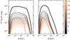 |
Fig. 3 Compression-phase electron energy distribution for the individual streamlines (thin lines), and the total electron distribution (thick lines). Left panel: low magnetic field case (χB = 10-3). Right panel: high magnetic field case (χB = 1). |
Two illustrative stages of the clump evolution were considered when presenting the results of our computations: (i) the first stage, when the clump is compressed by the jet ram pressure (hereafter called compression phase), the longest and more stable phase of the clump evolution; and (ii) a later, shorter stage when the clump is disrupted (hereafter called disruption phase), presenting a larger shock and therefore higher non-thermal emission. Both stages are shown in Fig. 1, first and third panels starting from the left. We also present in Fig. 4 the SEDs of all five snapshots of the hydrodynamical flow shown in Fig. 1, which illustrate how the high-energy emission varies with the clump evolution. The disruption phase was chosen as the maximum luminosity snapshot among those computed (i.e. snapshot 3). From the point of view of the hydrodynamics, snapshot 4 is characterized by a largest cross-section of the shocked jet, but the apparent non-thermal luminosity is higher for the hydrodynamic configuration shown in snapshot 3. This is likely related to a reduced Doppler boosting caused by stronger streamline deflection in snapshot 4 and perhaps additional weakening of the emission caused by the limited grid size.
In the three panels of Fig. 5, we focus first on the compression phase and varied B, and then we compare the compression and disruption phases. It can be seen that, in the case of a weak magnetic field, the transition from the compression to the disruption phase is accompanied by a flux increase by a factor of approximately five. In the high B case, the emission enhancement is modest, within a factor of two.
To illustrate the importance of the radiation losses, we compared the energy injected per time unit in the form of non-thermal particles with the energy of the particles leaving the computational grid, after suffering energy losses, in the laboratory frame. For the compression phase, the total injected luminosity is ~ 1.6×1035 (ηNT/ 0.1) erg s-1. About 33% of the energy is kept by the particles when leaving the grid in the low B case, being this percentage smaller (~ 15%) for the high B case. In the compression phase particles lose a ~ 49% of the injected energy through adiabatic losses, equating to ~ 7.7×1034 erg s-1. The synchrotron+IC losses are ~ 19% of the injected energy in the low B case, equating to ~ 3×1034 erg s-1 (~ 36% and ~ 5.8×1034 erg s-1 in the high B case). In the disruption phase, the total injected luminosity is ~ 1036 (ηNT/ 0.1) erg s-1. In that stage, particles gain energy through adiabatic heating because in some streamlines the flow is compressed, approximately 2×1035 erg s-1 (~ 20% of the injected energy). The synchrotron+IC losses are ~ 50% of the injected energy in the low B case, equating to ~ 5×1035 erg s-1 (~ 95% and ~ 9.5×1035 erg s-1 in the high B case). For the sake of discussion (Sect. 5), we provide in Table 1 the integrated luminosity in the range 0.1–100 GeV for the different cases studied here: the compression and disruption phases; the low and the high B cases; and φobs = 30°, given that this observing angle may be representative of both Cyg X-1 and Cyg X-3.
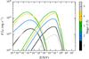 |
Fig. 4 Spectral energy distributions for the five stages shown in Fig. 1. Stage 1 corresponds to the compression phase, whereas stage 3 is the disruption phase; χB = 10-3 is adopted, and φobs = 30°. |
Values of the integrated emission in the 0.1–100 GeV band, given in erg s-1, considering an observer angle of φobs = 30°.
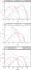 |
Fig. 5 Top panel: synchrotron and IC SEDs for the compression phase φobs = 0, 30, and 90°, and χB = 10-3. The thin lines represent the emission without taking into account gamma-ray absorption due to electron-positron pair creation, i.e. the production SED. Middle panel: the same as for the top panel but for χB = 1. Bottom panel: a comparison between the SEDs of the compression and disruption phases. |
4. Collective effects of a clumpy wind
Clumping is universal in massive star winds: these winds are stochastically inhomogeneous, believed to be composed of a hierarchy of clumps, with a few large ones and increasingly many more small ones, being the clump size and mass distributed as a power-law (Moffat & Corcoran 2009). The X-ray spectrum of single and binary massive stars is compatible with this picture of dominant small-scale clumps and rarer large clumps (Moffat 2008).
For simplicity, we considered the clumps to be spherical and neglected vorosity (i.e. porosity in velocity space, see e.g. Muijres et al. 2011), which in the present context can be considered as a minor effect. An empirical number density distribution of clumps with radius Rc was adopted: (5)with clump radii ranging Rc,min<Rc<Rc,max. The value of Rc,min could be considered close to the Sobolev length, RSob ≈ 0.01 R∗ (e.g. Owocki & Cohen 2006), while the clump size was at most of the order of R∗ (Liermann et al. 2010), although it may be significantly smaller. As clumps propagated from the region where they formed, at ~ 1−2 R∗ from the star centre, they could grow linearly with the stellar distance or somewhat slower for a slab geometry, but they could be also broken down by instabilities (see the discussion at the end of Sect. 3.3 in Bosch-Ramon 2013).
Assuming that all clumps have the same density and that the inter-clump medium is void, the clump volume filling factor is simply f = χ-1 (e.g. Hamann et al. 2008), and the distribution function should meet the following normalization condition:  (6)Fixing Rc,min = 0.01 R∗ and Rc,max = 0.5 R∗, we solved Eq. (6)to obtain the normalization constant n0.
Whether clump-jet interactions appear as a transient or as a persistent phenomenon is determined by the duty-cycle (DC) of these events. To determine DC we need to estimate the jet penetration rate of the clumps, Ṅ, and their lifetime, tc (Bosch-Ramon 2013). The jet crossing time will be more relevant than tc for jet powers Rc/Rj times the limit provided in Eq. (4). In this work we were interested in bright sources, and therefore the jet power was assumed to be close to the limit provided in Eq. (4). In fact, this is likely the case in the powerful jet sources Cyg X-3 and Cyg X-1.
The jet subtends a certain solid angle, Ω, as seen from the optical star. To interact with the jet, a clump must propagate within this solid angle. Considering a conical jet with Rj = θjzj and that the clump enters the jet roughly between 0.5Rorb ≲ z ≲ 1.5Rorb (so Δz ≈ Rorb), we obtained Ω ≈ θj/ 2 = 0.05. The differential rate of arrival to the jet for clumps of radius Rc could be estimated as dṄ = Ωd2vwn(Rc)dRc, where for simplicity  . The differential DC for those clumps is dDC = tcdṄ, with tc ≈ Rc/vsh, which we approximated here to tc = Rc/vw because we dealt with powerful jets3. From all this, the following estimate for the arrival of clumps with radius between R1 and R2 could be obtained:
 (7)We explored different values of the power-law index:
  . Values of α ≥ 4 imply that small clumps dominate the wind mass. Interestingly, because the energy emitted by one clump-jet interaction is expected to be proportional to tc×
 , one also obtains that for α> 3 the non-thermal radiation will be dominated by the smallest clumps that can enter into the jet, meaning those with Rc ~ R0. On the other hand, values of α ~ 2.5 are in accordance with the values inferred for WR stars (Moffat 2008)4.
The non-thermal luminosity of the clump-jet collective interactions depends on the dominant clump size; gamma rays can be mostly produced by small or large clumps. The DC may be dominated by small clumps, whilst the luminosity may be dominated by the largest ones. Nevertheless, the simulations show that clumps significantly larger than R0 cannot increase the luminosity output considerably and may even radiate less than smaller clumps interacting with the jet. The reason is that, unless (θj/ 0.1)(10 /χ) is well below one (Eq. (1)), larger clumps will likely disrupt the whole jet, strongly reduce the effect of Doppler boosting, and might even switch off particle acceleration. For the parameters adopted in this work, it seemed therefore natural to consider clumps of radii between approximately R0 and few times larger.
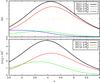 |
Fig. 6 Top panel: duty-cycle in the radius ranges 1−2 R0, 2−3 R0, 1−3 R0, and > 3 R0 for a wind clump number distribution n ∝ Rc− α. A value α ~ 5 represents a wind dominated by small clumps, whereas α2 ~ 2.5 is an observational value for Wolf-Rayet (WR) stars; R0 is the minimum clump size given by Eq. (1). Bottom panel: duty-cycle weighted by the effective section of the shock, and therefore its potential luminosity, shown in units of the luminosity L0 produced in the interaction of one clump of R = R0 with the jet. The case > 3 R0 is not shown as it may imply jet disruption. |
The top panel of Fig. 6 shows the DC dependence on α, whereas the bottom panel shows the DC dependence on the average luminosity of the collective clump-jet interactions. We focused on 1 R0<Rc< 3 R0, splitting this range into 1 R0<Rc< 2 R0 and 2 R0<Rc< 3 R0, although a curve for Rc> 3 R0 is also shown. The radius 3 R0 was considered as the upper-limit for the clumps to be relevant from the radiation point of view in the context of this work, that is (θj/ 0.1)(10 /χ) ~ 1. The results obtained allow the derivation of a rather robust conclusion, namely that clumps with Rc>R0 will be always present inside the jet unless the α parameters deviate strongly from the expected values. Also, the averaged total luminosity should be a factor of a few larger than the estimate obtained for a jet interacting with one clump of radius R0 (again unless α is in the extremes of the explored range). We studied cases with different Rc,max-values (not shown here), and found that our conclusions hold for a wide range of Rc,max ≈ 0.1−1 R∗.
For jet powers well below the value given in Eq. (4), the clump-jet interaction luminosity is proportional to Lj and therefore lower than the reference case, but the event duration is longer in proportion to  and
and  (vsh must be used instead of vw, as above). Thus, to first order, the decrease in the radiation luminosity will effectively be proportional to
  , although a more accurate relation should be derived numerically.
If clumps with Rc> 3 R0 are present and DC ≳ 0.5, the jet will likely be disrupted most of the time in the region of interest, zj ≈ Rorb. As noted, this is expected to significantly reduce the effects of Doppler boosting, and potentially might even switch off particle acceleration. In the scenario explored, namely (θj/ 0.1)(10 /χ) ~ 1, a value DC ≈ 0.5 for Rc> 3 R0 will be achieved only for α ≲ 3 and Rc,max ≈ 0.2 R∗. This sets limits on the wind parameters that allow clump-jet interactions to produce significant gamma-ray emission. These wind parameters are however somewhat extreme and possibly unrealistic, in particular the constraint on α, because in that case the wind mass would be dominated by the largest clumps.
Finally, we explore two situations different from (θj/ 0.1)(10 /χ) ~ 1:
Fixing (θj/ 0.1) ~ 1. Sources with (10 /χ) > 1 would imply that R0 would be larger andthat there may be no clumps big enough to cross the shocked windsurrounding the jet. In addition, a χ well below ten would meana rather homogeneous wind. On the other hand, for (10 /χ) < 1, R0 would besmaller and all the clumps may be able to reach the jet, and may bedense enough to fully enter inside. This would have the disruptingeffect of a wind with most of its mass in large, penetrating clumps(this kind of scenario is simulated in Perucho &Bosch-Ramon 2012). Additionally, the numberof clumps would be lower by χ-1 ∝ f (Eq. (6)), but because tcis actually proportional to f− 1/2 ∝ χ1/2, the radiation luminosity would beproportional to f1/2 ∝ χ− 1/2 lower.
Fixing (10 /χ) ~ 1. Taking (θj/ 0.1) < 1 would imply that smaller clumps could reach the jet, but the jet would be denser, making clump penetration more difficult and less frequent (DC ∝ Ω ∝ θj). On the other hand, if (θj/ 0.1) > 1, jet penetration would be significantly easier and more frequent, but clumps should be larger to first cross the shocked wind surrounding the jet.
5. Discussion and summary
For typical values of the clumping factor of massive star winds and of the jet geometry and power, we obtain that clumps of intermediate size, for instance a few % of the stellar radius, can overcome the shocked wind surrounding the jet and penetrate into it. For χ ~ 10, clumps can already sustain the jet impact long enough to fully penetrate into the jet and allow for a dynamically strong interaction. Under such circumstances, and assuming moderate acceleration efficiencies, for instance ηNT ~ 0.01−0.1, we predict significant gamma-ray luminosities for galactic sources at distances of a few kpc. For mildly relativistic jets, the impact of Doppler boosting is non-negligible even for relatively large jet viewing angles such as ~ 30°. If Γj were higher, clump-jet interactions would be detected for viewing angles within a relatively narrow cone around the jet orientation. However, Γj → 1 would mean lower luminosities that might potentially still be detectable if non-thermal efficiencies were high.
We focused on the possibility of explaining the persistent GeV emission detected from Cyg X-1 and Cyg X-3 during the low-hard state and GeV activity periods, respectively. The calculations presented in Sect. 3 for one clump-jet interaction were carried out for a system with similar properties to those of Cyg X-1. For Cyg X-3, the results would be similar, but Rorb and thus R0 would be approximately ten times smaller, and the jet power and therefore the non-thermal emission would be approximately ten times higher (see Yoon et al. 2016, and references therein for a comparison of these two sources). However, the IC luminosity in the high B case would be lower with respect to the injected luminosity because of a more compact emitting region. From the one-clump interaction properties, one can extrapolate the characteristic gamma-ray luminosity in the context of collective clump-jet interactions.
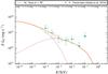 |
Fig. 7 Synchrotron and IC SEDs (thin lines, red) computed for the compression phase and the sum of the two contributions (thick line, orange) plotted together with the Fermi data of Cyg X-1 published in Zanin et al. (2016). In this case, we have adopted a strong magnetic field (χB = 0.5) and fixed the acceleration efficiency to ηNT = 0.01. The observing angle is φobs = 30°. |
The collective clump-jet interaction luminosity in the 0.1−100 GeV range, calculated averaging over one orbit5, and the computed clump evolution for a jet inclination with the line of sight of φobs = 30°, are ~ 1035 (ηNT/ 0.1) erg s-1 for Cyg X-1 and ~ 1036 (ηNT/ 0.1) erg s-1 for Cyg X-3, with an uncertainty of a factor of approximately 0.5–2 (including the high and the low B cases in that range). Assuming that the jet in Cyg X-1 is perpendicular to the orbital plane, its inclination with the line of sight is φobs ~ 30° (Orosz et al. 2011). In Cyg X-3, the jet inclination may be similar or even smaller (e.g., Mioduszewski et al. 2001; Dubus et al. 2010a; however Martí et al. 2001). Section 4 shows that DC values of approximately 1 are expected. Therefore, taking into account that the GeV luminosity in Cyg X-1 and Cyg X-3 are ~ 5 × 1033 (Zanin et al. 2016) and ~ 3 × 1036 erg s-1 (Fermi LAT Collaboration et al. 2009), respectively, one can derive the required non-thermal efficiency to be (ηNT/ 0.1) ≈ 0.05 for Cyg X-1, and ~ 3 for Cyg X-3 (for φobs = 30°; ~ 0.5 for φobs ~ 0°).
For Cyg X-1 the observational constraints only require a very modest non-thermal fraction ~ 1%. A comparison with Fermi data published in Zanin et al. (2016) is shown in Fig. 7, in which a rather strong magnetic field (χB = 0.5) and a fixed acceleration efficiency (ηNT = 0.01) were needed to reproduce the observational data, assuming DC = 1. We note that although this is a simplified model, it is interesting that it can approximately match the Fermi data.
A similar toy-application of our model to Cyg X-3 could be also performed (not shown here), for parameters similar to those of Cyg X-1 but with a much larger non-thermal fraction. However, in this case the energetics is rather demanding (~ 30%). Nevertheless, our calculations are obtained by fixing Γj = 2, while in fact different Γj-values are possible, and despite the relation between Γj and the Lorentz factor of the shocked jet flow being non-trivial (it depends on the postshock flow re-acceleration), slightly faster jets could alleviate the tight energetics for the Cyg X-3-like scenario. In addition, adopting a low magnetic field and the (probable) possibility of DC of a few would relax further the energetic constraints. Finally, the numerical calculations we carried out are also likely to underestimate the non-thermal emission because the computational grid encloses a relatively small region. Part of the radiation and the last stages of the clump evolution were not accounted for (see Sect. 3).
Values of DC ≪ 1 would lead to flares rather than to a smoother clump-jet interaction continuum. This requires a much higher degree of inhomogeneity than assumed in most of this work, because strong changes in Rc,min and Rc,max are not possible and DC is not very sensitive to α. However, as noted in Sect. 4, the radiation luminosity is proportional to χ− 1/2, meaning that for the same parameters, very inhomogeneous winds interacting with jets will be on average less radiatively efficient than moderately inhomogeneous ones.
The adiabatic index is constant in the code, although adopting  yields similar hydrodynamical results. The
  -value also quantitatively affects the non-thermal processes because they depend on the kinetic-to-internal energy conversion. However, we consider the related lack of precision acceptable given the numerous simplified assumptions adopted.
Acknowledgments
We thank the anonymous referee for the constructive and useful comments. We acknowledge support by the Spanish Ministerio de Economía y Competitividad (MINECO/FEDER, UE) under grants AYA2013-47447-C3-1-P and AYA2016-76012-C3-1-P with partial support by the European Regional Development Fund (ERDF/FEDER), MDM-2014-0369 of ICCUB (Unidad de Excelencia “María de Maeztu”), and the Catalan DEC grant 2014 SGR 86. This research has been supported by the Marie Curie Career Integration Grant 321520. V.B.-R. also acknowledges financial support from MINECO and European Social Funds through a Ramón y Cajal fellowship. This work is supported by ANPCyT (PICT 2012-00878). X.P.-F. also acknowledges financial support from Universitat de Barcelona and Generalitat de Catalunya under grants APIF and FI (2015FI_B1 00153), respectively. G.E.R. and S.dP. are supported by grant PIP 0338, CONICET. D.K. acknowledges financial support by a grant-in-aid for Scientific Research (KAKENHI, No. 24105007-1) from the Ministry of Education, Culture, Sports, Science and Technology of Japan (MEXT).
References
- Albert, J., Aliu, E., Anderhub, H., et al. 2007, ApJ, 665, L51 [NASA ADS] [CrossRef] [Google Scholar]
- Araudo, A. T., Bosch-Ramon, V., & Romero, G. E. 2009, A&A, 503, 673 [NASA ADS] [CrossRef] [EDP Sciences] [Google Scholar]
- Bednarek, W. 2013, Astropart. Phys., 43, 81 [NASA ADS] [CrossRef] [Google Scholar]
- Bodaghee, A., Tomsick, J. A., Pottschmidt, K., et al. 2013, ApJ, 775, 98 [NASA ADS] [CrossRef] [Google Scholar]
- Bordas, P., Yang, R., Kafexhiu, E., & Aharonian, F. 2015, ApJ, 807, L8 [NASA ADS] [CrossRef] [Google Scholar]
- Bosch-Ramon, V. 2012, A&A, 542, A125 [NASA ADS] [CrossRef] [EDP Sciences] [Google Scholar]
- Bosch-Ramon, V. 2013, A&A, 560, A32 [NASA ADS] [CrossRef] [EDP Sciences] [Google Scholar]
- Bosch-Ramon, V. 2015, A&A, 575, A109 [NASA ADS] [CrossRef] [EDP Sciences] [Google Scholar]
- Bosch-Ramon, V., & Barkov, M. V. 2016, A&A, 590, A119 [NASA ADS] [CrossRef] [EDP Sciences] [Google Scholar]
- Bosch-Ramon, V., & Khangulyan, D. 2009, Int. J. Mod. Phys. D, 18, 347 [NASA ADS] [CrossRef] [Google Scholar]
- Bosch-Ramon, V., Romero, G. E., & Paredes, J. M. 2006, A&A, 447, 263 [NASA ADS] [CrossRef] [EDP Sciences] [Google Scholar]
- Colella, P., & Woodward, P. R. 1984, J. Comput. Physics, 54, 174 [Google Scholar]
- de la Cita, V. M., Bosch-Ramon, V., Paredes-Fortuny, X., Khangulyan, D., & Perucho, M. 2016, A&A, 591, A15 [NASA ADS] [CrossRef] [EDP Sciences] [Google Scholar]
- Donat, R., & Marquina, A. 1996, J. Comput. Phys., 125, 42 [NASA ADS] [CrossRef] [Google Scholar]
- Donat, R., Font, J. A., Ibáñez, J. M. l., & Marquina, A. 1998, J. Comput. Phys., 146, 58 [NASA ADS] [CrossRef] [Google Scholar]
- Drury, L. O. 1983, Rept. Progr. Phys., 46, 973 [Google Scholar]
- Dubus, G. 2013, A&ARv, 21, 64 [NASA ADS] [CrossRef] [Google Scholar]
- Dubus, G., Cerutti, B., & Henri, G. 2010a, A&A, 516, A18 [NASA ADS] [CrossRef] [EDP Sciences] [Google Scholar]
- Dubus, G., Cerutti, B., & Henri, G. 2010b, MNRAS, 404, L55 [NASA ADS] [Google Scholar]
- Fermi LAT Collaboration, Abdo, A. A., Ackermann, M., et al. 2009, Science, 326, 1512 [NASA ADS] [CrossRef] [PubMed] [Google Scholar]
- Hamann, W.-R., Oskinova, L. M., & Feldmeier, A. 2008, in Clumping in Hot-Star Winds, Proc. Int. Workshop, 75 [Google Scholar]
- Liermann, A., Hamann, W.-R., Feldmeier, A., et al. 2010, Rev. Mex. Astron. Astrofis. Conf. Ser., 38, 50 [NASA ADS] [Google Scholar]
- Malyshev, D., Zdziarski, A. A., & Chernyakova, M. 2013, MNRAS, 434, 2380 [NASA ADS] [CrossRef] [Google Scholar]
- Martí, J. M., & Müller, E. 1996, J. Comput. Phys., 123, 1 [NASA ADS] [CrossRef] [Google Scholar]
- Martí, J., Paredes, J. M., & Peracaula, M. 2001, A&A, 375, 476 [NASA ADS] [CrossRef] [EDP Sciences] [Google Scholar]
- Mignone, A., Plewa, T., & Bodo, G. 2005, ApJS, 160, 199 [NASA ADS] [CrossRef] [Google Scholar]
- Mioduszewski, A. J., Rupen, M. P., Hjellming, R. M., Pooley, G. G., & Waltman, E. B. 2001, ApJ, 553, 766 [NASA ADS] [CrossRef] [Google Scholar]
- Miškovičová, I., Hell, N., Hanke, M., et al. 2016, A&A, 590, A114 [NASA ADS] [CrossRef] [EDP Sciences] [Google Scholar]
- Moffat, A. F. J. 2008, in Clumping in Hot-Star Winds, eds. W.-R. Hamann, A. Feldmeier, & L. M. Oskinova, Proc. Int. Workshop, 17 [Google Scholar]
- Moffat, A. F. J., & Corcoran, M. F. 2009, ApJ, 707, 693 [NASA ADS] [CrossRef] [Google Scholar]
- Muijres, L. E., de Koter, A., Vink, J. S., et al. 2011, A&A, 526, A32 [Google Scholar]
- Orosz, J. A., McClintock, J. E., Aufdenberg, J. P., et al. 2011, ApJ, 742, 84 [NASA ADS] [CrossRef] [Google Scholar]
- Owocki, S. P., & Cohen, D. H. 2006, ApJ, 648, 565 [NASA ADS] [CrossRef] [Google Scholar]
- Owocki, S. P., Romero, G. E., Townsend, R. H. D., & Araudo, A. T. 2009, ApJ, 696, 690 [NASA ADS] [CrossRef] [Google Scholar]
- Perucho, M., & Bosch-Ramon, V. 2008, A&A, 482, 917 [NASA ADS] [CrossRef] [EDP Sciences] [Google Scholar]
- Perucho, M., & Bosch-Ramon, V. 2012, A&A, 539, A57 [NASA ADS] [CrossRef] [EDP Sciences] [Google Scholar]
- Pittard, J. M. 2007, ApJ, 660, L141 [NASA ADS] [CrossRef] [Google Scholar]
- Puls, J., Vink, J. S., & Najarro, F. 2008, A&ARv, 16, 209 [NASA ADS] [CrossRef] [EDP Sciences] [Google Scholar]
- Rahoui, F., Lee, J. C., Heinz, S., et al. 2011, ApJ, 736, 63 [NASA ADS] [CrossRef] [Google Scholar]
- Romero, G. E., Torres, D. F., Kaufman Bernadó, M. M., & Mirabel, I. F. 2003, A&A, 410, L1 [NASA ADS] [CrossRef] [EDP Sciences] [Google Scholar]
- Romero, G. E., Del Valle, M. V., & Orellana, M. 2010, A&A, 518, A12 [NASA ADS] [CrossRef] [EDP Sciences] [Google Scholar]
- Runacres, M. C., & Owocki, S. P. 2002, A&A, 381, 1015 [NASA ADS] [CrossRef] [EDP Sciences] [Google Scholar]
- Sabatini, S., Tavani, M., Striani, E., et al. 2010, ApJ, 712, L10 [NASA ADS] [CrossRef] [Google Scholar]
- Szostek, A., & Zdziarski, A. A. 2008, MNRAS, 386, 593 [NASA ADS] [CrossRef] [Google Scholar]
- Tavani, M., Bulgarelli, A., Piano, G., et al. 2009, Nature, 462, 620 [NASA ADS] [CrossRef] [PubMed] [Google Scholar]
- Yoon, D., Zdziarski, A. A., & Heinz, S. 2016, MNRAS, 456, 3638 [NASA ADS] [CrossRef] [Google Scholar]
- Zanin, R., Fernández-Barral, A., de Oña Wilhelmi, E., et al. 2016, A&A, 596, A55 [NASA ADS] [CrossRef] [EDP Sciences] [Google Scholar]
- Zdziarski, A. A., Malyshev, D., Chernyakova, M., & Pooley, G. G. 2016a, MNRAS, submitted [arXiv:1607.05059] [Google Scholar]
- Zdziarski, A. A., Segreto, A., & Pooley, G. G. 2016b, MNRAS, 456, 775 [NASA ADS] [CrossRef] [Google Scholar]
All Tables
Values of the integrated emission in the 0.1–100 GeV band, given in erg s-1, considering an observer angle of φobs = 30°.
All Figures
|
Fig. 1 Density maps of the clump-jet interaction simulation that illustrate the clump evolution after ~ 73, 521, 596, 708, and 822 s (or, equivalently, to approximately 0.5, 3.5, 4.1, 4.8, and 5.6 in Rc/vsh units). |
| In the text | |
|
Fig. 2 Doppler boosting factor for φobs = 0°. The grey lines represent the computed streamlines, which are numbered. |
| In the text | |
|
Fig. 3 Compression-phase electron energy distribution for the individual streamlines (thin lines), and the total electron distribution (thick lines). Left panel: low magnetic field case (χB = 10-3). Right panel: high magnetic field case (χB = 1). |
| In the text | |
|
Fig. 4 Spectral energy distributions for the five stages shown in Fig. 1. Stage 1 corresponds to the compression phase, whereas stage 3 is the disruption phase; χB = 10-3 is adopted, and φobs = 30°. |
| In the text | |
|
Fig. 5 Top panel: synchrotron and IC SEDs for the compression phase φobs = 0, 30, and 90°, and χB = 10-3. The thin lines represent the emission without taking into account gamma-ray absorption due to electron-positron pair creation, i.e. the production SED. Middle panel: the same as for the top panel but for χB = 1. Bottom panel: a comparison between the SEDs of the compression and disruption phases. |
| In the text | |
|
Fig. 6 Top panel: duty-cycle in the radius ranges 1−2 R0, 2−3 R0, 1−3 R0, and > 3 R0 for a wind clump number distribution n ∝ Rc− α. A value α ~ 5 represents a wind dominated by small clumps, whereas α2 ~ 2.5 is an observational value for Wolf-Rayet (WR) stars; R0 is the minimum clump size given by Eq. (1). Bottom panel: duty-cycle weighted by the effective section of the shock, and therefore its potential luminosity, shown in units of the luminosity L0 produced in the interaction of one clump of R = R0 with the jet. The case > 3 R0 is not shown as it may imply jet disruption. |
| In the text | |
|
Fig. 7 Synchrotron and IC SEDs (thin lines, red) computed for the compression phase and the sum of the two contributions (thick line, orange) plotted together with the Fermi data of Cyg X-1 published in Zanin et al. (2016). In this case, we have adopted a strong magnetic field (χB = 0.5) and fixed the acceleration efficiency to ηNT = 0.01. The observing angle is φobs = 30°. |
| In the text | |
Current usage metrics show cumulative count of Article Views (full-text article views including HTML views, PDF and ePub downloads, according to the available data) and Abstracts Views on Vision4Press platform.
Data correspond to usage on the plateform after 2015. The current usage metrics is available 48-96 hours after online publication and is updated daily on week days.
Initial download of the metrics may take a while.