| Issue |
A&A
Volume 604, August 2017
|
|
|---|---|---|
| Article Number | A109 | |
| Number of page(s) | 18 | |
| Section | Cosmology (including clusters of galaxies) | |
| DOI | https://doi.org/10.1051/0004-6361/201629591 | |
| Published online | 22 August 2017 | |
Weak-lensing shear estimates with general adaptive moments, and studies of bias by pixellation, PSF distortions, and noise
Argelander-Institut für Astronomie, Universität Bonn, Auf dem Hügel 71, 53121 Bonn, Germany
e-mail: This email address is being protected from spambots. You need JavaScript enabled to view it.
Received: 26 August 2016
Accepted: 18 May 2017
Abstract
In weak gravitational lensing, weighted quadrupole moments of the brightness profile in galaxy images are a common way to estimate gravitational shear. We have employed general adaptive moments (GLAM ) to study causes of shear bias on a fundamental level and for a practical definition of an image ellipticity. The GLAM ellipticity has useful properties for any chosen weight profile: the weighted ellipticity is identical to that of isophotes of elliptical images, and in absence of noise and pixellation it is always an unbiased estimator of reduced shear. We show that moment-based techniques, adaptive or unweighted, are similar to a model-based approach in the sense that they can be seen as imperfect fit of an elliptical profile to the image. Due to residuals in the fit, moment-based estimates of ellipticities are prone to underfitting bias when inferred from observed images. The estimation is fundamentally limited mainly by pixellation which destroys information on the original, pre-seeing image. We give an optimised estimator for the pre-seeing GLAM ellipticity and quantify its bias for noise-free images. To deal with images where pixel noise is prominent, we consider a Bayesian approach to infer GLAM ellipticity where, similar to the noise-free case, the ellipticity posterior can be inconsistent with the true ellipticity if we do not properly account for our ignorance about fit residuals. This underfitting bias, quantified in the paper, does not vary with the overall noise level but changes with the pre-seeing brightness profile and the correlation or heterogeneity of pixel noise over the image. Furthermore, when inferring a constant ellipticity or, more relevantly, constant shear from a source sample with a distribution of intrinsic properties (sizes, centroid positions, intrinsic shapes), an additional, now noise-dependent bias arises towards low signal-to-noise if incorrect prior densities for the intrinsic properties are used. We discuss the origin of this prior bias. With regard to a fully-Bayesian lensing analysis, we point out that passing tests with source samples subject to constant shear may not be sufficient for an analysis of sources with varying shear.
Key words: gravitational lensing: weak / methods: data analysis / methods: statistical
© ESO, 2017
1. Introduction
Over the past decade measurements of distortions of galaxy images by the gravitational lensing effect have developed into an important, independent tool for cosmologists to study the large-scale distribution of matter in the Universe and its expansion history (recent reviews: Schneider 2006; Munshi et al. 2008; Hoekstra & Jain 2008; Massey et al. 2010; Kilbinger 2015). These studies exploit the magnification and shear of galaxy light bundles by the tidal gravitational field of intervening matter. The shear gives rise to a detectable coherent distortion pattern in the observed galaxy shapes. The distortions are usually weak, only of the order of a few per cent of the unlensed shape of a typical galaxy image. Therefore, the key to successfully devising gravitational shear as cosmological tool is accurate measurements of the shapes of many, mostly faint and hardly resolved galaxy images.
There has been a boost of interest in methods of shape measurements in anticipation of the gravitational lensing analysis of the upcoming next generation of wide-field imaging surveys (e.g. Euclid; Laureijs et al. 2011). Despite being sufficient for contemporary surveys, current methodologies are not quite at the required level of accuracy to fully do justice to the quantity of cosmological information we expect from future lensing surveys (Heymans et al. 2006; Massey et al. 2007). The challenge all methodologies face is that observable, noisy (post-seeing) galaxy images are modifications of the actual (pre-seeing) image owing to instrumental and possible atmospheric effects. Post-seeing galaxy images are subject to pixellation as well as instrumental noise, sky noise, photon noise, and random overlapping with very faint objects (Kitching et al. 2012; Hoekstra et al. 2015). In addition, galaxies are not intrinsically circular such that their ellipticities are noisy estimators of the cosmic distortion. Current theoretical work consequently focuses on sources of bias in shape measurements, such as pixel-noise bias, shape-noise bias, underfitting bias, colour gradients, or several selection biases (Hirata & Seljak 2003; Hirata et al. 2004; Mandelbaum et al. 2005; Melchior et al. 2010; Viola et al. 2011; Melchior & Viola 2012; Kacprzak et al. 2012; Massey et al. 2013; Semboloni et al. 2013).
One major source of bias is the pixel-noise bias or simply noise bias hereafter. This bias can at least partly be blamed on the usage of point estimates of galaxy shapes in a statistical analysis, that is single-value estimators of galaxy ellipticities (Refregier et al. 2012). This begs the question of whether it is feasible to eradicate noise bias by means of a more careful treatment of the statistical uncertainties in the measurement of galaxy ellipticities within a fully Bayesian framework. Indeed recent advances in image processing for weak gravitational lensing strongly support this idea, at least for the inference of constant shear (Sheldon 2014; Bernstein & Armstrong 2014, BA14 hereafter; Bernstein et al. 2016, BAKM16 hereafter). In contrast, the contemporary philosophy with point estimates is to perform elaborate, time-consuming calibrations of biased estimators by means of simulated images; the calibration accuracy is, additionally, only as good as the realism of simulated images (e.g. Hoekstra et al. 2015). It is the case that code implementations of non-Bayesian techniques are typically an order of magnitude or more faster than Bayesian codes which could be a decisive factor for upcoming surveys.
Here we take a new look into possible causes of bias in shear measurements on a fundamental level. To this end, we examine, step-by-step with increasing complexity, a fully-Bayesian lensing analysis based on weighted brightness moments of galaxy images (Gelman et al. 2013; MacKay 2003). While the method in BA14 and BAKM16 is set in Fourier space, we work with moments in angular space which has benefits in the case of correlated noise or missing pixels in realistic images. Moment-based methods as ours are non-parametric; this means they are free from assumptions about the galaxy brightness profile. They hence appear to be advantageous for reducing bias, but nonetheless the specific choice of the adaptive weight for the moments is known to produce bias (Viola et al. 2014; Voigt & Bridle 2010). The origin of this problem, which principally also affects unweighted moments, becomes obvious in our formalism. We define as practical measure of galaxy shape a generalization of the impractical ellipticity ϵ expressed in terms of unweighted moments (Kaiser et al. 1995; Seitz & Schneider 1997, SS97 hereafter). Being Bayesian, our measurement of ellipticity results in a Monte-Carlo sample of the probability distribution function (PDF) of ϵ which should be propagated in a fully Bayesian analysis. That is: we do not devise point estimators in order to ideally stay clear of noise bias. This overall approach of general adaptive moments (GLAM ) is inspired by and comparable to Bernstein & Jarvis (2002) apart from the Bayesian framework and some technical differences: (i) for any adaptive weight, the perfectly measured GLAM ellipticity is an unbiased estimator of gravitational shear unaffected by shape-noise bias; (ii) the adaptive weight may have a non-Gaussian radial profile; (iii) our inference of the pre-seeing ellipticity is realised as forward-fitting of elliptical profiles (so-called templates), that is we do not determine the brightness moments of the post-seeing image and correct them to estimate the pre-seeing moments (cf. Hirata & Seljak 2003; Mandelbaum et al. 2005).
As a disclaimer, the GLAM methodology outlined here is prone to bias, even where a fully Bayesian analysis can be realised, and, at this stage, its performance is behind that of other techniques. The aim of this paper is to elucidate causes of bias, instead of proposing a new technique that is competitive to existing techniques. However, these findings are also relevant for other methodologies because model-based or moment-based approaches are linked to GLAM .
For this paper, we exclude bias from practically relevant factors: the insufficient knowledge of the PSF or noise properties, blending of images, and the selection of source galaxies (see e.g. Heymans et al. 2006; Hartlap et al. 2011; Dawson et al. 2016). We focus on the core of the problem of shape measurements which is the inference of pre-seeing ellipticities from images whose full information on the brightness profile have been lost by instrumental limitations.
The paper is laid out as follows. In Sect. 2, we introduce the formalism of GLAM for a practical definition of ellipticity with convenient transformation properties under the action of gravitational shear. We also analytically investigate the limits of measuring the pre-seeing ellipticity from a noise-free but both PSF-convolved and pixellated image. In Sect. 3, we construct a statistical model for the GLAM ellipticity of noisy post-seeing images. We then study the impact of inconsistencies in the posterior model of ellipticity in three, increasingly complex scenarios. First, we analyse with independent exposures of the same pre-seeing image the ellipticity bias due to a misspecified likelihood in the posterior (underfitting bias). Second, we consider samples of noisy images with the same ellipticity but distributions of intrinsic properties such as sizes or centroid positions. Here a new contribution to the ellipticity bias emerges if the prior densities of intrinsic properties are incorrectly specified (prior bias). Third in Sect. 4, we perform numerical experiments with samples of noisy galaxy images of random intrinsic shapes that are subject to constant shear. With these samples we study the impact of inconsistent ellipticity posteriors on shear constraints (shear bias). We also outline details on our technique to Monte-Carlo sample ellipticity or shear posteriors. We discuss our results and possible improvements of the GLAM approach in Sect. 5.
2. General adaptive moments
2.1. Definition
Let I(x) be the light distribution in a galaxy image of infinite resolution and without noise where x is the position on the sky. A common way of defining a (complex) ellipticity of a galaxy image uses the quadrupole moments,  (1)of I(x) relative to a centroid position,
  (2)of the image (e.g. Bartelmann & Schneider 2001). For real applications, the quadrupole moments are soundly defined only if they involve a weight, decreasing with separation from the centroid position X0, because galaxies are not isolated so that the normalisation
  and the brightness moments diverge. Hirata & Seljak (2003, H03 hereafter) address the divergence problems by realising an adaptive weighting scheme by minimising the error functional, sometimes dubbed the energy functional,
 ![Mathematical equation: \begin{equation} \label{eq:functional} E(\vec{p}|I)= \frac{1}{2} \int\d^2x\; \Big[I(\vec{x})-Af(\rho)\Big]^2, \end{equation}](/articles/aa/full_html/2017/08/aa29591-16/aa29591-16-eq8.png) (3)with the quadratic form
(3)with the quadratic form  (4)and the second-order tensor
  (5)The tensor M is expressed in terms of the complex ellipticity e = e1 + ie2 and the size T of the image; f(ρ) is a weight function that HS03 chose to be a Gaussian weight f(ρ) = e− ρ/ 2. In comparison to HS03, we have slightly changed the definition of ρ for convenience: here we use ρ instead of ρ2. The set p = (A,x0,M), comprises a set of six parameters on which the functional E depends for a given galaxy image I.
Frequently another definition of complex ellipticity, the ϵ-ellipticity, is more convenient (sometimes also known as the third flattening). It arises if we write ρ in the form  (6)where V is symmetric. Obviously, we have V2 = M or
  . By writing V in the form
  (7)we see that V2 = M implies 2T = t2 (1 + | ϵ | 2), and
  (8)We henceforth use ϵ as parametrisation of M because ϵ is an unbiased estimator of reduced shear in the absence of a PSF and pixellation (SS97). Conversely, the ellipticity e has to be calibrated with the distribution of unsheared ellipticities which poses another possible source of bias in a lensing analysis (H03).
As generally derived in Appendix A, the parameters p at the minimum of (3) are:  (9)and
  (10)where
  is a constant. These equations are derived by HS03 for a Gaussian f(ρ), for which we have f′(ρ): = df/ dρ = − f/ 2. This shows that the best-fitting f(ρ) has the same centroid and, up to a scalar factor, the same second moment M = V2 as the with f′(ρ) adaptively weighted image I(x). This is basically also noted in Lewis (2009) where it is argued that the least-square fit of any sheared model to a pre-seeing image I(x) provides an unbiased estimate of the shear, even if it fits poorly.
In this system of equations, the centroid x0 and tensor M are implicitly defined because both f(ρ) and f′(ρ) on the right-hand-side are functions of the unknowns x0 and M: the weights adapt to the position, size, and shape of the image. Equations (9) and (10) therefore need to be solved iteratively. The iteration should be started at a point which is close to the final solution. Such a starting point could be obtained by using the image position, determined by the image detection software, as initial value for x0, and tensor M determined from a circular weight function with the same functional form as f. Nevertheless, there is no guarantee that the solution of this set of equations is unique. In fact, for images with two brightness peaks one might suspect that there are multiple local minima in p of the functional E. This may occur, for instance, in the case of blended images. One standard solution to this particular problem is to identify blends and to remove these images from the shear catalogue. Alternatively we could in principle try to fit two template profiles to the observed image, that is by adding a second profile E2(p2 | I) to the functional (3) and by minimising the new functional with respect to the parameter sets p and p2 of both profiles simultaneously.
2.2. Interpretation
If an image I(x) has confocal elliptical isophotes, with the same ellipticity for all isophotes, one can define the ellipticity of the image uniquely by the ellipticity of the isophotes. In this case, the ellipticity ϵ defined by the minimum of (3) coincides with the ellipticity of the isophotes for any weight f. We show this property in the following.
Assume that the brightness profile I(x) is constant on confocal ellipses so that we can write I(x) = S(ζ) where ζ: = (x − xc)TB-2(x − xc). Here xc denotes the centre of the image, and the matrix elements of B describe the size and the shape of the image, in the same way as we discussed for the matrix V before. The function S(ζ) describes the radial brightness profile of the image. We start by writing (9) in the form  (11)and introduce the transformed position vector z = B-1(x − xc), or x = Bz + xc. Then the previous equation becomes
  (12)where in terms of z the quadratic form ρ is
  (13)From these equations, we can see that x0 = xc is the solution of (12) since then ρ is an even function of z, S is an even function of z, whereas the term in the parenthesis of (12) is odd, and the integral vanishes due to symmetry reasons. Thus we found that our adaptive moments approach yields the correct centre of the image.
Next, we rewrite (10) in the form  (14)where β, see Eq. (10), is a constant factor (see Appendix A.3). We again used the transformation from x to z = B-1(x − xc) and employed the fact that x0 = xc. Accordingly, we have ρ = zTBV-2Bz. We now show that the solution of (14) is given by V = λB with λ being a scalar factor. Using this Ansatz, we get ρ = λ-2 | z | 2, and (14) can be written, after multiplying from the left and from the right by B-1, as
  (15)Since both S and f′ in the numerator depend solely on | z | 2, the tensor on the right hand side is proportional to the unit tensor 1, and (15) becomes a scalar equation for the scalar λ,
  (16)whose solution depends on the brightness profile S and the chosen weight function f. However, the fact that B differs from V only by the scalar factor λ implies that the derived ellipticity ϵ of V is the same as that of the elliptical image. Therefore we have shown that the approach of adapted moments recovers the true ellipticity with elliptical isophotes for any radial weight function f.
For a general brightness profile of the image, the interpretation of the GLAM ellipticity ϵ is less clear, and the ellipticity generally depends on the weight f. Nevertheless, ϵ is uniquely defined as long as a minimum of the functional (3) can be found. More importantly, for any weight f the GLAM ellipticity obeys the same simple transformation law under the action of gravitational shear, as shown in the following section.
2.3. Transformation under shear
We now consider the effect of a shear γ = γ1 + iγ2 and convergence κ on the GLAM ellipticity ϵ (Bartelmann & Schneider 2001). For an image with no noise, no pixellation, and no PSF convolution the ellipticity ϵ should be an unbiased estimate of the reduced shear g = g1 + ig2 = γ (1 − κ)-1. This is clearly true for sources that intrinsically have circular isophotes since the isophotes of the sheared images are confocal ellipses with an ellipticity ϵ = g. The minimum of (3) is hence at g by means of the preceding discussion.
For general images, let ϵs = ϵs,1 + iϵs,2 be the complex ellipticity of the image in the source plane and ϵ = ϵ1 + iϵ2 its complex ellipticity in the lens plane. We show now that for any brightness profile and template f(ρ), GLAM ellipticities have the extremely useful property to transform under the action of a reduced shear according to  (17)This is exactly the well-known transformation obtained from unweighted moments (SS97). To show this generally for GLAM , let Is(y) be the surface brightness of an image in the source plane with source plane coordinates y. The centroid y0 and moment tensor Ms of Is are defined by the minimum of (3) or, alternatively, by the analog of Eqs. (9) and (10) through
  (18)and
  (19)with
  (20)The ellipticity ϵs is given by
  (21)We now shear the image Is. The shear and the convergence are assumed to be constant over the extent of the image, that is lens plane positions x are linearly mapped onto source plane positions y by virtue of
  where
where  (22)xc and yc are such that the point xc is mapped onto the point yc by the lens equation, and both are chosen to be the central points around which the lens equation is linearised. We then find for the centroid y0 in the source plane
  (23)where
  . This then yields for (20)
  (24)In the next step, the expression (18) for the source centre can be rewritten by transforming to the image coordinates and using the conservation of surface brightness Is(y(x)) = I(x):
  (25)With the same transformation, we rewrite the moment tensor (19) as
  (26)On the other hand, minimising the functional (3) for the surface brightness I(x) in the lens plane yields the expressions (9) and (10) for x0 and M, respectively. We then see that Eqs. (25), (26) and (9), (10) agree with each other, if we set
  (27)for which ρs = ρ. In particular, this shows that the centre x0 of the image is mapped onto the centre y0 of the source.
The relation  (28)can be rewritten in terms of the square roots of the matrix M as
  (29)where
  is uniquely defined by requiring that for the symmetric, positive-definite matrix Ms, Vs is symmetric and positive-definite. Although both V and
  are symmetric,
  is in general not. Therefore Vs cannot be readily read off from (29). Instead, we use a rotation matrix
  (30)to write
 ![Mathematical equation: \begin{equation} \mat{V}_{\rm s}^2 = {\cal A}\mat{V}\mat{R}^{-1}(\varphi)\mat{R}(\varphi)\mat{V}{\cal A} = [\mat{R}(\varphi)\mat{V}{\cal A}]^{\rm T}[\mat{R}(\varphi)\mat{V}{\cal A}]. \end{equation}](/articles/aa/full_html/2017/08/aa29591-16/aa29591-16-eq102.png) (31)If we now choose ϕ to be such that
(31)If we now choose ϕ to be such that  is symmetric, then
  . After a bit of algebra, we find that the rotation angle ϕ is given through
  (32)and we obtain as final result Vs as in (21) with
  (33)The inverse of (33) is given by
  (34)We recover for the GLAM ellipticity ϵ exactly the transformation law of unweighted moments (SS97). The GLAM ellipticity ϵ is therefore an unbiased estimator of the reduced shear g along the line-of-sight of the galaxy, and there is no need to determine unweighted moments.
As a side remark, the transformation between ϵ and ϵs is a linear conformal mapping from the unit circle onto the unit circle, and from the origin of the ϵ-plane onto the point − g in the ϵs-plane. If | g | > 1, then g has to be replaced by 1 /g∗ in Eq. (34), but we shall not be concerned here with this situation in the strong lensing regime.
2.4. Point spread function and pixellation
We have defined the GLAM ellipticity ϵ of an image I(x) relative to an adaptive weight f(ρ). This definition is idealised in the sense that it assumes an infinite angular resolution and the absence of any atmospheric or instrumental distortion of the image. Equally important, it ignores pixel noise. In this section, we move one step further to discuss the recovery of the original ϵ of an image after it has been convolved with a PSF and pixellated. The problem of properly dealing with noise in the image is discussed subsequently.
Let Ipre(x) be the original image prior to a PSF convolution and pixellation. This we call the “pre-seeing” image. Likewise, by the vector Ipost of Npix values we denote the “post-seeing” image that has been subject to a convolution with a PSF and pixellation. For mathematical convenience, we further assume that Ipre(x) is binned on a fine auxiliary grid with N ≫ Npix pixels of solid angle Ω. We list these pixel values as vector Ipre. The approximation of Ipre(x) by the vector Ipre becomes arbitrarily accurate for N → ∞. Therefore we express the post-seeing image Ipost = LIpre by the linear transformation matrix L applied to the pre-seeing image Ipre. The matrix L with N × Npix elements combines the effect of a (linear) PSF convolution and pixellation. Similarly, we bin the template f(ρ) in the pre-seeing frame to the grid of Ipre, and we denote the binned template by the vector fρ; as usual, the quadratic form ρ is here a function of the variables (x0,ϵ,t), Eq. (6). The GLAM parameters ppre of the pre-seeing image are given by the minimum of E(p | Ipre), or approximately by  (35)For the recovery of the pre-seeing ellipticity ϵ, the practical challenge is to derive the pre-seeing parameters ppre from the observed image Ipost in the post-seeing frame. For this task, we assume that the transformation L is exactly known. We note that a linear mapping L is an approximation here; we ignore the nonlinear effects in the detector (Plazas et al. 2014; Gruen et al. 2015; Niemi et al. 2015; Melchior et al. 2015).
For a start, imagine a trivial case where no information is lost by going from Ipre to Ipost. We express this case by a transformation L that can be inverted, which means that N = Npix and L is regular. We then obtain ppre by minimising Epre(p | L-1Ipost) with respect to p: we map Ipost to the pre-seeing frame and analyse Ipre = L-1Ipost there. This is equivalent to minimising the form (Ipost − ALfρ)T(LLT)-1(Ipost − ALfρ) in the post-seeing frame.
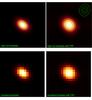 |
Fig. 1 Examples of GLAM templates in the pre-seeing frame, fρ (top left), and the post-seeing frame, Lfρ (other panels); the templates are Gaussian radial profiles with f(ρ) = e− ρ/ 2. The bottom left panel simulates only pixellation, whereas the right column also shows the impact of a PSF, indicated in the top right corner, without (top) and with pixellation (bottom). |
For realistic problems where L-1 does not exist, because N ≫ Npix, this trivial case at least suggests to determine the minimum ppost of the new functional  (36)as estimator of ppre. This way we are setting up an estimator by forward-fitting the template fρ to the image in the post-seeing frame with the matrix U being a metric for the goodness of the fit. Clearly, should L-1 exist we recover (35) only by adopting U = (LLT)-1. So we could equivalently obtain ppre, without bias, by fitting Lfρ to the observed image Ipost in this case. However, realistically L is singular: the recovery of ppre from (36) can only be done approximately. Then we could at least find an optimal metric to minimise the bias. We return to this point shortly. In any case, the metric has to be positive-definite and symmetric such that always Epost ≥ 0. We note that the moments at the minimum of (36) are related but not identical to the adaptive moments in the post-seeing frame. To obtain the latter we would fit a pixellated fρ with U = 1 to Ipost. The bottom and top right images in Fig. 1 display examples of post-seeing templates that are fitted to a post-seeing image to estimate ppre with the functional (36).
For singular L, the minimum of the functional yields an unbiased ppre for any U if
-
1.
Ipre(x) has confocal elliptical isophotes with the radial brightness profile S(x);
-
2.
and if we choose f(ρ) = S(ρ) as GLAM template;
-
3.
and if Epost has only one minimum (non-degenerate).
To explain, due to 1. and 2. we find a vanishing residual  (37)at the minimum of Epre and consequently Epre(ppre | Ipre) = 0. At the same time for any metric U, we also have Epost(ppre | Ipost) = 0 because Ipost − ALfρ = LRpre = 0 for p = ppre. Because of the lower bound Epost ≥ 0, these parameters ppre have to coincide with a minimum of Epost and hence indeed ppost = ppre. We note that the previous argument already holds for the weaker condition LRpre = 0 so that a mismatch between Ipre and the template at ppre produces no bias if the mapped residuals vanish in the post-seeeing frame. In addition, if this is the only minimum of Epost then the estimator ppost is also uniquely defined (condition 3). An extreme example of a violation of condition 3 is the degenerate case Npix = 1: the observed image consists of only one pixel. Then every parameter set (x0,ϵ,t) produces Epost = 0, if A is chosen correspondingly. But this should be a rare case because it is not expected to occur for Npix> 6, thus for images that span over more pixels than GLAM parameters.
A realistic pre-seeing image is neither elliptical nor is our chosen template f(ρ) likely to perfectly fit the radial light profile of the image, even if it were elliptical. This mismatch produces a bias in p only if L is singular, and the magnitude of the bias scales with the residual of the template fit in the pre-seeing frame. To see this, let  be the best-fitting template Afρ with parameters ppre. The residual of the template fit in the pre-seeing frame is
  . In the vicinity of ppre, we express the linear change of Afρ for small δp by its gradient at ppre,
  (38)where
  (39)Each column Gi of the matrix G denotes the change of Afρ with respect to pi. Therefore, close to ppre we find the Taylor expansion
  (40)Furthermore, since ppre is a local minimum of Epre, Eq. (35), we find at the minimum the necessary condition
  (41)This means that the residual Rres is orthogonal to every Gi. Now let
  be the residual mapped to the post-seeing frame. Then (36) in the vicinity to ppre is approximately
  (42)which we obtain by plugging (40) into (36). This approximation is good if the bias is small, by which we mean that the minimum ppost of Epost(p | Ipost) is close to ppre. As shown in Aitken (1934) in the context of minimum-variance estimators, the first-order bias δpmin = ppost − ppre that minimises (42) is then given by
  (43)with UL: = LTUL. This reiterates that the bias δpmin always vanishes either for vanishing residuals Rpre = 0, or if L-1 exists and we choose U = (LLT)-1 as metric. The latter follows from Eq. (43) with UL = 1 and Eq. (41). We note that δpmin does not change if we multiply U by a scalar λ ≠ 0. Thus any metric λU generates as much bias as U.
With regard to an optimal metric U, we conclude from Eq. (43) and GTRpre = 0 that we can minimise the bias by the choice of U for which UL ≈ 1, or if ∥ LTUL − 1 ∥ 2 is minimal with respect to the Frobenius norm ∥ Q ∥ 2 = tr(QQT). This optimised choice of U corresponds to the so-called pseudo-inverse (LLT)+ of LLT (Press et al. 1992). The pseudo-inverse is the normal inverse of LLT if the latter is regular.
A practical computation of U = (LLT)+ could be attained by choosing a set of orthonormal basis function bi in the pre-seeing frame, or approximately a finite number Nbase of basis functions that sufficiently describes images in the pre-seeing frame. For every basis function, one then computes the images Lbi and the matrix  (44)The pseudo-inverse of this matrix is the metric in the post-seeing frame.
Specifically, for images that are only pixellated the matrix LLT is diagonal. To see this, consider pixellations that map points ei in the pre-seeing frame to a single pixels e′(ei) in the post-seeing frame, or Lei = e′(ei); both ei and e′(ei) are unit vectors from the standard bases in the two frames. According to (44), the matrix LLT = ∑ ie′(ei) [ e′(ei) ] T is then always diagonal, typically proportional to the unit matrix, and easily inverted to obtain the optimal metric U. Unfortunately, this U only makes the linear-order bias (43) vanish while we still can have a higher-order bias because of the singular L.
2.5. Similarity between model-based and moment-based techniques
Through the formalism in the previous sections it becomes evident that there is no fundamental difference between model-based techniques and those involving adaptive moments. Model-based techniques perform fits of model profiles to the observed image, whereas moment-based ellipticities with the adaptive weight f′(ρ) are equivalently obtained from the image by fitting the ellipticial profile f(ρ) to the image. This requires, however, the existence of a unique minimum of the functional E(p | I) which we assume throughout the paper. We note that the similarity also extends to the special case of unweighted moments in Eqs. (1) and (2) which are in principle obtained by fitting f(ρ) = ρ since f′(ρ) = 1 in this case.
Nonetheless one crucial difference to a model-fitting technique is that a fit of f(ρ) does not assume a perfect match to I(x): the functional E(p | I) needs to have a minimum, but the fit is allowed to have residuals Rpre, this means E(p | I) ≠ 0 at the minimum. As shown, for the estimator based on (36) this may cause bias, Eq. (43), but only when analysing post-seeing images hence for L ≠ 1. In practice, different methodologies to estimate the pre-seeing moment-based ellipticity certainly use different approaches. Our choice of a forward-fitting estimator (36) is very specific but is optimal in the sense that it is always unbiased for LRpre = 0 or regular L. Yet other options are conceivable. For instance, we could estimate moments in the post-seeing frame first and try to map those to the pre-seeing frame (e.g. H03 or Melchior et al. 2011, which aim at unweighted moments). It is then unclear which weight is effectively applied in the pre-seeing frame. Therefore the expression Eq. (43) for the bias is strictly applicable only to our estimator and adaptive moments. But it seems plausible that the bias of estimators of pre-seeing moments generally depends on the residual Rpre since the brightness moments x0,i and Mij are the solutions to a best-fit of elliptical templates.
In the literature the problem of bias due to residuals in model fits is known as model bias or underfitting bias (Zuntz et al. 2013; Bernstein 2010). Consequently, moment-based techniques are as prone to underfitting bias as model-based methodologies.
3. Statistical inference of ellipticity
Realistic galaxy images I are superimposed by instrumental noise δI. Therefore the pre-seeing GLAM ellipticity can only be inferred statistically with uncertainties, and it is, according to the foregoing discussion, subject to underfitting bias. For a statistical model of the ellipticity ϵ, we exploit the previous conclusions according to which the ellipticity of I(x) for the adaptive weight f′(ρ) is equivalent to ϵ of the best-fitting template f(ρ). This renders the inference of ϵ a standard forward-fit of a model ALf(ρ) to I.
We consider post-seeing images I with Gaussian noise δI, that means images I = Ipost + δI. The covariance of the noise is N = ⟨ δIδIT ⟩, while Ipost = LIpre is the noise-free image in the post-seeing frame. A Gaussian noise model is a fair assumption for faint galaxies in the sky-limited regime (Miller et al. 2007). Possible sources of noise are: read-out noise, sky noise, photon noise, or faint objects that blend with the galaxy image. If an approximate Gaussian model is not applicable, the following model of the likelihood has to be modified accordingly.
The statistical model of noise are given by the likelihood ℒ(I | p) of an image I = LIpre + δI given the GLAM parameters p. We aim at a Bayesian analysis for which we additionally quantify our prior knowledge on parameters by the PDF Pp(p). We combine likelihood and prior to produce the marginal posterior  (45)of ellipticity by integrating out the nuisance parameters (x0,A,t); the constant normalisation of the posterior is irrelevant for this paper but we assume that the posterior is proper (it can be normalised). Our choice for the numerical experiments in this study is a uniform prior Pp(p) for positive sizes t and amplitudes A, ellipticities | ϵ | < 1, and centroid positions x0 inside the thumbnail image. As known from previous Bayesian approaches to shear analyses, the choice of the prior affects the consistency of the ellipticity posteriors (see, e.g. BA14). The origin of the prior-dependence will become clear in Sect. 3.3.
With regard to notation, we occasionally have to draw random numbers or vectors of random numbers x from a PDF P(x) or a conditional density P(x | y). We denote this by the shorthand x ~ P(x) and x ~ P(x | y), respectively. As common in statistical notation, distinct conditional probability functions may use the same symbol, as for instance the symbol P in P(x | y) and P(y | x).
3.1. Caveat of point estimates
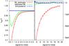 |
Fig. 2 Toy-model demonstration of a maximum-likelihood estimator (red), a maximum-likelihood estimator with first-order bias correction (green), and an estimator exploiting the full posterior (blue). Data points display the estimator average (y-axis) over 106 data points at varying signal-to-noise levels (x-axis). The true value to be estimated is x = 1. The panels show different signal-to-noise regimes; − nppt denotes y = 1 − n/ 103. |
The bias in a lensing analysis is not only affected by how we statistically infer galaxy shapes but also how we process the statistical information later on. To demonstrate in this context the disadvantage of point estimators in comparison to a fully Bayesian treatment, we consider here a simplistic nonlinear toy model. This model has one parameter x and one single observable y = x3 + n that is subject to noise n. By n ~ N(0,σ) we draw random noise from a Gaussian distribution N(0,σ) with mean zero and variance σ. From the data y, we statistically infer the original value of x. Towards this goal we consider the (log-)likelihood of y given x which is − 2lnℒ(y | x) = (y − x3)2σ-2 + const.
A maximum likelihood estimator of x is given by xest = y1 / 3, the maximum of ℒ(y | x). We determine the bias of xest as function of signal-to-noise ratio (S/N) x/σ by averaging the estimates of Nreal = 106 independent realisations of y. The averages and the standard errors are plotted as red line in Fig. 2. Clearly, xest is increasingly biased low towards lower S/N levels. In the context of lensing, this would be noise bias. As an improvement we then correct the bias by employing the first-order correction in Refregier et al. (2012) for each realisation of y. As seen in the figure, this correction indeed reduces the systematic error, but nevertheless breaks down for S/N ≲ 3.
On the other hand in a fully Bayesian analysis, we obtain constraints on x that are consistent with the true value for any S/N. For this purpose, we make Nreal independent identically distributed realisations (i.i.d.) yi and combine their posterior densities Ppost(x | yi) ∝ ℒ(yi | x) Pprior(x) by multiplying the likelihoods; we adopt a uniform (improper) prior Pprior(x) = const. This gives us for y = (y1,...,yNreal), up to a normalisation constant, the combined posterior  (46)As expected due to the asymptotic normality of posteriors (under regularity conditions), for i.i.d. experiments yi the product density is well approximated by a Gaussian N(x0,σx) and is consistent with the true value x (van der Vaart 1998). We plot values of x0 and σx in Fig. 2 as blue data points.
In conclusion, keeping the full statistical information Ppost(x | y) in the inference of x yields consistent constraints over the entire S/N range probed: the noise bias vanishes. Also note that the Bayesian approach has not substantially increased the error σx compared to the error of the point estimator (relative sizes of error bars); both approaches have similar efficiency.
3.2. Likelihood model and underfitting bias
Inspired by the foregoing Bayesian toy model that is free of noise bias, we set up a Bayesian approach for GLAM ellipticities. To construct a likelihood for a GLAM fit in the pre-seeing frame, we first consider, similar to Sect. 2.4, the trivial case where L is regular. This is straightforward since we can map the noisy image I → L-1I back to the pre-seeing frame and determine the noise residual for given pre-seeing p,  (47)The inverse noise covariance in the pre-seeing frame is LTN-1L. The logarithmic likelihood of δIpre(p) in the Gaussian case is thus
  (48)where “const.” expresses the normalisation of the likelihood. Therefore, we can equivalently write the pre-seeing fit in terms of available post-seeing quantities. We note here that the transform LRpre of the (unknown) pre-seeing residual is for singular L and Rpre ≠ 0 not equal to the post-seeing residual Rpost, which we defined in a least-square fit of ALfρ to Ipost (see Sect. 2.4).
In reality, L is singular so the previous steps cannot be applied. Nevertheless, Eq. (48) is the correctly specified likelihood of a forward fit if the model m(p): = Afρ + Rpre perfectly describes the brightness profile Ipre for some parameters ptrue. Therefore we expect no inconsistencies for singular L as long as the correct Rpre can be given. Since Rpre is unknown, however, we investigate in the following the impact of a misspecified likelihood that does not properly account for our ignorance in the pre-seeing residuals. We do this by assuming Rpre ≡ 0 and employing  (49)Obviously, this is a reasonable approximation of (48) if ∥ LRpre ∥ ≪ ∥ I ∥ so that residuals are only relevant if they are not small when compared to the image in the post-seeing frame. It also follows from Eq. (48) that for LRpre = 0 the likelihood is correctly specified even if Rpre ≠ 0 and L being singular, similar to the noise-free case. More generally we discuss later in Sect. 5 how we could modify the likelihood ℒ(I | p) to factor in our insufficient knowledge about Rpre. Until then the approximation (49) introduces underfitting bias into the likelihood model, making it inconsistent with the true ppre.
To show the inconsistency, we proceed as in the foregoing section on the toy model. We consider a series of n i.i.d. realisations Ii of the same image Ipost and combine their likelihoods ℒ(Ii | p) for a given p into the joint (product) likelihood  (50)and we work out its limit for n → ∞. The joint likelihood can be written as
  (51)Here we have made use of the properties of the trace of matrices, namely its linearity
  and that
  . For large n, we can employ the asymptotic expressions
  (52)to the following effect:
  (53)Thus the joint likelihood peaks for n → ∞ at the minimum ppost of ∥ Ipost − ALfρ ∥ N. This is equivalent to the location of the minimum of Epost(p | Ipost), Eq. (36), with metric U = N-1. Consequently, as in the noise-free case, we find an inconsistent likelihood if the residual Rpre is non-vanishing and if LTN-1L is not proportional to the unity matrix. We additionally expect a smaller bias δp = ppost − ppre for smaller levels of residuals1.
With regards to the noise dependence of underfitting bias, we find that δp does not change if we increase the overall level of noise in the image I. This can be seen by scaling the noise covariance N → λ N with a scalar λ. Any value λ> 0 results in the same minimum location for Epost(p | Ipost) so that δp is independent of λ: there is no noise bias.
Moreover, the bias δp of a misspecified likelihood seems to depend on our specific assumption of a Gaussian model for the likelihood. It can be argued on the basis of general theorems on consistency and asymptotic normality of posteriors, however, that for n → ∞ we obtain the same results for other likelihood models under certain regularity conditions (van der Vaart 1998; Appendix B in Gelman et al. 2013). The latter requires continuous likelihoods that are identifiable, hence ℒ(I | p1) ≠ ℒ(I | p2) for p1 ≠ p2, and that the true ptrue is not at the boundary of the domain of all parameters p. This is stricter than our previous assumptions for the Gaussian model where we needed only a unique global maximum of the likelihood ℒ(Ipost | p). It could therefore be that a unique maximum is not sufficient for non-Gaussian likelihoods.
3.3. Prior bias
The foregoing section discusses the consistency of the likelihood of a single image I. We can interpret the analysis also in a different way: if we actually had n independent exposures Ii of the same pre-seeing image, then combining the information in all exposures results in a posterior  that is consistent with ppost for a uniform prior Pp(p) = 1. As discussed in van der Vaart (1998), the more general Bernstein-von Mises theorem additionally shows that under regularity conditions the choice of the prior is even irrelevant provided it sets prior mass around ppost (Cromwell’s rule). This might suggest that for a correctly specified likelihood ℒ(Ii | p), a fully Bayesian approach for the consistent measurement of ϵ might be found that is independent of the specifics of the prior and has no noise bias in the sense of Sect. 3.2. This is wrong as shown in the following.
Namely, in contrast to the previous simplistic scenario, sources in a lensing survey have varying values of p: they are intrinsically different. For more realism, we therefore assume now i = 1...n pre-seeing images that, on the one hand, shall have different centroid positions x0,i, sizes ti, amplitudes Ai but, on the other hand, have identical ellipticities ϵ. Our goal in this experiment is to infer ϵ from independent image realisations Ii = Ipost,i + δIi by marginalising over the 4n nuisance parameters qi = (x0,i,ti,Ai). This experiment is similar to the standard test for shear measurements where a set of different pre-seeing images is considered whose realisations Ii are subject to the same amount of shear (e.g. Bridle et al. 2010). As a matter of fact, the inference of constant shear from an ensemble of images would just result in 2n additional nuisance parameters for the intrinsic shapes with essentially the same following calculations.
Let Pq(qi) be the prior for the four nuisance parameters qi of the ith image and Pϵ(ϵ) = 1 a uniform prior for ϵ. We combine the GLAM parameters in pi: = (qi,ϵ), and we assume that all images have the same prior density and that the noise covariance N applies to all images. The marginal posterior of ϵ is then the integral  (54)with
  being a normalization constant.
The product of the likelihood densities inside the integral is given by  (55)Here we have taken into account that the GLAM parameters partly differ, indicated by the additional index in Ai and fρ,i. This is different in Eq. (53) where we take the product of full likelihoods in p-space without marginalization. In the limit of n → ∞, we find in addition to the relations (52) that
  (56)because δIi is uncorrelated to ALfρ,i so that
  vanishes on average for many δIi. Therefore, for the asymptotic statistic we can replace all Ii by Ipost,i in Eq. (55) to obtain
  (57)and, as a result, for Eq. (54)
  (58)where Pϵ(ϵ | Ipost,i) is the marginal ellipticity posterior for the ith noise-free image.
The limit (58) has the interesting consequence that the consistency with ppost of the marginal posterior depends on the specific choice of the prior density Pq(qi). To show this, consider one particular case in which, for simplicity, all pre-seeing images are identical such that Ipost,i ≡ Ipost. Then, according to (58), the ellipticity posterior converges in distribution to [ Pϵ(ϵ | Ipost) ] n which for n → ∞ peaks at the global maximum of Pϵ(ϵ | Ipost). It is then easy to see that we can always change the position of this maximum by varying the prior density in Pϵ(ϵ | Ipost). In particular, even if the likelihoods are correctly specified, we generally find an inconsistent marginal posterior depending on the prior. A similar argument can be made if Ipost,i ≠ Ipost,j for i ≠ j.
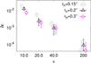 |
Fig. 3 Prior bias in the marginal posterior Pϵ(ϵ | I1,...,In) as function of S/N ν for different galaxy sizes rh (in arcsec). The posterior assumes a uniform prior. Shown is the error δϵ = | ϵ − ϵtrue | of the inferred ϵ for a true ϵtrue = 0.3 as obtained by combining the marginal posteriors of 5 × 10³ exposures of the same galaxy with random centroid positions. The pixel size 0.1 arcsec equals the PSF size (Moffat). Galaxy profiles and GLAM templates have a Sérsic profile with n = 2: there is no underfitting. |
For a concrete example, we perform for Fig. 3 a simulated analysis of 5 × 10³ noisy images with ϵtrue = 0.3. All pre-seeing images are identical to one particular template Afρ (Sérsic profile with n = 2). Therefore we have a correctly specified likelihood model and no underfitting. We adopt a uniform prior Pq(q) (and Pϵ(ϵ)). The details on the simulated images and their analysis are given in Sect. 4. For each data point, we plot the mean and variance of the marginal posterior Pϵ(ϵ | I1,...,In) relative to the true ellipticity ϵtrue as function of S/N ν and for different image sizes rh. Evidently, the bias δϵ increases for smaller ν thereby producing a noise-dependent bias which is not present when analysing the consistency of ℒ(I | p) of individual images as in Sect. 3.2.
The sensitivity of the posterior to the prior implies that consistency (for a correctly specified likelihood) could be regained by choosing an appropriate prior density Pq(qi). On the other hand, the dependence on the prior runs against the conventional wisdom that the prior should become asymptotically irrelevant for n → ∞ as the joint likelihood starts dominating the information on inferred parameters. Indeed, general theorems show this under certain regularity conditions (see e.g. discussion in Chap. 4 of Gelman et al. 2013). These conditions are, however, not given here because the total number of model parameters is not fixed but rather increases linearly with n due to a new set of nuisance parameters qi for every new galaxy image Ii. The observed breakdown of consistency is the result. A trivial (but practically useless) prior to fix the problem is one that puts all prior mass at the true values of the nuisance parameters which essentially leaves only ϵ as free model parameter. Likewise, an analysis with sources that knowingly have the same values for the nuisance parameters also yields consistent constraints; this is exactly what is done in Sect. 3.2. A non-trivial solution, as reported by BA14, is to use “correct priors” for the nuisance parameters that are equal to the actual distribution of q in the sample. On the downside, this raises the practical problem of obtaining correct priors from observational data.
In summary, for an incorrect prior of q, such as our uniform prior, we find a noise-dependent bias in the inferred ellipticity despite a fully Bayesian approach and a correctly specified likelihood. We henceforth call this bias “prior bias”. This emphasises the difference to the noise bias found in the context of point estimators.
4. Simulated shear bias
We have classified two possible sources of bias in our Bayesian implementation of adaptive moments: underfitting bias and prior bias. In this section, we study their impact on the inference of reduced shear g by using samples of mock images with varying S/N, galaxy sizes, and galaxy brightness profiles. In contrast to our previous experiments, the images in each sample have random intrinsic shapes but are all subject to the same amount of shear, and we perform numerical experiments to quantify the bias. Moreover, this section outlines practical details of a sampling technique for the posteriors of GLAM ellipticities and the reduced-shear, which is of interest for future applications (Sects. 4.4 and 4.5).
The PSF shall be exactly known for these experiments. For a large shear bias, we choose a relatively small PSF size and galaxy images that are not much larger than a few pixels. According to the discussion in Sect. 2.4, underfitting bias is mainly a result of pixellation which mathematically cannot be inverted. We note that a larger PSF size would reduce the underfitting bias since it spreads out images over more image pixels. Overall the values for shear bias presented here are larger than what is typically found in realistic surveys (e.g. Zuntz et al. 2013). We start this section with a summary of our simulation specifications.
4.1. Point-spread function
If not stated otherwise, our simulated postage stamps consist of 20 × 20 pixels (squares), of which one pixel has a size of 0.1′′; the simulated galaxies are relatively small with a half-light radius rh of only a few times the pixel size (0.15′′ ≤ rh ≤ 0.3′′). Additionally, we adopt an isotropic Moffat PSF, 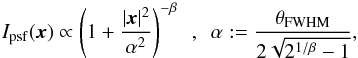 (59)with the full width half maximum (FWHM) of θFWHM = 0.1′′ and β = 5 (Moffat 1969).
4.2. GLAM template profiles
As GLAM templates we employ truncated Sérsic-like profiles with index n, ![Mathematical equation: \begin{equation} \label{eq:sersic} f(\rho)= \exp{\left(-\left[\frac{\rho}{\rho_0}\right]^{\frac{1}{2n}}\right)}\, h(\!\sqrt{\rho})~;~ h(x):=\frac{1}{\e^{5(x-3)}+1} \end{equation}](/articles/aa/full_html/2017/08/aa29591-16/aa29591-16-eq332.png) (60)and
(60)and  (61)(Capaccioli 1989). To avoid a numerical bias due to aliasing at the edges of the grid during the Fourier transformation steps in the sampling code, we have introduced the auxiliary function h(x) that smoothly cuts off the Sérsic profile beyond ρ ≈ 9. If f(ρ) were the radial light profile of an elliptical galaxy, the truncation would be located at about three half-light radii.
We use template profiles with n = 2 throughout. This index n falls between the values of n used for the model galaxies and thus is a good compromise to minimise the fit residual and thereby the underfitting bias.
4.3. Mock galaxy images
We generate postage stamps of mock galaxy images with varying half-light radii rh, radial light profiles, and signal-to-noise ratios ν. To this end, we utilise the code that computes the post-seeing GLAM templates (Appendix B). We consider pre-seeing images of galaxies with elliptical isophotes of three kinds of light profiles, Eq. (60): (1) exponential profiles with Sérsic index n = 1 (EXP; exponential), (2) de-Vaucouleur profiles with n = 4 (DEV; bulge-like) and (3) galaxies with profiles n = 2 that match the profile of the GLAM template (TMP; template-like). TMP galaxies hence cannot produce underfitting bias.
We devise uncorrelated Gaussian noise in the simulation of postage stamps. To determine the RMS variance σrms of the pixel noise for a given ν, let fi be the flux inside image pixels that is free of noise and ftot = ∑ ifi the total flux. From this, we compute a half-light flux threshold fth defined such that the integrated flux fhl = ∑ fi ≥ fthfi above the threshold is fhl = ftot/ 2 or as close as possible to this value. The pixels i with fi ≥ fth are defined to be within the half-light radius of the image; their number is Nhl: = ∑ fi ≥ fth; the integrated noise variance within the half-light radius is  . The signal-to-noise ratio within the half-light radius is therefore
  , or
, or  (62)Figure 4 depicts four examples with added noise for different ν.
 |
Fig. 4 Examples of simulated images of galaxies with random ellipticities. Signal-to-noise ratios from left to right and top to bottom: ν = 10, 20, 40, and 200. The radial light profile of the pre-seeing images is exponential with rh = 0.2′′; the pixel size is 0.1′′. The FWHM of the PSF is indicated by the circle in the top right corners. |
To simulate galaxy images with intrinsic ellipticities that are sheared by g, we make a random realisation of an intrinsic ellipticity ϵs and compute the pre-seeing ellipticity with (17). As PDF for the intrinsic ellipticities we assume a bivariate Gaussian with a variance of σϵ = 0.3 for each ellipticity component; we truncate the PDF beyond | ϵs | ≥ 1.
In realistic applications, centroid positions of galaxy images are random within an image pixel, so we average all our following results for bias over subpixel offsets within the quadratic solid angle of one pixel at the centre of the image. This means: in an sample of mock images, every image has a different subpixel position which is chosen randomly from a uniform distribution. In this averaging process, care has to be taken to perform an even sampling of subpixel offsets. To ensure this with a finite number of random points in all our following tests, we employ a subrandom Sobol sequence in two dimensions for the random centroid offsets (Press et al. 1992).
4.4. Monte-Carlo sampling of ellipticity posterior
For practical applications of a Bayesian GLAM analysis, we produce a Monte Carlo sample of the posterior Pϵ(ϵ | I), Eq. (45) with the approximate likelihood ℒ(I | p) in Eq. (49). This sample consists of a set (ϵi,wi) of 1 ≤ i ≤ Nreal pairs of values ϵi and wi, which determine the sampling position ϵi and a sampling weight wi. For this paper, we use Nreal = 50 sampling points. In contrast to a lensing analysis with single-valued point estimators of ellipticity, a Bayesian analysis employs the sample (ϵi,wi) of each galaxy. To attain the sample (ϵi,wi) we invoke the importance sampling technique (e.g. Marshall 1956; Kilbinger et al. 2010).
For this technique, we define an approximation Q(p) of Pp(p | I), the so-called importance distribution function, from which we draw a random sample pi. The ellipticity component ϵi of pi is then assigned the weight wi = Pp(pi | I) Q(pi)-1 which we normalise to ∑ iwi = 1 afterwards. As importance function, we use a multivariate Gaussian with mean at the maximum pml of the likelihood ℒ(I | p) and a covariance defined by the inverse Fisher matrix F-1 at the maximum (Fisher 1935; Tegmark et al. 1997). More implementation details are given in Appendix B.
If Q(p) is too different from Pp(p | I), the sample will be dominated by few points with large weights, usually due to sampling points in the tail of the posterior for which the importance function predicts a too low probability, this means wi becomes large. This is indicated by a small effective number  of points compared to Nreal. This can produce a poor convergence and thus extreme outliers in the analysis that merely appear to have tight constrains on ϵ. Typically affected by this are images that are both small compared to the pixel size and low in signal-to-noise. These images tend to exhibit posteriors that allow parameter solutions with small sizes t compared to the true t or high eccentricities | ϵ | ≳ 0.7, giving the posterior a complex, distinctly non-Gaussian shape. In future applications, this problem can be addressed by finding a better model of the importance function.
For the scope of this paper, we address this problem at the expense of computation time by increasing the number of sampling points and by resampling. This means: for Monte-Carlo samples with Neff<Nreal/ 2, we draw more samples from the importance distribution until Neff ≥ Nreal/ 2 in the expanded sample. By an additional rule, we stop this process if the expanded sample size becomes too large and reaches 10 × Nreal. This case is indicative of a failure of the importance sampling. If this happens, we switch to a time-consuming standard Metropolis algorithm to sample the posterior with 103 points after 102 preliminary burn-in steps (Metropolis et al. 1953). This technique does not assume a particular shape for the posterior but performs a random walk through the p space, thereby producing a correlated sample along a Monte-Carlo Markov chain. As symmetric proposal distribution for this algorithm, we adopt a multivariate Gaussian with covariance 1.5 × F-1; all points of the chain have equal weight wi; the starting point of the chain is pml. Finally, in the resampling phase, we bootstrap the expanded or Metropolis sample by randomly drawing Nreal points from it with probability wi (with replacement). All selected data points are given the equal weights  in the final catalogue.
4.5. Posterior density of reduced shear
For the inference of g, we convert the ellipticity posterior Pϵ(ϵ | I) into a posterior Pg(g | I) of shear. To this end, let us first determine the Pg(g | ϵ) for an exactly known ϵ. We express our uncertainty on the intrinsic ellipticity ϵs by the prior Ps(ϵs), and Pg(g) is our a-priori information on g. The values of g and ϵs shall be statistically independent, by which we mean that Psg(ϵs,g) = Ps(ϵs) Pg(g)2. Applying a marginalization over ϵs and then Bayes’ rule, we find  (63)or, equivalently,
  By
By  we denote the normalisation of Pg(g | ϵ),
  (66)The normalisation only depends on the modulus of ϵ for isotropic priors for symmetry reasons. The integration over the Dirac delta function δD(x) uses Eq. (17). The determinant | d2ϵs/ d2ϵ |, the Jacobian of the linear conformal mapping ϵs(g,ϵ), is a function of ϵ and g. For the weak lensing regime | g | ≤ 1 of interest, this is
  (67)(Geiger & Schneider 1998). To now account for the measurement error of ϵ in the shear posterior, we marginalise Pg(g | ϵ), Eq. (65), over ϵ with Pϵ(ϵ | I) as error distribution,
  (68)In our Monte Carlo scheme, we sample the ellipticity posterior of every galaxy i through (ϵij,wij) ~ Pϵ(ϵ | Ii) by 1 ≤ j ≤ Nreal values ϵij of ellipticity and statistical weight wij. To convert this sample to an approximation of the g posterior, we replace Pϵ(ϵ | Ii) inside the integral (68) by the point distribution ΣjwijδD(ϵ − ϵij),
  (69)For the following, we adopt a uniform prior for g, which means Pg(g) ∝ H(1 − | g |). For reasons discussed in Sect. 3.3, the prior on the nuisance ϵs presumably has to be equal to the distribution of intrinsic shapes for a consistent shear posterior. To investigate the sensitivity of shear bias as to Ps(ϵs) we therefore use two types of priors: the correct prior, which is the true intrinsic-shape distribution in Sect. 4.3, or a uniform prior H(1 − | ϵs |). For each prior Ps(ϵs), we numerically compute for different ϵ once and interpolate between them later on in (69). We finally combine the posteriors Pg(g | Ii) of all images Ii in the sample by multiplying posterior values on a g-grid. For this, we apply (69) to every galaxy in the sample independently.
4.6. Results
 |
Fig. 5 Plots of the multiplicative bias m for simulated images, based on Eq. (69), for two different priors Ps(ϵs) (filled data points: correct prior; open data points: uniform prior). Different styles for the data points indicate different image sizes rh, see key inside figure, while colours vary with galaxy type: GLAM template (TMP; red); exponential (EXP; green); bulge-like (DEV; blue). Data points for rh = 0.3′′, same galaxy type, and same prior are connected by dotted lines to guide the eye. The prior for galaxy sizes t, amplitudes A, and centroids x0 is uniform giving rise to noise-dependent prior bias; the constant offset of EXP and DEV is due to underfitting. A square image pixel has the size 0.1′′, which also equals the PSF size. Results for m for a larger PSF size can be found in Table 1. |
For each experiment, we consider a sample of statistically independent galaxy images  that are subject to the same reduced shear g but have random intrinsic ellipticities ϵs. To infer g from
  in a fully Bayesian manner, we compute the posteriors Pg(g | Ii) of g for every image Ii separately with Eq. (69) and then combine all posteriors by the product
  (70)This test is related, but not identical, to the ring test in Nakajima & Bernstein (2007): we do not fix the ellipticity magnitude | ϵs | during one test run but instead use a random sample of intrinsic ellipticities. Each galaxy sample consists of n = 5 × 10⁴ simulated noisy galaxy images to typically attain a precision for g of the order 10-3. This number applies for the non-uniform prior Ps(ϵs). The precision is lower for the less informative uniform prior. Moreover, for each galaxy with intrinsic ϵs we also use − ϵs in another image belonging to the sample. By doing so the mean of intrinsic ellipticities in an sample is always zero, which substantially reduces the numerical noise in the result. For every set of image parameters, we vary the input shear between the three values gtrue ∈ { 0, ± 0.05, ± 0.1 }. For these five measurements, let ⟨ g | gtrue ⟩ be the mean of the posterior (70) for a given gtrue of the sample. We then determine the multiplicative bias m and the additive bias c in
 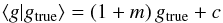 (71)by best-fitting m and c to the mean and dispersion of (70) for the three input values of gtrue; m shall be a real-valued number.
In Fig. 5, we plot m (filled data points) juxtaposed with the corresponding values based on a uniform prior (open data points); same data points indicate the same size rh while colours, varying by row, indicate the light profiles of the images. For the numbers in the table and the data points in the figure, error bars quantify a 68% posterior interval of the measurement around the quoted mean. The size of error bars account for pixel noise and shape noise. For the range of ν studied here, the impact of pixel noise is subdominant: the errors increase only between 10% and 20% from ν = 200 to ν = 10; the increase is larger for small images. Values for the additive bias c (not shown) for all profiles are small within a few 10-4, except at ν = 10 for DEV with rh = 0.15′′,0.2′′ and for TMP at 0.15′′: there c can reach negative amplitudes of the order of 10-3. This indicates that an additive bias could be relevant for image sizes close to the pixel size.
Multiplicative bias m in per cent for three profiles TMP, EXP, DEV, and sizes rh = 0.2′′ only.
In contrast, a multiplicative bias m is typically significant. At high S/N ν = 200, this bias in Fig. 5 is mainly underfitting bias which is consequently absent for TMP galaxies since their likelihood is correctly specified. The shear of bulge-like galaxies DEV, with steeper slope compared to f(ρ), is underestimated by m = − 9.6 ± 0.5%; the shear of exponential galaxies EXP, which have a shallower slope, is overestimated by m = + 7.7 ± 0.5%. These numbers are the mean and standard error for all galaxy sizes at ν = 200; they depend on the specific PSF and pixel sizes chosen for this experiment.
Compared to the underfitting bias at ν = 200, the bias m significantly drops if ν ≲ 20 for all galaxies, most prominently at rh = 0.15′′, but stays roughly constant within a couple of per cent otherwise. We attribute the noise-dependence of m to prior bias owing to our choice of an (incorrect) uniform prior for the nuisance parameters q of the images (see Sect. 3.3). The prior bias thus becomes only relevant here at sufficiently low S/N. The particular value of S/N is specific to the PSF size. This can be seen in Table 1 which lists estimates for m for galaxies, in a slightly smaller sample n = 2 × 10⁴, with size rh = 0.2′′ but for a modified, roughly twice as large PSF size 0.22′′. Now the noise-dependence of prior bias is already visible below ν ≲ 40. On the other hand, the underfitting bias, to be read off at high S/N ν = 200, is roughly halved since the images are spread out over more pixels.
The choice of a uniform prior for the intrinsic ellipticities, distinctively different from the true distribution of ϵs in the sample, has a negligible effect on shear bias here for both PSF sizes. Values of m between the two priors Ps(ϵs) are consistent, as found by comparing filled and open data points of same colour and at same ν in Fig. 5. Nevertheless, the resulting statistical errors of shear, as opposed to its bias, are larger by roughly the factor 1.7 with the uniform prior, which reflects the larger a-priori uncertainty on ϵs. This implies that a shear bias due to an incorrect prior Ps(ϵs) is negligible in this experiment.
5. Discussion
Unlike galaxy ellipticities defined in terms of unweighted moments, GLAM provide a practical definition of ellipticity with useful properties for any chosen adaptive weight f′(ρ): they (i) are identical with the ellipticity of isophotes of elliptical galaxy images; (ii) under the influence of shear they behave exactly like ϵ defined with unweighted moments; (iii) they are unbiased estimators of reduced shear; (i)−(iii) assume ideal conditions without pixellation, PSF convolution, or pixel noise. These effects fundamentally limit our ability to determine the GLAM ellipticity (see below). Under ideal conditions, see SS97, it is known that ϵ for unweighted moments already obeys (iii). However, unweighted moments are formally infinite for realistic galaxy images because of pixel noise so that weighting is a necessity which is done adaptively for GLAM . For adaptive weights, we have shown (i) and (ii) in Sects. 2.2 and 2.3. Their relevance as unbiased estimators for reduced shear, statement (iii), follows thereafter from (ii) and the conclusions in SS97 for unweighted moments. We emphasise that GLAM do not require “deweighting” in a lensing analysis (Melchior et al. 2011): the ellipticity in term of the weighted moments is actually unbiased. In particular, we do not have to devise the same weight function for all galaxies as any weight function equally obeys (ii). If the minimum of the functional (3) uniquely exists, the moments (x0,α MI) of the best-fitting template f(ρ) will, for a constant scalar α, be the adaptively weighted moments (x0,MI) of the galaxy light profile I(x) for the weight f′(ρ) (Appendix A). This means that the radial profile of the weight at separation r from the centroid is w(r) ∝ r-1dfr(r) / dr for a template profile fr(r): = f(r2). We exploited this relation between adaptive moments and moments of a best-fitting elliptical profile to analyse limits to adaptive moment-based methods under the loss of image information.
Namely, for realistic images subject to pixellation and PSF effects, underfitting bias can be present for GLAM if estimated from the post-seeing image. It potentially arises because of a loss of information on the pre-seeing galaxy image, fundamentally due to pixellation. To explore the limitations, we assume noise-free images and express in Sect. 2.4 the mapping between a pre-seeing and post-seeing image by the linear operation L. The pre-seeing adaptive moments are equivalent to a least-square fit with residual Rpre of an elliptical profile f(ρ) to the pre-seeing image I(x). If estimated from the post-seeing image whilst ignoring residuals, the inferred ellipticity is biased for LRpre ≠ 0and a singular L. The latter indicates a loss of information on the pre-seeing image. For noise-free images and the estimator (36) the bias is, to linear order, given by Eq. (43). In (36) the bias is optimally reduced through the metric U = (LLT)+. With this metric the estimator is unbiased for regular L, hence in principle also for an invertible convolution with an anisotropic PSF; invertible convolutions have kernels K(x) with  in the Fourier domain. Practically, however, a singular mapping is always present due to pixellation so that the quadratic estimator (36) could never fully remove underfitting bias.
The inference of GLAM ellipticity from noisy images with a likelihood that ignores fitting residuals produces underfitting bias; the underfitting bias depends on the correlation of pixel noise and its homogeneity over the image. To deal with pixel noise in images, we have put GLAM in a Bayesian setting in Sect. 3 by employing an approximate model (49) for the likelihood that ignores fit residuals and thus equals an imperfect model fit with an elliptical profile. We use this to explore the impact of a misspecified likelihood that, as a result, can be shown to be subject to underfitting bias. The bias is revealed in the limit of combining the likelihoods of n → ∞ independent exposures of the same image (see Sect. 3.2). To lowest order in Rpre, we find the bias to vanish if LTN-1L is proportional to the unit matrix. The underfitting bias is unchanged for a rescaled noise covariance: there hence is no noise bias from a misspecified likelihood. Additionally, the magnitude of bias depends on the details of N and can also emerge for L = 1 if N is not proportional to the unit matrix, which is the case for heterogeneous or correlated noise. Due to the close relation of GLAM ellipticity to other definitions of ellipticity we expect similar dependencies of bias on the noise covariance there, which may impact future calibration strategies in lensing applications because they apparently should not ignore cases of correlated or heterogeneous noise. We note that several steps in the reduction of lensing data can produce correlated pixel noise.
The underfitting bias from the likelihood can presumably be addressed at the expense of an increased statistical error, such as by means of a follow-up high-resolution survey that gathers statistical information on the residuals Rpre. First of all, one obvious way to reduce underfitting bias is to choose a template that provides a good fit to galaxy images to reduce the residuals. The optimal template has the profile fr(r) ∝ Sr(r) for a pre-seeing galaxy profile Sr(r); this also optimises the signal-to-noise ratio of the ellipticity (Bernstein & Jarvis 2002). Even so, realistic galaxies can never be perfectly fit by an elliptical model; there are always fitting residuals Rpre. To deal with these residuals, we can imagine a more elaborate Bayesian scheme where Rpre are additional nuisance parameters that we marginalise over by using an empirical distribution P(Rpre | p) of Rpre given p (prior), that is  (72)where ℒ(I | p,Rpre) is the likelihood of a post-seeing image, correctly specified by the post-seeing model m(p) = L(Afρ + Rpre) and the noise distribution. The marginalization would then increase the statistical uncertainty in the posterior Pϵ(ϵ | I) in Eq. (45). It is conceivable to measure the prior in a dedicated survey by assessing the distribution of residuals in template fits to high resolution, high S/N images. This approach would be similar to that of BA14 where a (correct) prior on galaxy-specific descriptors is needed. In comparison to BA14, it is noteworthy here that the residuals Rpre in the pre-seeing frame are those of sheared images for which we infer ϵ; no assumptions on the unsheared, source-plane images have to be made for this prior. All this, however, still has to be tested, and it is not clear how this can be properly implemented and if this marginalization is not the source of another bias.
A consistent likelihood of single images is not sufficient for a lensing analysis as new inconsistencies for ϵ or g can arise in samples of intrinsically different sources through incorrect priors for intrinsic source parameters, such as sizes or centroid positions (prior bias). Take for example our TMP galaxies in Sect. 4 which have a correctly specified likelihood by definition; they are free of underfitting bias. For the two experiments presented in Figs. 3 and 5, the source sample consists of pre-seeing images with an unknown distribution of intrinsic parameters. The first experiment considers samples with constant ellipticity, the second samples with constant reduced shear. Despite the absent underfitting, noise bias now emerges in both cases if we apply our uniform prior for the nuisance parameters in the marginal posterior of either ellipticity or reduced shear; see TMP data points at ν ≲ 20. We argue in Sect. 3.3 that the emerging noise bias is related to the specific choice of priors and can only be avoided by a special family of correct priors related to the maximum of the posterior of noise-free images. According to previous work, correct priors are the distributions of nuisance parameters of the sources in the sample which have to be defined externally (e.g. BA14, Miller et al. 2013; Kitching et al. 2008). A conceivable alternative to external priors, potentially worthwhile investigating in future studies, might be to specify the priors down to a family of distributions, so-called hyperpriors, with a finite, preferably small number of hyperparameters (Gelman et al. 2013). A hierarchical approach would then jointly determine the posterior density of ϵ or g and the hyperparameters from all Ii alone in a fully Bayesian way. Marginalising over the hyperparameters accounts for the uncertainty in the priors. We note that the incorrect uniform prior for ϵs in Fig. 5 has no significant impact on the shear bias (compare open to filled data points). Clearly, the importance of a correct prior depends on the type of nuisance parameter.
That prior bias in Fig. 5 or Table 1 becomes relevant only at low S/N can be understood qualitatively. For a sufficiently high S/N, the mass of an (identifiable) likelihood ℒ(Ipost | p) concentrates around ppost such that the prior Pp(p) details have no strong impact on the marginal posterior of one source. We also expect for high S/N the likelihood to be well approximated by a normal Gaussian with maximum ppost such that the marginalization over q = (A,t,x0) approximately yields a Gaussian posterior Pϵ(ϵ | Ipost) with maximum near ϵpost, which is the true pre-seeing ellipticity for a correctly specified likelihood. We note that the marginalization over q of a multivariate Gaussian with maximum at p0 = (ϵ0,q0) produces another Gaussian density with maximum at ϵ0. In addition, should the likelihood be misspecified, ϵpost will be prone to underfitting bias which is clearly visible by the offsets in m for EXP and DEV in Fig. 5.
Finally, we point out that while marginal posteriors Pϵ(ϵ | Ii), obtained on an image-by-image basis, are sufficient to infer a constant ellipticity (or shear) it is not obvious how to incoorporate them into a fully Bayesian analysis of sources with varying shear. For example, in a fully Bayesian inference of ellipticity correlations  for images ij at separation ϑ, we would compute the likelihood
  for given values of ξϑ and a range of ϑ, which principally requires the repeated shape measurements for the entire sample of images for every new ξϑ. This poses a practical, computational problem. Proposed solutions to this problem leave the path of a fully Bayesian analysis and commonly use unbiased point estimators of ϵi on a image-by-image basis as input for a statistical analysis (e.g. Miller et al. 2013). This technique has essentially been applied to all lensing analyses so far, but requires a calibration of the ellipticity estimates, especially for the noise bias. The recently proposed hierarchical Bayesian technique by Alsing et al. (2016), applied to data in Alsing et al. (2017), is closest to a fully Bayesian analysis in the above sense but also uses as input unbiased estimators of source ellipticities with a multivariate Gaussian probability density for the statistical errors of the estimates. Yet, it is surely conceivable to extend this technique by directly modelling the likelihood of source images Ii. To reverse-propagate our Pϵ(ϵ | Ii) to a posterior of ξϑ, we might be tempted here to Monte-Carlo a posterior PDF of ξϑ by independently drawing ellipticities ϵim ~ Pϵ(ϵ | Ii) from the marginal posteriors to produce realisations of a joint vector ϵm = (ϵ1m,...,ϵnm), which could be used with an estimator of ξϑ. Unfortunately, this falsely assumes a separable joint posterior
  with statistically independent ellipticities, potentially biasing (low) constraints on ξϑ. As alternative we speculate about the following hierarchical Bayesian scheme. We assume a parametric model
  for the joint posterior density of ellipticities that is determined by (i) the measured marginal ellipticities Pϵ(ϵ | Ii) and (ii) a set of unknown hyperparameters θ = (θ1,θ2,...) that quantify the correlations between the source ellipticities. A convenient choice in this respect seem to be copula models that are specified exactly that way (e.g. Sect. 2 in Takeuchi 2010). We further express our ignorance about θi by a (sufficiently uninformative) hyperprior Pθ(θ). We then produce realisations ϵm by first randomly drawing θm ~ Pθ(θ) followed by
  . A sample { ϵ1,ϵ2,... } of joint ellipticities is then utilised to propagate uncertainties on source ellipticities and their mutual correlations through the lensing analysis, based on an estimator for ξϑ given a joint sample ϵ. We note that in the limit ν → ∞ the hyperprior for θ becomes irrelevant because all marginal posteriors Pϵ(ϵ | Ii) will be sharply peaked at the true ellipticity (if correctly specified).
Incidentally, the bias δp in the likelihood and the underfitting bias in the noise-free case are equal for N-1 ∝ (LLT)+, which for regular L is equivalent to homogeneous, uncorrelated noise in the pre-seeing frame, which means we have LTN-1L ∝ 1.
This assumption would be false if shear and intrinsic ellipticity were correlated, for instance due to selection effects related to the shape of a sheared image (Hirata & Seljak 2003; Heymans et al. 2006). Thus correlations between intrinsic shapes and shear may affect Bayesian methodologies already at this level.
Acknowledgments
The authors are particularly grateful to Gary Bernstein who read and commented on an earlier manuscript of this paper. The comments lead to a substantial improvement. We would also like to thank Tim Schrabback for helpful discussions and comments, and our colleague Reiko Nakajima for organising a weekly seminar on shape measurements in our institute that triggered the research presented in this paper. We also acknowledge the comments by the referee of this paper that helped to clarify and revise certain points, in particular the section on the prior bias. This work has been supported by the Deutsche Forschungsgemeinschaft in the framework of the Collaborative Research Center TR33 “The Dark Universe”. Patrick Simon also acknowledges support from the German Federal Ministry for Economic Affairs and Energy (BMWi) provided via DLR under project No. 50QE1103.
References
- Aitken, A. 1934, On least squares and linear combination of observations, 55, 42 [Google Scholar]
- Alsing, J., Heavens, A., Jaffe, A. H., et al. 2016, MNRAS, 455, 4452 [NASA ADS] [CrossRef] [Google Scholar]
- Alsing, J., Heavens, A., & Jaffe, A. H. 2017, MNRAS, 466, 3272 [NASA ADS] [CrossRef] [Google Scholar]
- Bartelmann, M., & Schneider, P. 2001, Phys. Rep., 340, 291 [NASA ADS] [CrossRef] [Google Scholar]
- Bernstein, G. M. 2010, MNRAS, 406, 2793 [NASA ADS] [CrossRef] [Google Scholar]
- Bernstein, G. M., & Armstrong, R. 2014, MNRAS, 438, 1880 [NASA ADS] [CrossRef] [Google Scholar]
- Bernstein, G. M., & Jarvis, M. 2002, AJ, 123, 583 [NASA ADS] [CrossRef] [Google Scholar]
- Bernstein, G. M., Armstrong, R., Krawiec, C., & March, M. C. 2016, MNRAS, 459, 4467 [NASA ADS] [CrossRef] [Google Scholar]
- Bertin, E., & Arnouts, S. 1996, A&AS, 117, 393 [NASA ADS] [CrossRef] [EDP Sciences] [Google Scholar]
- Bezdek, J., Hathaway, R., Howard, R., Wilson, C., & Windham, M. 1987, J. Optim. Theory Appl., 54, 471 [CrossRef] [Google Scholar]
- Bridle, S., Balan, S. T., Bethge, M., et al. 2010, MNRAS, 405, 2044 [NASA ADS] [Google Scholar]
- Capaccioli, M. 1989, in World of Galaxies, eds. H. G. Corwin, Jr., & L. Bottinelli, 208 [Google Scholar]
- Dawson, W. A., Schneider, M. D., Tyson, J. A., & Jee, M. J. 2016, ApJ, 816, 11 [NASA ADS] [CrossRef] [Google Scholar]
- Fisher, R. A. 1935, J. Roy. Stat. Soc., 98, 39 [CrossRef] [Google Scholar]
- Frigo, M., & Johnson, S. G. 2005, Proc. IEEE, special issue on Program Generation, Optimization, and Platform Adaptation, 93, 216 [Google Scholar]
- Geiger, B., & Schneider, P. 1998, MNRAS, 295, 497 [NASA ADS] [CrossRef] [Google Scholar]
- Gelman, A., Carlin, J., Stern, H., et al. 2013, Bayesian Data Analysis, third edn., Chapman & Hall/CRC Texts in Statistical Science (Taylor & Francis) [Google Scholar]
- Gruen, D., Bernstein, G. M., Jarvis, M., et al. 2015, Journal of Instrumentation, 10, C05032 [CrossRef] [Google Scholar]
- Hartlap, J., Hilbert, S., Schneider, P., & Hildebrandt, H. 2011, A&A, 528, A51 [NASA ADS] [CrossRef] [EDP Sciences] [Google Scholar]
- Heymans, C., Van Waerbeke, L., Bacon, D., et al. 2006, MNRAS, 368, 1323 [NASA ADS] [CrossRef] [Google Scholar]
- Hirata, C., & Seljak, U. 2003, MNRAS, 343, 459 [NASA ADS] [CrossRef] [Google Scholar]
- Hirata, C. M., Mandelbaum, R., Seljak, U., et al. 2004, MNRAS, 353, 529 [NASA ADS] [CrossRef] [Google Scholar]
- Hoekstra, H., & Jain, B. 2008, Ann. Rev. Nucl. Part. Sci., 58, 99 [Google Scholar]
- Hoekstra, H., Herbonnet, R., Muzzin, A., et al. 2015, MNRAS, 449, 685 [NASA ADS] [CrossRef] [Google Scholar]
- Kacprzak, T., Zuntz, J., Rowe, B., et al. 2012, MNRAS, 427, 2711 [NASA ADS] [CrossRef] [Google Scholar]
- Kaiser, N., Squires, G., & Broadhurst, T. 1995, ApJ, 449, 460 [NASA ADS] [CrossRef] [Google Scholar]
- Kilbinger, M. 2015, Rep. Prog. Phys., 78, 086901 [Google Scholar]
- Kilbinger, M., Wraith, D., Robert, C. P., et al. 2010, MNRAS, 405, 2381 [NASA ADS] [Google Scholar]
- Kitching, T. D., Miller, L., Heymans, C. E., van Waerbeke, L., & Heavens, A. F. 2008, MNRAS, 390, 149 [NASA ADS] [CrossRef] [Google Scholar]
- Kitching, T. D., Balan, S. T., Bridle, S., et al. 2012, MNRAS, 423, 3163 [NASA ADS] [CrossRef] [Google Scholar]
- Laureijs, R., Amiaux, J., Arduini, S., et al. 2011, ArXiv e-prints [arXiv:1110.3193] [Google Scholar]
- Lewis, A. 2009, MNRAS, 398, 471 [NASA ADS] [CrossRef] [Google Scholar]
- MacKay, J. D. 2003, Information Theory, Inference, and Learning Algorithms (Cambridge, UK: Cambridge University Press) [Google Scholar]
- Mandelbaum, R., Hirata, C. M., Seljak, U., et al. 2005, MNRAS, 361, 1287 [NASA ADS] [CrossRef] [Google Scholar]
- Marquardt, D. 1963, J. Soc. Ind. Appl. Mathem., 11, 431 [Google Scholar]
- Marshall, A. 1956, in Symp. on Monte Carlo methods (Wiley), ed. M. Meyer, 123 [Google Scholar]
- Massey, R., Heymans, C., Bergé, J., et al. 2007, MNRAS, 376, 13 [NASA ADS] [CrossRef] [Google Scholar]
- Massey, R., Kitching, T., & Richard, J. 2010, Rep. Prog. Phys., 73, 086901 [Google Scholar]
- Massey, R., Hoekstra, H., Kitching, T., et al. 2013, MNRAS, 429, 661 [Google Scholar]
- Melchior, P., & Viola, M. 2012, MNRAS, 424, 2757 [NASA ADS] [CrossRef] [Google Scholar]
- Melchior, P., Böhnert, A., Lombardi, M., & Bartelmann, M. 2010, A&A, 510, A75 [NASA ADS] [CrossRef] [EDP Sciences] [Google Scholar]
- Melchior, P., Viola, M., Schäfer, B. M., & Bartelmann, M. 2011, MNRAS, 412, 1552 [NASA ADS] [CrossRef] [Google Scholar]
- Melchior, P., Suchyta, E., Huff, E., et al. 2015, MNRAS, 449, 2219 [NASA ADS] [CrossRef] [Google Scholar]
- Metropolis, N., Rosenbluth, A. W., Rosenbluth, M. N., Teller, A. H., & Teller, E. 1953, J. Chem. Phys., 21, 1087 [NASA ADS] [CrossRef] [Google Scholar]
- Miller, L., Kitching, T. D., Heymans, C., Heavens, A. F., & van Waerbeke, L. 2007, MNRAS, 382, 315 [NASA ADS] [CrossRef] [Google Scholar]
- Miller, L., Heymans, C., Kitching, T. D., et al. 2013, MNRAS, 429, 2858 [Google Scholar]
- Moffat, A. F. J. 1969, A&A, 3, 455 [NASA ADS] [Google Scholar]
- Munshi, D., Valageas, P., van Waerbeke, L., & Heavens, A. 2008, Phys. Rep., 462, 67 [NASA ADS] [CrossRef] [Google Scholar]
- Nakajima, R., & Bernstein, G. 2007, AJ, 133, 1763 [NASA ADS] [CrossRef] [Google Scholar]
- Niemi, S.-M., Cropper, M., Szafraniec, M., & Kitching, T. 2015, Exp. Astron., 39, 207 [NASA ADS] [CrossRef] [Google Scholar]
- Plazas, A. A., Bernstein, G. M., & Sheldon, E. S. 2014, Journal of Instrumentation, 9, C4001 [CrossRef] [Google Scholar]
- Press, W. H., Teukolsky, S. A., Vetterling, W. T., & Flannery, B. P. 1992, Numerical recipes in C. The art of scientific computing 2nd edn (Cambridge University Press) [Google Scholar]
- Refregier, A., Kacprzak, T., Amara, A., Bridle, S., & Rowe, B. 2012, MNRAS, 425, 1951 [NASA ADS] [CrossRef] [Google Scholar]
- Schneider, P. 2006, in Saas-Fee Advanced Course 33: Gravitational Lensing: Strong, Weak and Micro, eds. G. Meylan, P. Jetzer, P. North, P. Schneider, C. S. Kochanek, & J. Wambsganss, 269 [Google Scholar]
- Seitz, C., & Schneider, P. 1997, A&A, 318, 687 [NASA ADS] [Google Scholar]
- Semboloni, E., Hoekstra, H., Huang, Z., et al. 2013, MNRAS, 432, 2385 [NASA ADS] [CrossRef] [Google Scholar]
- Sheldon, E. S. 2014, MNRAS, 444, L25 [NASA ADS] [CrossRef] [Google Scholar]
- Takeuchi, T. T. 2010, MNRAS, 406, 1830 [NASA ADS] [Google Scholar]
- Tegmark, M., Taylor, A. N., & Heavens, A. F. 1997, ApJ, 480, 22 [NASA ADS] [CrossRef] [Google Scholar]
- van der Vaart, A. W. 1998, Asymptotic statistics, Cambridge Series in Statistical and Probabilistic Mathematics (Cambridge University Press) [Google Scholar]
- Viola, M., Melchior, P., & Bartelmann, M. 2011, MNRAS, 410, 2156 [NASA ADS] [CrossRef] [Google Scholar]
- Viola, M., Kitching, T. D., & Joachimi, B. 2014, MNRAS, 439, 1909 [NASA ADS] [CrossRef] [Google Scholar]
- Voigt, L. M., & Bridle, S. L. 2010, MNRAS, 404, 458 [NASA ADS] [Google Scholar]
- Zuntz, J., Kacprzak, T., Voigt, L., et al. 2013, MNRAS, 434, 1604 [NASA ADS] [CrossRef] [Google Scholar]
Appendix A: Least-square conditions
In this section, we derive general characteristics of GLAM parameters p = (A,x0,M) at a local minimum of the error functional E(p | I), Eq. (3). For convenience, we introduce the bi-linear scalar product  (A.1)to write the functional as
  (A.2)Notice that ρ: = (x − x0)TM-1(x − x0) is a function of p. The scalar product has the properties
  of which we make heavily use in the following.
Starting from here, we find as necessary condition for the least-square solution of any parameter pi: ![Mathematical equation: \appendix \setcounter{section}{1} \begin{eqnarray} \lefteqn{\frac{\partial E(\vec{p}|I)}{\partial p_i}=0}\\ &&\nonumber =\Ave{-\frac{\partial[Af(\rho)]}{\partial p_i},I(\vec{x})-Af(\rho)}+ \Ave{I(\vec{x})-Af(\rho),-\frac{\partial[Af(\rho)]}{\partial p_i}}\\ &&\nonumber =-2\Ave{\frac{\partial[Af(\rho)]}{\partial p_i},I(\vec{x})-Af(\rho)}\\ &&\nonumber =-2\Ave{\frac{\partial[Af(\rho)]}{\partial p_i},I(\vec{x})}+ 2A\Ave{\frac{\partial[Af(\rho)]}{\partial p_i},f(\rho)}, \end{eqnarray}](/articles/aa/full_html/2017/08/aa29591-16/aa29591-16-eq484.png) (A.3)or simply
(A.3)or simply ![Mathematical equation: \appendix \setcounter{section}{1} \begin{equation} \label{eq:mlcondition} \Ave{\frac{\partial[Af(\rho)]}{\partial p_i},A^{-1}I(\vec{x})}= \Ave{\frac{\partial[Af(\rho)]}{\partial p_i},f(\rho)} \end{equation}](/articles/aa/full_html/2017/08/aa29591-16/aa29591-16-eq485.png) (A.4)that is fulfilled for all pi.
(A.4)that is fulfilled for all pi.
Appendix A.1: Template normalisation
From (A.4) follows for the normalisation pi = A at the minimum of E(p | I) that  (A.5)
(A.5)
Appendix A.2: Image centroid position
For the least-square centroid position x0,i with i = 1,2 at the minimum of E(p | I), we find ∂ [ Af(ρ) ] /∂x0,i = Af′(ρ) ∂ρ/∂x0,i using f′(ρ): = df(ρ) / dρ. This can be expanded further by considering ![Mathematical equation: \appendix \setcounter{section}{1} \begin{eqnarray} \label{eq:rhox0} \frac{\partial\rho}{\partial x_{0,i}}&=& \frac{\partial}{\partial x_{0,i}} \sum_{k,l} (x_k-x_{0,k})[\mat{M}^{-1}]_{kl}(x_l-x_{0,l})\\ \nonumber &=& -\sum_{k,l} \left( \delta^{\rm K}_{ki}[\mat{M}^{-1}]_{il}(x_l-x_{0,l})+ \delta^{\rm K}_{li}[\mat{M}^{-1}]_{ki}(x_k-x_{0,k}) \right)\\ \nonumber &=& -2\sum_k[\mat{M}^{-1}]_{ki}(x_k-x_{0,k}) =-2\left[\mat{M}^{-1}(\vec{x}-\vec{x}_0)\right]_i. \end{eqnarray}](/articles/aa/full_html/2017/08/aa29591-16/aa29591-16-eq491.png) (A.6)Here we have exploited the symmetry [ M-1 ] ij = [ M-1 ] ji and introduced the Kronecker symbol
(A.6)Here we have exploited the symmetry [ M-1 ] ij = [ M-1 ] ji and introduced the Kronecker symbol  . Therefore we find for the ith component of the centroid position
 ![Mathematical equation: \appendix \setcounter{section}{1} \begin{equation} \Ave{Af^\prime(\rho)[\mat{M}^{-1}(\vec{x}-\vec{x}_0)]_i,f(\rho)-A^{-1}I(\vec{x})}=0 \end{equation}](/articles/aa/full_html/2017/08/aa29591-16/aa29591-16-eq494.png) (A.7)or, equally, for both centroid components combined
(A.7)or, equally, for both centroid components combined  (A.8)The scalar product on the left-hand-side has to vanish due to symmetry reasons. Therefore using the right-hand-side, we find at the minimum
  (A.9)This shows that the centroid x0 at the least-square point is the first-order moment x of the image I(x) weighted with the kernel f′(ρ). The weight is thus the derivative f′(ρ) not f(ρ).
Appendix A.3: Image second-order moments
For the components of M, we consider the least-square values of the inverse Wij = [ M-1 ] ij, hence values Wij for which ∂ [ Af(ρ) ] /∂Wij = Af′(ρ) ∂ρ/∂Wij vanishes. The function ρ can be expressed as  (A.10)using X: = (x − x0)(x − x0)T = XT and the relation tr(ABC) = tr(BCA) for traces of matrices. From this follows that ∂ρ/∂Wij = [ X ] ij = Xij, or
  (A.11)by employing Eq. (A.4). This set of (four) equations can compactly be written as
  (A.12)or utilising Eq. (A.5):
  (A.13)This last relation shows that the best-fitting template f(ρ) has, up to a constant scalar α, the same central second-order moments MI as the image,
  In particular, the best-fitting template Af(ρ) has, for a given profile f(s), the same ellipticity ϵ as the image I(x). Moreover, we derive from (A.13) the relation
  (A.17)The scalar prefactor equals β = − 2 for f(ρ) = e− ρ/ 2. We note that we have on the right-hand-side f(ρ) in the denominator rather than f′(ρ).
We evolve the expression of β a bit further by changing the variables Δx = M1 / 2y and hence  for ρ = ΔxTM-1Δx in the integrals of the denominator and nominator of β,
  (A.18)or after another change of variables
  and
and  ,
,  (A.19)where the last step assumes that the profile f(s) vanishes for s → ∞.
Appendix B: Importance sampling of posterior distribution

An overview of our algorithm for sampling the posterior Pp(p | I) is given by Algorithm 1, more details follow below.
For the importance sampling of the posterior GLAM variables p, we initially construct an analytical approximation Q(p) of the (full) posterior Pp(p | I): = ℒ(I | p) Pp(p) in Eq. (45), the so-called importance function. Our importance function is a local Gaussian approximation of ℒ(I | p) that is truncated for | ϵ | ≥ 1; Q(p) is hence defined by its mean and its covariance. As previously discussed, we ignore residuals and set Rpre ≡ 0 in Eq. (48) for the following.
For the mean pml of the Gaussian Q(p), we numerically determine the maximum-likelihood (ML) point of ℒ(I | p) by minimising (48) with respect to p. This is the most time consuming step in our algorithm, which is done in the following three steps.
-
1.
We quickly guess a starting point p0 of the centroid position x0 and the galaxy size t by measuring the unweighted first and second-order moments of the post-seeing postage stamp. The initial ellipticity ϵ is set to zero. Herein we ignore the PSF. Alternatively, one could use estimates from object detection software such as SExtractor if available (Bertin & Arnouts 1996).
-
2.
For an improved initial guess of the size t and the centroid position x0, starting from p0 we perform a series of one-dimensional (1D) searches wherein we vary one parameter pi while all other parameters pj with i ≠ j are fixed (coordinate descent; Bezdek et al. 1987). For each 1D search, we compute − 2lnℒ(I | p) at five points over the range of values of pi that are allowed according to the prior Pp(p). We spline interpolate between the points to estimate the global minimum
 . Then we update pi to the value and move on to the 1D search of the next parameter. After every update we replace A by its most likely value
 ![Mathematical equation: \appendix \setcounter{section}{2} \begin{equation} A_{\rm ml}= \frac{\vec{I}^{\rm T}\mat{N}^{-1}\mat{L}\vec{f}_\rho} {[\mat{L}\vec{f}_\rho]^{\rm T}\mat{N}^{-1}\mat{L}\vec{f}_\rho} \end{equation}](/articles/aa/full_html/2017/08/aa29591-16/aa29591-16-eq527.png) (B.1)(Eq. A.5) given the current values of (x0,ϵ,t). We carry out the searches first for the size t and then for the two components of the centroid position x0.
(B.1)(Eq. A.5) given the current values of (x0,ϵ,t). We carry out the searches first for the size t and then for the two components of the centroid position x0. -
3.
Starting from p in step 2, we apply the Levenberg-Marquardt algorithm (LMA) to iteratively approach pml (Marquardt 1963). This algorithm devises a linear approximation of Lfρ at p based on the partial derivatives of Lfρ. Our implementation of the LMA searches only in the directions of (x0,ϵ,t) and again updates A to Aml after each iteration as in step 2. We find a slow convergence for large ellipticities, that is | ϵ | ≳ 0.3. This is improved, however, by adding an extra 1D search for the size t, ϵ1 and ϵ2 after each LMA iteration with an interval width of ± 0.1t (10 spline points) and ± 0.1 (5 points) around the latest values of t and ϵi, respectively. For | ϵn | ≥ 0.6, we use 10 instead of 5 spline points which increases the accuracy for very elliptical objects. We repeat the LMA until iteration n> 5 for which | ϵn − 1 − ϵn | ≤ 10-4; we change this threshold to 2 × 10⁻⁵ once | ϵn | ≥ 0.6. The latter is needed because the change of ϵn at each iteration becomes small for high ϵ.
For the covariance of Q(p), we then numerically compute the elements Fij of the (expected) Fisher matrix F around the ML point pml, ![Mathematical equation: \appendix \setcounter{section}{2} \begin{equation} \label{eq:fisher} F_{ij}= \left( \frac{\partial[A\mat{L}\vec{f}_\rho]} {\partial p_i} \right)^{\rm T} \times\mat{N}^{-1} \times \left( \frac{\partial[A\mat{L}\vec{f}_\rho]} {\partial p_j} \right), \end{equation}](/articles/aa/full_html/2017/08/aa29591-16/aa29591-16-eq541.png) (B.2)by considering partial derivatives of the best-fitting GLAM templates (e.g. Tegmark et al. 1997). This gives us
(B.2)by considering partial derivatives of the best-fitting GLAM templates (e.g. Tegmark et al. 1997). This gives us ![Mathematical equation: \appendix \setcounter{section}{2} \begin{equation} Q(\vec{p})\propto \exp{\left( -\frac{1}{2} \left[\vec{p}-\vec{p}_{\rm ml}\right]^{\rm T} \mat{F} \left[\vec{p}-\vec{p}_{\rm ml}\right] \right)}\, H\left(P_{\rm p}(\vec{p})\right), \end{equation}](/articles/aa/full_html/2017/08/aa29591-16/aa29591-16-eq542.png) (B.3)where H(x) denotes the Heaviside step function. To quickly construct the Fisher matrix, we employ the partial derivatives of Lfρ in the last iteration of the previous LMA; the derivative with respect to A is simply Lfρ.
(B.3)where H(x) denotes the Heaviside step function. To quickly construct the Fisher matrix, we employ the partial derivatives of Lfρ in the last iteration of the previous LMA; the derivative with respect to A is simply Lfρ.
For the main loop of the importance sampling, we randomly draw Nreal points pi ~ Q(p). Each realisation pi receives an importance weight wi = Pp(pi | I) Q(pi)-1 for which we have to evaluate the posterior Pp(pi | I); neither Pp(p | I) nor Q(p) need to be normalised here. In the end, we normalise all weights to unity for convenience, that is ∑ iwi ≡ 1. Moreover, for later usage, we keep only the ellipticities ϵi of the parameter sets pi. This Monte Carlo marginalises over the uncertainties of all other parameters.
As another technical detail, the above algorithm has to repeatedly produce pixellated and PSF convolved versions of GLAM templates Lfρ for a given set of parameters p. To implement a fast computation in this regard, we construct the template images on a high resolution (high-res) 256 × 256 grid in Fourier space. To reduce boundary effects, we make the angular extent of the high-res grid about 20 per cent larger than the extent of the post-seeing galaxy image. Let  be the Fourier transform of the PSF and
  (B.4)
(B.4)
the transform of the radial template profile f(ρ). Then the Fourier coefficients of the PSF-convolved template are  (B.5)After setting up the grid of values in Fourier space, we back-transform to coordinate space by means of the FFTW package (Frigo & Johnson 2005). We note that the Fourier coefficient at ℓ = 0 has to be set to
  to avoid a constant offset of the template. After the FFT, we apply pixellation to produce the vector Lfρ of post-seeing pixel values by averaging pixels of the high-res grid within the extent of the post-seeing image. We choose the angular extent of the high-res grid such that an integer number of high-res pixels is enclosed by one post-seeing pixel. For example, for our 20 × 20 post-seeing images with pixel size rpost = 0.103125 ≈ 0.1 arcsec, we use a high-res grid with extent of 2.4 arcsec along each axis, or a high-res pixel size of rhres = 2.4 / 256 = 0.009375 arcsec (square). Hence exactly (rpost/rhres)2 = 121 high-res pixel correspond to one post-seeing pixel.
Furthermore, to quickly compute the partial derivatives of ∂(Lfρ) /∂pi, needed for the LMA and the Fisher matrix, we carry out the foregoing procedure, but we insert the derivatives  as Fourier coefficients instead. These can be computed analytically from Eq. (B.5).
All Tables
Multiplicative bias m in per cent for three profiles TMP, EXP, DEV, and sizes rh = 0.2′′ only.
All Figures
|
Fig. 1 Examples of GLAM templates in the pre-seeing frame, fρ (top left), and the post-seeing frame, Lfρ (other panels); the templates are Gaussian radial profiles with f(ρ) = e− ρ/ 2. The bottom left panel simulates only pixellation, whereas the right column also shows the impact of a PSF, indicated in the top right corner, without (top) and with pixellation (bottom). |
| In the text | |
|
Fig. 2 Toy-model demonstration of a maximum-likelihood estimator (red), a maximum-likelihood estimator with first-order bias correction (green), and an estimator exploiting the full posterior (blue). Data points display the estimator average (y-axis) over 106 data points at varying signal-to-noise levels (x-axis). The true value to be estimated is x = 1. The panels show different signal-to-noise regimes; − nppt denotes y = 1 − n/ 103. |
| In the text | |
|
Fig. 3 Prior bias in the marginal posterior Pϵ(ϵ | I1,...,In) as function of S/N ν for different galaxy sizes rh (in arcsec). The posterior assumes a uniform prior. Shown is the error δϵ = | ϵ − ϵtrue | of the inferred ϵ for a true ϵtrue = 0.3 as obtained by combining the marginal posteriors of 5 × 10³ exposures of the same galaxy with random centroid positions. The pixel size 0.1 arcsec equals the PSF size (Moffat). Galaxy profiles and GLAM templates have a Sérsic profile with n = 2: there is no underfitting. |
| In the text | |
|
Fig. 4 Examples of simulated images of galaxies with random ellipticities. Signal-to-noise ratios from left to right and top to bottom: ν = 10, 20, 40, and 200. The radial light profile of the pre-seeing images is exponential with rh = 0.2′′; the pixel size is 0.1′′. The FWHM of the PSF is indicated by the circle in the top right corners. |
| In the text | |
|
Fig. 5 Plots of the multiplicative bias m for simulated images, based on Eq. (69), for two different priors Ps(ϵs) (filled data points: correct prior; open data points: uniform prior). Different styles for the data points indicate different image sizes rh, see key inside figure, while colours vary with galaxy type: GLAM template (TMP; red); exponential (EXP; green); bulge-like (DEV; blue). Data points for rh = 0.3′′, same galaxy type, and same prior are connected by dotted lines to guide the eye. The prior for galaxy sizes t, amplitudes A, and centroids x0 is uniform giving rise to noise-dependent prior bias; the constant offset of EXP and DEV is due to underfitting. A square image pixel has the size 0.1′′, which also equals the PSF size. Results for m for a larger PSF size can be found in Table 1. |
| In the text | |
Current usage metrics show cumulative count of Article Views (full-text article views including HTML views, PDF and ePub downloads, according to the available data) and Abstracts Views on Vision4Press platform.
Data correspond to usage on the plateform after 2015. The current usage metrics is available 48-96 hours after online publication and is updated daily on week days.
Initial download of the metrics may take a while.