| Issue |
A&A
Volume 603, July 2017
|
|
|---|---|---|
| Article Number | A130 | |
| Number of page(s) | 13 | |
| Section | Extragalactic astronomy | |
| DOI | https://doi.org/10.1051/0004-6361/201730663 | |
| Published online | 20 July 2017 | |
The Wolf-Rayet star population in the dwarf galaxy NGC 625
1 Instituto de Astrofísica de Canarias (IAC), 38205 La Laguna, Tenerife, Spain
e-mail: This email address is being protected from spambots. You need JavaScript enabled to view it.
2 Universidad de La Laguna, Dpto. Astrofísica, 38206 La Laguna, Tenerife, Spain
3 Leibniz-Institut für Astrophysik Potsdam (AIP), An der Sternwarte 16, 14482 Potsdam, Germany
4 Instituto de Astrofísica de Andalucía (CSIC), C/ Camino Bajo de Huétor, 50, 18008 Granada, Spain
5 European Southern Observatory. Karl-Schwarzschild Strasse 2, 85748 Garching, Germany
6 Estación Experimental de Zonas Áridas (CSIC), Ctra. de Sacramento s/n, La Cañada de San Urbano, 04120 Almería, Spain
7 Dept. Física Teórica y del Cosmos, Universidad de Granada, 18010 Granada, Spain
8 Instituto Universitario Carlos I de Física Teórica y Computacional, Universidad de Granada, 18071 Granada, Spain
Received: 20 February 2017
Accepted: 19 April 2017
Abstract
Context. Quantifying the number, type, and distribution of Wolf-Rayet (W-R) stars is a key component in the context of galaxy evolution, since they put constraints on the age of the star formation bursts. Nearby galaxies (distances ≲5 Mpc) are particularly relevant in this context since they fill the gap between studies in the Local Group, where individual stars can be resolved, and galaxies in the Local Volume and beyond.
Aims. We intend to characterise the W-R star population in one of these systems, NGC 625, which is a low-metallicity dwarf galaxy suffering a currently declining burst of star formation.
Methods. Optical integral field spectroscopy (IFS) data have been obtained with the VIMOS-IFU and the HR_Orange and HR_Blue gratings at the Very Large Telescope covering the starburst region of NGC 625. Ancillary Hubble Space Telescope (HST) images in the F555W and F814W bands are also used for comparison. We estimate the number of W-R stars using a linear combination of three W-R templates: one early-type nitrogen (WN) star, one late-type WN star, and one carbon-type (WC) star (or oxygen-type (WO) star). Fits using several ensembles of templates were tested. Results were confronted with i) high spatial resolution HST photometry; ii) numbers of W-R stars in nearby galaxies; and iii) model predictions.
Results. The W-R star population is spread over the main body of the galaxy and is not necessarily coincident with the overall stellar distribution. Our best estimation for the number of W-R stars yields a total of 28 W-R stars in the galaxy, out of which 17 are early-type WN, six are late-type WN, and five are WC stars. The width of the stellar features nicely correlates with the dominant W-R type found in each aperture. The distribution of the different types of WR in the galaxy is roughly compatible with the way star formation has propagated in the galaxy, according to previous findings using high spatial resolution with the HST. Fits using templates at the metallicity of the Large Magellanic Cloud yield more reasonable number of W-R than those using templates at the metallicity of the Small Magellanic Cloud. Given the metallicity of NGC 625, this suggests a non-linear relation between the metallicity and luminosity of the W-R spectral features.
Key words: galaxies: starburst / galaxies: dwarf / galaxies: individual: NGC 625 / stars: Wolf-Rayet / galaxies: ISM
Based on observations collected at the European Organisation for Astronomical Research in the Southern Hemisphere, Chile (ESO Programme 086.B-0042).
© ESO, 2017
1. Introduction
Wolf-Rayet (W-R) stars constitute a stage in the evolution of massive (M> 25M⊙) stars once they leave the main sequence (see Crowther 2007, for a review). They are understood as stars that have lost the bulk of their hydrogen-rich envelope through stellar winds and are currently burning helium in their core (e.g. Conti 1975). They are luminous objects with strong broad emission lines in their spectra. In a very simplified manner, they can be classified as nitrogen (WN) stars (those with strong lines of helium and nitrogen) and carbon (WC and WO) stars (those with strong lines of helium, and carbon or oxygen). They lose a significant amount of their mass via their dense stellar winds and show the products of CNO burning first (WN stars) and He burning afterwards (WC and WO stars).
There are several reason why these stars are particularly relevant in the context of galaxy evolution. Firstly, W-R stars can contribute significantly to the chemical enrichment of galaxies (e.g. Dray & Tout 2003; Maeder 1992). Secondly, given the relatively short duration of the W-R phase, the detection of spectral features typical of these stars constitutes a very precise method for estimating the age of a given stellar population. For example, instantaneous bursts of star formation show these features at ages of ~ 2 − 6 Myr (Leitherer et al. 1999). Also, they are candidate progenitors for Type Ib/Ic supernovae (Smartt 2009) and possible progenitors of long, soft gamma-ray bursts (Woosley & Bloom 2006).
Wolf-Rayet galaxies are those with a spectrum displaying features typical of Wolf-Rayet stars (Conti 1991; Schaerer et al. 1999). Because of this definition, the classification of an object as a W-R galaxy may depend on the way the object was observed and thus is not a well-defined category. Most of the time a W-R galaxy refers to a galaxy in which the spectra of (some of) its H ii regions display W-R features but also, it might refer to galaxies that display these features in their integrated spectrum. The most important W-R features in these galaxies are the bumps around 4650 Å, i.e. the blue bump, which is mainly but not always characteristic of WN stars, and 5808 Å, i.e. the red bump, which is characteristic of WC stars. Both of these bumps are blends made out of several narrow nebular and broader stellar emission lines. Without constituting a homogeneous class, W-R galaxies share (at least) one common characteristic: because of the nature of W-R stars, they have ongoing or recent star formation that has produced stars massive enough to evolve to the W-R stage. This indicates stellar populations with typical ages of ≲10 Myr. The first galaxy where W-R emission was detected was He 2–10, which is a blue compact dwarf (BCD) galaxy (Allen et al. 1976), but W-R galaxies can be found among a large variety of galaxy types. This includes not only low-mass BCD and irregular galaxies (e.g. Izotov et al. 1997; López-Sánchez & Esteban 2010), but also massive spirals (e.g. Phillips & Conti 1992; Fernandes et al. 2004) and luminous infrared galaxies (e.g. Armus et al. 1988; Lípari et al. 2003).
The study of the W-R star population in very nearby (i.e. ≲5 Mpc) starbursts and regions of star formation (e.g. Hadfield & Crowther 2007; Drissen et al. 1999; Crowther & Bibby 2009; Bibby & Crowther 2010) is especially relevant since it acts as a bridge filling the gap between the study of individual W-R stars and W-R galaxies at larger distances, where the locations of recent star formation cannot be spatially resolved (e.g. Brinchmann et al. 2008).
NGC 625 constitutes an example in this category, since W-R features have been detected in its main H ii region (Skillman et al. 2003). This irregular galaxy with moderately low metallicity (see Table 1) is a member of the Sculptor Group, the nearest group of galaxies outside the Local Group (Karachentsev et al. 2003). Also, according to the criteria proposed by Gil de Paz et al. (2003) and Thuan & Martin (1981), it can be classified as a BCD. The star formation history of the galaxy is well characterised via detailed photometry of individual stars using WFPC2 images (Cannon et al. 2003; McQuinn et al. 2010). The galaxy has a well-defined radial stellar population gradient. It suffers a (currently declining) burst of SF, lasting ~450 Myr, with the most elevated rates of star formation at <100 Myr.
We are currently conducting a detailed study of this galaxy using deep integral field spectroscopy observations of its ~1100 pc × 550 pc central area with the VIMOS-IFU. As first illustrated by Bastian et al. (2006), integral field spectroscopy provides a swift way to detect and characterise W-R emission. Using the same set of observations, one can identify the locations with W-R emission by simulating the action of narrow filters and creating continuum-subtracted maps at the blue and/or red bumps, and localizing the peaks of emission afterwards. Then, the emission can be characterised by extracting the spectra of the spaxels associated with the peaks. This technique has been used in a routine manner in recent years. For example, recently the first catalogue of W-R star rich regions with spatially resolved information has been released to the community in the context of the CALIFA survey (Miralles-Caballero et al. 2016), and the pool of examples of nearby (i.e. ≲5 Mpc) galaxies whose W-R population is being detected and/or characterised by means of this methodology is rapidly increasing (e.g. Relaño et al. 2010; Monreal-Ibero et al. 2010, 2011; López-Sánchez & Esteban 2010; Westmoquette et al. 2013; Kehrig et al. 2013). In this paper, we present the VIMOS-IFU observations and the characterisation of the Wolf-Rayet star population in NGC 625.
The paper is organised as follows: Sect. 2 describes the characteristics of the observations; Sect. 3 contains the technical details regarding the data reduction and derivation of the required observables; Sect. 4 characterise the W-R star population in the galaxy; Sect. 5 compares our results with previous findings using high spatial resolution with the Hubble Space Telescope (HST), with the W-R content in galaxies at similar distances and with the predictions of stellar models. Our main conclusions and perspectives for future investigations are summarised in Sect. 6. Basic information for NGC 625 can be found in Table 1.
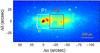 |
Fig. 1 B-band image of NGC 625 from the Ohio State University (OSU) Bright Spiral Galaxy Survey (Eskridge et al. 2002). The area covered in ESO programme 086.B-0042 is indicated with two squares (white for pointing 1, red for pointing 2). The scale for a distance of 3.9 Mpc is indicated in the lower right corner. The orientation is north (up) and east (to the left). |
2. Observations
Data were obtained in service mode during period 86 using the integral field unit of VIMOS (Le Fèvre et al. 2003) at Unit 3 (Melipal) of the Very Large Telescope (VLT). Both the HR_Blue and HR_Orange grisms were used. Their nominal spectral ranges are 4150–6200 Å and 5250–7400 Å, respectively, allowing coverage in a continuous manner from 4200 Å to 7200 Å. In these modes the field of view per pointing covers 27′′ × 27′′ with a magnification set to 0.̋67 per spatial element (hereafter, spaxel).
In order to fully map the area of the strongest level of star formation, a mosaic of two tiles was needed with an offset of 29.̋0 (i.e. 44 spaxels) in right ascension between them (see Fig. 1). For each tile, a square 4 pointing dither pattern with a relative offset of 2.̋7, equivalent to 4 spaxels, was used. It has been proved that this pattern is adequate to minimise the effect of dead fibers and therefore map continuously the area of interest (Arribas et al. 2008). Additionally after finishing the observation of each square pattern, a nearby sky background frame was obtained to evaluate and subtract the background emission. Standard sets of calibration files were also obtained. These included a set of continuum and arc lamps exposures. Each set of dither pattern, background, and standard calibration exposures constituted an observing block. Finally, spectrophotometric standards were also observed as part of the calibration plan of the observatory.
Atmospheric conditions during the observations were clear and the typical seeing ranged between 0.̋4 and 1.̋1. All the data were taken at low air masses to prevent strong effects due to differential atmospheric refraction. Nevertheless, as a safety test, the magnitude of these effects was checked a posteriori during the reduction process (see Sect. 3). Details about the utilised spectral range (shorter than the nominal one), resolving power, exposure time, airmass, and spectrophotometric standard for each pointing and configuration are shown in Table 2.
Observation log.
3. Data reduction
Data were procesed via the p3d tool (version 2.2, Sandin et al. 2010, 2011, 2012)1 and some IRAF2 routines. The p3d tool was utilised in the reduction of the individual exposures. The VIMOS data are provided in four files per detector that are reduced separately and combined after the flux calibration to create a file containing the full field with all 1600 spectra. Here is a description of the method.
As first steps, bias was subtracted and spectra were traced using the provided standard calibration files. Then, a dispersion mask per observing block was created using the available arc image. The residual r between the fitted wavelength and the known wavelengths of the arc lines was always in the range 0.02 ≲ r ≲ 0.06 Å.
In a fourth step, cosmic-ray hits are removed in the science images using the PyCosmic algorithm (Husemann et al. 2012).
The fifth step was the extraction of the spectra. With VIMOS, calculated profiles have to be offset due to differences in the instrument flexures between the three continuum lamp exposures and the science exposures. New centre positions are calculated (for working fibres) in the science images, which are first median-filtered on the dispersion axis. One median value of the difference between all old and new centre positions is calculated and added to the profile positions. After that, spectra are extracted using the multi-profile deconvolution method (Sharp & Birchall 2010). Data of all four quadrants of either grism are set up to use the same wavelength array. The dispersion mask was then applied in a sixth step.
To estimate the accuracy achieved in the wavelength calibration for the science frames we fitted the [O i]λ6300 sky line in each spectrum by a Gaussian for the data taken with the HR_Orange grism. The standard deviation of the distribution of centroids of the lines was ~ 0.02 Å. Assuming this is a proxy of the quality in the wavelength calibration, this implies an accuracy of ~1 km s-1. For the HR_Blue, the [O i]λ5577 was used. We also measured a standard deviation of ~ 0.02 Å.
Similarly, the width of the Gaussian can be used as a proxy of the spectral resolution. We measured a instrumental width σ ~ 0.75( ± 0.06) Å and ~ 0.69( ± 0.05) Å via the [O i]λ6300 and [O i]λ5577 lines, for the HR_Orange and HR_Blue grism configurations, respectively. This translates to σinstru ~ 36 km s-1 for both configurations.
In a seventh step, a correction to the fibre-to-fibre sensitivity variations was applied. To accomplish this, the spectra were divided by the mean spectrum of an extracted and normalised continuum lamp flat-field image made out of the combination of three continuum-lamp exposures, excluding all spectra of broken and low-transmission fibres. Then, extracted spectra were flux calibrated using the standard-star exposure of the respective night and grism.
The last step of the reduction of the individual exposures was the creation of a data cube by combining the flux calibrated images of the four separate detectors and reordering the individual spectra according to their position within the VIMOS-IFU.
After this reduction, measured fluxes of the telluric lines still showed some variations depending on both the detector and spatial elements per se (also see Lagerholm et al. 2012). All spectra within a data cube are therefore normalised to achieve the same integrated median flux in a telluric line. To accomplish this, we used the brightest observed line in each configuration (i.e. λ = 5577 Å and λ = 6300 Å with data of both HR_Blue and HR_Orange, respectively).
The p3d tool evaluates the offsets due to differential atmospheric refraction (DAR) using the expressions listed by Ciddor (1996) and offers the possibility of correcting for it as described in Sandin et al. (2012). In our specific case, these were always ≲0.2 spaxels and ≲0.3 spaxels for the utilised spectral range in the HR_Orange and HR_Blue configuration, respectively. Since this is relatively small and a correction for differential atmospheric refraction would imply an extra interpolation in the data, we took the decision of not applying such a correction.
After the cubes for the individual exposures were fully reduced, all science cubes in each observing block were combined using the offsets commanded to the telescope and the IRAF task imcombine. Then a high signal-to-noise background spectrum was created by combining the individual spectra of the background exposure and subtracted afterwards. Finally, the two resulting cubes for each HR_Blue pointing were combined.
4. Results
4.1. Pinpointing Wolf-Rayet emission
Rest-frame wavelength of the narrow filters proposed by Brinchmann et al. (2008).
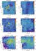 |
Fig. 2 Maps showing the location of the Wolf-Rayet features with respect to the overall stellar population. Left (right) column contains information for pointing 1 (2) (see Fig. 1). Upper row: maps for the blue bump emission are shown. Middle row: maps for the red bump emission are shown. Lower row: maps for a emission line free stellar continuum are shown. Every map shows contours tracing the observed Hα flux in steps of 0.3 dex as derived from Gaussian fitting (see Monreal-Ibero et al., in prep.). Likewise, utilised squared apertures to extract the spectra at the locations presenting W-R emission are shown and numbered in black. A cross at the peak of emission in Hα marks our origin of coordinates. The orientation is north up and east to the left. The colour bar on the right of each plot indicates the flux associated with the feature of interest in linear arbitrary units. |
To localise the W-R emission in NGC 625, narrow tunable filters were simulated using redshift of the galaxy and the bands proposed in Brinchmann et al. (2008), which are listed in Table 3 for completness. Depending on the characteristics of the stellar continuum, this very simple procedure may create flux maps with negative values at specific spatial elements. To avoid this, we added a common flux offset determined ad hoc to all spatial elements. This does not affect our purposes (i.e. identifying the locations with emission excess at the bumps). Then, following the methodology explained in Monreal-Ibero et al. (2011), we convolved the resulting image with a Gaussian of σ = 0.̋7 to better identify the places that might present W-R emission. The resulting maps for the blue and red bumps are presented in the first and second rows of Fig. 2. We set our origin of coordinates at the peak of emission in Hα. Additionally, a map to trace the overall stellar structure, made by simulating the action of a relatively broad filter (4400–4700 Å), decontaminated from any emission feature (see Paper II, in prep.), is presented in the third row. Likewise, to have a reference for the structure of the ionised gas, contours corresponding to the Hα emission are overplotted in each map. In short, these maps show that i) W-R emission in this galaxy is extended and with peaks of emission in multiple locations; ii) the peaks for the blue bump emission may or may not coincide with those of the red bump emission; and iii) these peaks, in general, do not necessarily coincide with either the overall general stellar or ionised gas emission distribution. Specifically, the stellar distribution presents several peaks of emission. The most important peak is associated with the peak of emission in Hα (contours in Fig. 2) and with the largest peak for the blue bump emission. Additionally, the overall stellar distribution present some peaks at  , which are associated with a plethora of young (i.e. ≲20 Myr) stars identified by means of HST broad band imaging (Cannon et al. 2003; McQuinn et al. 2012). However, no W-R emission in any of the bumps is seen there. In general, the blue bump emission is more concentrated than the red bump emission. Indeed the only W-R emission detected in P2 is in the red bump at about 400 pc from the peak of emission in Hα.
Those locations with eight3 or more adjacent spatial elements showing values 0.8 times standard deviations above the median of the whole image in at least one of the maps were identified as candidates with W-R emission whose spectra should be extracted to be analysed in more detail. The eight locations satisfying this criterion, as well as the square apertures that we used to extract the spectra, are numbered and marked in every map of Fig. 2. Their analysis is the subject of the next section.
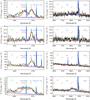 |
Fig. 3 Spectra in selected apertures presenting Wolf-Rayet features. The total modelled spectrum is shown in green whilst the fluxes corresponding to the W-R stellar features and nebular lines are shown in red and blue continuous lines, respectively, with a small offset. Additionally, individual fits for each feature are shown as dotted lines. The positions of the nebular emission lines are indicated with blue ticks and labels, whilst those corresponding to Wolf-Rayet features appear in red. Apertures were numbered according to decreasing right ascension and increasing declination. Their locations and sizes are shown in Fig. 2. |
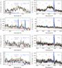 |
Fig. 3 continued. |
4.2. Composition of the Wolf-Rayet star population
4.2.1. Spectral fitting
Estimating the number of Wolf-Rayet stars in a given extragalactic spectrum is not straightforward. One typically depends on only one spectral feature (most likely the blue bump) or two at most to trace an assorted zoo of stars in terms of the existence, strength, and width of features in their spectra. The most popular strategy has probably been comparing the observed spectra with the predictions of models of stellar populations such as those presented by Schaerer & Vacca (1998).
The profiles of the extracted spectra for NGC 625 at the blue and red bumps are presented in Fig. 3. They are complex, showing a diversity of stellar features, pointing towards different W-R populations for the different apertures, on top of several nebular lines. Additionally, some sky background residuals for the Na id are also seen at 5893 Å. Although still limited to the use of only these two bumps, the quality (i.e. signal-to-noise and spectral resolution) of the spectra is good enough to attempt the more demanding, but more informative, approach of estimating the number of stars as a combination of templates for individual stars. In particular, since the metallicity of NGC 625 (see Table 1) is ~30% higher than that of the SMC and ~40% lower than that of the LMC (i.e. 12 + log (O / H) = 8.03 and 12 + log (O / H) = 8.35, respectively Russell & Dopita 1992), and the flux of the Wolf-Rayet features decreases with metallicity, we based our estimation on the results provided by Crowther & Hadfield (2006) for LMC and SMC Wolf-Rayet stars. One can, with our spectra, distinguish some of the different types of Wolf-Rayet stars. However, they are not (yet) comprehensive enough to disentangle all the different templates provided by Crowther & Hadfield (2006). Because of that, we ran different ensembles of fits, which were each based on only a subgroup of three templates: an early WN (i.e. WN2-4), a late(-ish) WN, which could be WN5-6 or WN7-9, and a “WC” (encompassing WC4 and WO). The different subsets of templates used are listed in Table 4. Crowther & Hadfield (2006) provide in their Tables 1 and 2 mean optical luminosities for the different stellar features including or excluding binaries. The fraction of binaries among the W-R for the SMC and the LMC is 40% and 30%, respectively (Foellmi et al. 2003a,b) and it is reasonable to expect a similar fraction for NGC 625. Thus, we used in our templates the mean fluxes when including binaries. The effects of using the mean values when including only single stars is discussed below.
Subsets of templates by Crowther & Hadfield (2006) used in the fits.
Results from spectra modelling and HST photometry.
The ingredients for the fits using a given set of templates were the following:
-
In addition to the stellar features, we included in the fit a 1-degpolynomial representing the emission of the underlying stellarpopulation and a set of nebular lines([Fe iii]λ4658, He iiλ4686, [Fe iii]λ4701, [Ar iv]+ He iλ4712, and [Ar iv]λ4740 in blue and [N ii]λ5755 and He iλ5876 in the red). They are marked with blue ticks in Fig. 3. The Mg i]λ4562.6 and Mg i]λ4571.0, clearly visible in apertures ♯1-♯3, were not included in the fit. Since they are too blue with respect to the blue bump, they did not have any major influence in our fitting technique. Nebular lines within each spectral range were linked in wavelength with an imposed width of σ = 0.7 Å for all of them. Flux was left as free parameter. We obtained an initial guess for the nebular line fluxes using splot within IRAF.
-
Stellar features were modelled by Gaussians with all the features in the blue bump having the same width. Given the complexity of the fits in the blue bump, this width was not a free parameter. Instead, we imposed a different value for each aperture aiming at reproducing the He ii line profile as best as possible. The assumed value for each aperture is shown in the second column of Table 5.
-
Firstly, we modelled the red bump with a single Gaussian centred at 5808 Å4. Its width was left free, and the flux could be an integer number of times (including 0) the fluxes provided in Table 2 of Crowther & Hadfield (2006), scaled at the distance of NGC 625 and assuming no intrinsic reddening for the galaxy (see Paper II, in prep.). We obtained a first estimation of the number of WC (or WO) stars from the model that minimised the χ2.
-
Secondly, we modelled the blue bump, using Gaussians representing the features of N vλ4610, N iiiλ4640, C iiiλ4647–4650/C ivλ4658 , and He iiλ4686. For the WC(WO) stars, Crowther & Hadfield (2006) give the global integrated flux of the last three features. After trying different relative ratios between the carbon and helium features, we adopted 0.8:0.2 as the most adequate ratio to reproduce the observed profiles. Then, we reproduced the flux of all these features as a combination of an integer number of WN and WC (or WO) stars, again allowing for non-detection of WN stars. While the number of WN stars was left free, for the number of WC(WO) we used the results for the red bump, allowing only for small variations in the number of stars. The model that minimised the χ2 gives an estimation of the number of stars for each type: early-type WN, late-type WN, and WC.
-
Thirdly, we compared the results from the blue and red bump, regarding the number of WC(WO) stars. Typically they were consistent (i.e. they gave a slightly different number of stars in only a few cases). The values presented in Table 5 refer to the number of stars derived from the fits in the blue bump. When these numbers differed, we checked that the predictions of the blue bump could also reasonably reproduce the red bump.
4.2.2. Caveats related to template selection
Since the metallicity of NGC 625 is between those of the SMC and LMC, we chose the most reasonable set of templates at each metallicity as the basis for the subsequent considerations. These were WN2-4bin/WN5-6/WObin for the SMC (subset D) and WN2-4/WN5-6/WC4bin for the LMC (subset A), where bin refers to templates with binary stars taken into consideration. The minimum χ2 was comparable when using any of the four subsets. Likewise, the spectral profiles were reproduced with similar accuracy. In the following, we discuss the subtleties associated with the use of other ensembles of templates and why we consider predictions using subsets A and D as the most reasonable.
Including or excluding binaries: studies on Galactic massive O stars indicate that an important fraction of these stars are in a state of binary interaction (e.g. Sana & Evans 2011; Kiminki & Kobulnicky 2012) and similar results have been reported for the Magellanic Clouds (Foellmi et al. 2003a,b). Therefore, our preferred subsets of templates were those for which observations of binaries stars were taken into account. However, when possible we also fitted the spectra via the templates made from observations of single stars only (ensembles not included in Table 4). Luminosities for the LMC templates are only slightly smaller and the number of stars estimated was the same independent of whether templates with or without binaries were used. When using SMC templates based on only single stars, the fits predict a number of WC ~ 1–2 larger, depending on the aperture, but an unrealistically large number of WN stars.
WC4 or WO as template for WC: as shown by Crowther et al. (1998) when moving from lower to higher excitation (i.e. ~WC4 to WO1), the ratio O vλ5590/C ivλ5808 should increase, being ≲0.01 for WC4 but ≲0.2 for WO4 (and even higher for earlier types). Whilst C ivλ5808 is clearly detected, there is no hint of O vλ5590 in our spectra. Therefore, the presence of WC4 stars over WO stars in NGC 625 is more reasonable. For models at the metallicity of the SMC, there are no WC4 templates available, so we had to use the templates for WO stars. For completeness, we fitted the spectra using the ensemble C, which includes the WO template for the LMC, even if we do not expect WO stars to be responsible of the observed spectra. Since fluxes for WO stars are smaller than for WC4 stars, this set of fits estimate typically up to three more times W-R stars, depending upon the aperture, than ensemble A.
WN5-6 or WN7-9 as template for late WN: this dilemma uniquely concerns the fitting using the LMC templates since no WN7-9 template for the SMC metallicity exists. Both types of stars present N vλ4610 and He iiλ4686, where the He ii line is ~6.7 (4.2) times stronger than the N v line for the WN5-6 (WN7-9) stars. In view of the spectra in Fig. 3, we do not expect to have WN7-9 in apertures ♯2 and ♯3. Likewise, spectrum in aperture ♯ 6 is not affected by this discussion, since it can be properly reproduced with only WC stars. Regarding apertures ♯1, ♯4, and ♯5, the blue bump is dominated by early-type WN stars, and considering the WN7-9 or the WN5-6 template as representative of late-type WN stars changes the total number of estimated W-R stars only marginally. Finally, because of their lower quality, the fits of the spectra in apertures ♯6 and ♯7 are not reliable and are very dependent on the used set of templates. However, for aperture ♯6, emission features are relatively narrow, supporting the existence of late-type WN stars in this aperture. For aperture ♯7, even if the spectrum is consistent with the existence of WN stars, it is not possible to discern a more refined classification with these data.
4.2.3. Adopted W-R numbers
The final number of stars per aperture is shown in Table 5 whilst the optimal fit to the spectrum profile when using the templates for the ensemble A is shown in Fig. 3 with a green line.
Interestingly, the assumed width for the features in the fits increases from aperture ♯6, continuing for all the other apertures up to aperture ♯8 tracing a sequence from apertures where the number of stars is dominated by late-type WN to those dominated by WC. This is very much in accord with the trend observed for individual stars, which typically present FWHM of ~15 Å for WN7-9, ~22 Å for WN5-6, ~30–60 Å for WN3-4, and up to ~70 Å for WC4 (Crowther & Hadfield 2006) and supports our method of disentangling the different types of W-R stars.
Figure 3 also shows that there is a clear detection of nebular He ii in two of the apertures, ♯2 and ♯3, both dominated by late-type WN stars. Additionally, there is marginal detection of nebular He ii in aperture ♯1. This is relevant since only certain classes of W-R stars, and maybe certain O stars, are predicted to be hot enough to ionise nebular He ii5 (Kudritzki 2002; Crowther et al. 2007). The analysis of this emission will be part of a forthcoming communication devoted to the analysis of the ionised gas (Paper II, in prep.).
Finally, it is worth noting that the spectral profiles for apertures ♯1 and ♯4 are not well reproduced. This might point towards an underestimation of the N v flux in the templates. Alternatively, it might call for a more refined modelling of the spectral profile than devised here. We envision two possible ways of improving the methodology presented here. On the one hand, the extraction of the spectra associated with W-R emission can be improved using more accurate methods than the use of square apertures as presented in Sect. 4.1. One possibility particularly promising for IFS data is extending the well-established concept of crowded field photometry in images into the domain of three-dimensional spectroscopic data cubes (Kamann et al. 2013). This has been proven to be extremely successful for disentangling the spectra of heavily blended stars (Husser et al. 2016). On the other hand, it is known that luminosities of the spectral features of a given W-R type spread over ≳2 orders of magnitudes. In that sense, fits could be improved by passing from the use mean templates per W-R type to a more refined grid of models, such as the Potsdam Wolf-Rayet Models6(PoWR; Hamann & Gräfener 2004; Todt et al. 2015; Sander et al. 2012). Already operating at the VLT, MUSE is able to provide higher quality data as those presented here in terms of depth and spatial resolution. Likewise, MEGARA at the GTC will collect IFS data at even higher spectral resolution. These and similar instruments will allow us to test these two methodologies.
In the following, we discuss our estimations of W-R star numbers with those found in galaxies at similar distances, model predictions, and with already published HST photometry for this galaxy. The discussion is based on the results obtained when using the ensembles A and D.
5. Discussion
5.1. Numbers of W-R stars
5.1.1. Comparison with published HST photometry
The method of estimating the number of W-R stars presented in the previous section represents a step forward with respect to the use of the integrated luminosity of one or two W-R features in the sense that it is able to estimate not only the number of W-R stars, but also the range of type. With the assumed luminosities for the templates, we estimate the existence of more than one star in most of the apertures that were unresolved at the VIMOS spatial resolution. Since W-R spectral features for a given type can vary ≳1–2 orders of magnitude in flux, from object to object (e.g. Crowther & Hadfield 2006), and the estimated numbers of stars depends largely of the used set of templates, it would be desirable to test with independent information whether the numbers of stars estimated in Sect. 4.2 are reasonable. In this way, we can evaluate whether LMC or SMC templates are more adequate to reproduce the W-R emission in NGC 625. An excellent option to accomplish this, would be the use of the already published high spatial resolution photometry with the HST for this object (Cannon et al. 2003; McQuinn et al. 2012)7. In this section, we correlate the location of our regions with W-R emission with the positions, V − I colours, and I magnitudes of the individual stars kindly provided by Dr. J. M. Cannon.
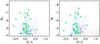 |
Fig. 4 Section of the HR diagrams for NGC 625 presented by McQuinn et al. (2012). Stars in the central part of the galaxy satisfying the criteria of MV< − 4.05 and − 1.0 <V − I< 0.6 are shown with blue dots. Those stars within the VIMOS apertures are shown with larger green circles. |
 |
Fig. 5 Section of the HST image of NGC 625 in F555W (programme 8708, P.I.: Skillman). All the stars in the central region of the galaxy that satisfy the criteria of MV< − 4.05 and − 1.0 <V − I< 0.6 are indicated with blue circles. Those falling within the apertures defined in Sect. 4.1 (red squares) are shown in thicker green circles. There is no available photometry for apertures ♯1 and ♯3. |
The aim is to quantify whether the number of W-R stars that we have estimated in Sect. 4.2 is compatible with the number of massive stars found at each location. This exercise needs accurate astrometry both in the HST images and VIMOS maps. We computed the best astrometric solution for the HST archive images by selecting ~40 stars with MI ≤ − 6.9 spread over the whole field of the WFPC2. We used ccmap within IRAF and allowed for shift and scaling in both directions as well as rotation. A few additional, slightly fainter, stars in the WF4 camera were also added.
Astrometry for the VIMOS-IFU maps was extremely difficult because of the relatively small field of view and the scarcity of point sources. For pointing 1, we correlated the five peaks of emission in the blue continuum maps with bright stars in a Gaussian-smoothed version of F555W HST image. Then we computed the astrometric solution assuming no rotation. For pointing 2, identifying enough point sources was not possible. Therefore, we utilised the solution found for pointing 1 and applied the offset commanded at the telescope.
Once the positions in the HST images and VIMOS-IFU maps are matched, one can count the number of massive stars in the selected apertures. Published MV magnitudes for W-R stars in SMC are always brighter than MV = − 4.05 (Bartzakos et al. 2001; Foellmi et al. 2003a). Therefore, we set this value as the lower limit for the MV magnitude of a putative W-R in NGC 625. Likewise, since W-R stars are blue, we restricted our search to stars with − 1.0 < (V − I) < − 0.6 colours. The position in the colour magnitude diagram for the stars in the central part of NGC 625 satisfying these two criteria is shown in Fig. 4, while the locations of the stars in the HST image are shown in Fig. 5 and the number of stars in each aperture are presented in the last column of Table 5. We do not include the numbers of massive stars in apertures ♯1 and ♯3 since there is no photometry available for them most likely owing to heavy crowding.
Regarding the other apertures, one would expect a number of massive stars, as found by means of HST photometry, which are larger or equal to the number of Wolf-Rayet stars, as estimated by means of the VIMOS spectroscopy. Taking the results using the set of templates A and D as baselines, the number of stars when using the LMC templates is consistent with the HST photometry. We estimate one additional star for aperture ♯5 but this is well within the uncertainties of the method. On the contrary, by using the SMC templates we estimate the same or much larger number of W-R stars, and therefore this estimate is incompatible with existing HST photometry. This is an interesting point. The metallicity of NGC 625 is closer to that of the SMC, and still modelling via the LMC templates gives more reasonable predictions in terms of number of W-R stars. This might point towards a non-linear relation between the metallicity and luminosity of the W-R features. Instead, it would present an elbow in the sense that luminosity declines faster at metallicities closer to that of the SMC. Further observations of a larger sample of W-R stars covering a diversity of metallicities would be necessary to test this possibility.
5.1.2. Comparison with nearby galaxies and model predictions
Likewise, it would be of interest to see how our predictions, using both LMC and SMC templates, compare with the W-R content in other galaxies at similar distances as NGC 625 as well as with the predictions of models. To accomplish this, in addition to the number of WN and WC stars, we need an estimation of the number of O stars. This was obtained by co-adding all the spectra in the VIMOS pointings with f(Hα)> 10-17 erg s-1 cm-2 and comparing the integrated Hα flux and equivalent width with the predictions of Starburst99 (Leitherer et al. 1999), assuming a distance for NGC 625 of 3.9 Mpc (see Table 1) and no extinction intrinsic to the galaxy (Monreal-Ibero et al., in prep.). To be specific, the integrated spectrum was made of the sum of 2481 spectra, which at the distance of NGC 625 corresponds to an area of 0.398 kpc2, and had an integrated Hα flux of f(Hα)int ~ 4.26 × 10⁻¹² erg s-1 cm-2 and an equivalent width, EW(Hα) = 150 Å. We used the original Starburst99 models with metallicities Z = 0.008 (LMC) and Z = 0.004 (SMC) and assuming a Salpeter initial mass function (i.e. α = 2.35) with Mup = 100M⊙. We also assumed an instantaneous burst of star formation. The estimated number of O stars and the WC/WN and WR/O ratios are presented in Table 5.
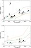 |
Fig. 6 Relative number of WC to WN stars (top) and WR to O stars (bottom) for NGC 625. Predictions when using the templates for the LMC (subset A) are indicated with a filled blue star while whose using the SMC templates (subset D) are indicated with an empty red star. Two vertical lines of these same colours indicate the metallicity of the templates. We included for comparison the prediction of the models by Eldridge et al. (2008) for binary and single stars (thick and thin green lines, respectively) as well as models by Meynet & Maeder (2005) for stars with rotation (v = 300 km s-1) and without rotation (thick and thin orange lines, respectively). Likewise W-R star content for other very nearby galaxies has been added for reference: NGC 7793, Bibby & Crowther (2010); NGC 5068, Bibby & Crowther (2012); M 31, Neugent et al. (2012); M 33, Neugent & Massey (2011); NGC 1313, Hadfield & Crowther (2007); LMC, Massey et al. (2015); SMC Massey et al. (2014); IC 10, Crowther et al. (2003); and NGC 300, Crowther et al. (2007). |
Those ratios when using the set of templates A and D are shown in Fig. 6 together with the estimated W-R content for galaxies at similar distances. Likewise, we superimposed the predictions from the models by Meynet & Maeder (2005) and the Binary Population and Spectral Synthesis8 (BPASS; Eldridge et al. 2008) to address the role of rotation and existence of binary stars. The proportion of WC to WN is comparably independent of the used set of templates and of the order of the proportions found for galaxies at similar metallicities, with the exception of IC 10 for which an anomalous N(WC)/N(WN) ratio has already been reported (Royer et al. 2001). Also, at the metallicity of NGC 625 the model predictions are fairly similar, and thus they do not allow us to favor binary stars versus rotation (see Fig. 6). However, independent of the set of used templates, our N(WC)/N(WN) ratio is clearly compatible with model predictions, again supporting the approach presented in Sect. 4.
The lower graphic in Fig. 6 shows our estimated proportions of O versus W-R stars. The predictions are different by a factor of ~7 depending on whether we use the templates for the LMC or for the SMC. Our estimation using the LMC templates is much more in agreement with model predictions and with the only galaxy at similar metallicities (i.e. NGC 1313), than that using the SMC templates. This again supports the hypothesis of a non-linear relation between the metallicity of the star and the luminosity of the W-R features.
All in all, the most reasonable estimation for the W-R content in NGC 625 is that obtained when using the LMC templates (subset A). We estimate a total of 28 W-R stars in the galaxy, out of which, 17 are early-type WN, six are late-type WN, and five are WC stars.
5.2. Wolf-Rayet star population and the spatially resolved star formation history in NGC 625
Given their short duration, Wolf-Rayet stars can pinpoint at a very detailed level the moment and location where recent star formation has taken place, and thus trace how this propagates through the galaxy. In principle, if a star passes through a W-R phase, the WN stage precedes the WC stage (Crowther et al. 2007). For the more refined classification used here, we can consider a “baseline” evolutionary path O star → late-type WN → early-type WN → WC. Details and temporal scales for an individual star would depend on its mass, metallicity, amount of rotation, whether it is a binary or not, etc., with multiple variations of this baseline. For example, some stars might not necessarily become WC stars whilst others might suffer LBV episodes. The relevant point here is that roughly speaking, one would expect WN stars to be present predominantly in the younger regions, whilst WC stars should be expected in somewhat older regions (Westmoquette et al. 2013).
According to the results presented in Table 5, aperture ♯8 (towards the west and the furthest from the peak of emission in Hα) contains only one WC star. In contrast, apertures ♯1, ♯5, and ♯4 (closer to the peak of emission) contain a mix of WC and early WN stars. Aperture ♯7 contains star(s) of type WN. Finally apertures ♯2, ♯3, and ♯6 contain only WN and are dominated by late-type WN with only one early-type WN in aperture ♯3, which is the one centred at the peak of emission in both Hα and the stellar continuum, and aperture ♯6 is associated with one of the strongest H ii regions in the galaxy (NGC 625 B, in the nomenclature used by Cannon & Skillman 2004). Thus, the W-R population would suggest that star formation has propagated from the western and more external parts of the galaxy inwards with most recent star formation at the peak of emission. This is a crude map of the propagation of the star formation, but is roughly compatible with the findings using high spatial resolution imaging with the WFPC2/HST (Cannon et al. 2003; McQuinn et al. 2012).
In this context, one would expect no WR feature or only a WC star signature in the other brightest region in the galaxy (NGC 625 C in the nomenclature used by Cannon & Skillman 2004). In that sense, the non-detection of WR features at this location is reasonable. However, to check whether the lack of detection of W-R features in this location was an effect of our imposed threshold for the detection of the bumps, we extracted the spectrum associated with this region. It did not show any strong sign of blue or red bumps. This nicely supports the interpretation presented above even if this does not reject the possibility of existence of a few W-R stars at this location with line fluxes that are lower than the average (which is what it is considered in the templates).
Likewise, an alternative (or complementary) scenario to explain why the W-R star identified in aperture ♯8 has been found that far from the rest of the W-R population is the possibility that it is a runaway star. One of the two main proposed mechanisms by which a star can be ejected from its birthplace are the supernova explosions. NGC 625 actually displays non-thermal synchrotron radiation in one of its main H ii regions (NGC 625 C in the nomenclature used by Cannon & Skillman 2004), which is at ~250 pc north-east of our aperture ♯8. Supernova remnants can be detected in the radio for up to ~ 105 yr (Bozzetto et al. 2017). Thus, independent of the age of the WC star, if we assume that the supernova was the agent causing the star to run away, then an extremely large kick velocity would be needed for the star to reach is current location. Therefore, the dynamical ejection scenario, whereby the ejection is caused by encounters in a dense cluster appears to be more plausible. In this scenario, and assuming an age of ~ 5 Myr for the WC star in this aperture, a kick velocity of ~ 50 km -1 would have been enough for the star to reach its current location. Alternatively, the star could come from the largest H ii region at ~400 pc, if we take as reference the peak of emission in Hα. For the distance between the WC star and the H ii region and assuming a similar age or somewhat younger (~ 3–5 Myr), the kick velocity would be ~ 80–130 km s-1. These are all within the range of velocities for runaway stars suggested by Rosslowe & Crowther (2015).
6. Conclusions
We have carried out a detailed study of the central ~ 1100 × 550 pc of the nearby BCD NGC 625 with VIMOS-IFU observations. In this paper, we present the data and discuss the W-R star population. Our main conclusions can be summarised as follows:
-
1.
The Wolf-Rayet star population is spread over the main body ofthe galaxy and does not necessarily coincide with the overallstellar structure. Likewise, while the blue bump emission, whichis characteristic of WN stars, is more concentrated with amaximum at the peak of emission in both continuum and Hα, the redbump emission is more extended and peaks
 north. Indeed, WC emission has been detected at
distances up to 400 pc from the peak of emission in continuum and Hα.
north. Indeed, WC emission has been detected at
distances up to 400 pc from the peak of emission in continuum and Hα. -
2.
Nebular He ii has clearly been detected in two of the apertures, ♯2 and ♯3, which are the two dominated by late-type WN stars. Additionally, there is marginal detection of nebular He ii in aperture ♯1.
-
3.
The best estimation for the W-R content in NGC 625 is that obtained when using the LMC templates (subset A). We estimate a total of 28 W-R stars in the galaxy, out of which, 17 (61%) are early-type WN, six (21%) are late-type WN, and five (18%) are WC stars. Most of these (36%) are located in aperture ♯4 at
north from the peak of emission in continuum and
Hα.
-
4.
The width of the stellar features is correlated with the type of W-R stars found in each aperture, tracing a sequence from those apertures dominated by late-type WN stars, which present narrower features, to those dominated by WC stars, which have broader features. This is very much in accord with the trend observed for individual stars.
-
5.
Comparisons of our results with HST high spatial resolution photometry, with the W-R content in galaxies at similar distances and metallicites, and with the prediction of stellar evolutionary models indicates that modelling using LMC templates gives a more reasonable number of W-R stars than using SMC templates. However, the metallicity of the galaxy is closer to that of the SMC. This suggests that the relation between metallicity and luminosity of the W-R spectral features is non-linear with a steep decline at lower luminosities.
-
6.
The distribution of the different types of WR in the galaxy is roughly compatible with the way star formation has propagated in the galaxy, according to previous findings using high spatial resolution with the HST.
All papers are freely available at the p3d project web site http://p3d.sf.net
The Image Reduction and Analysis Facility, IRAF, is distributed by the National Optical Astronomy Observatories which is operated by the association of Universities for Research in Astronomy, Inc. under cooperative agreement with the National Science Foundation.
This would correspond to an area equivalent to that of a circle with  , comparable to the seeing of these observations.
All the wavelengths mentioned in this section are rest frame.
Ionisation potential: hν = 54.4 eV.
Programme 8708, P.I.: Skillman.
Acknowledgments
We thank John M. Cannon and Kristy McQuinn for making the HST photometry of NGC 625 available to us. We also thank the referee for useful comments that have significantly improved the first submitted version of this paper. Based on observations carried out at the European Southern Observatory, Paranal (Chile), programme 086.B-0042. A.M.-I. grateful to ESO Garching, where part of this work was carried out, for their hospitality and funding via their visitor programme. A.M.-I. acknowledges support from the Spanish PNAYA through project AYA2015-68217-P and from BMBF through the Erasmus-F project (grant number 05 A12BA1). M. R. acknowledges support by the research projects AYA2014-53506-P from the Spanish Minister de Economía y Competitividad, from the European Regional Development Funds (FEDER) and the Junta de Andalucía (Spain) grants FQM108.
This paper uses the plotting package jmaplot9, developed by Jesús Maíz-Apellániz. This research made use of the NASA/IPAC Extragalactic Database (NED), which is operated by the Jet Propulsion Laboratory, California Institute of Technology, under contract with the National Aeronautics and Space Administration.
References
- Allen, D. A., Wright, A. E., & Goss, W. M. 1976, MNRAS, 177, 91 [NASA ADS] [Google Scholar]
- Armus, L., Heckman, T. M., & Miley, G. K. 1988, ApJ, 326, L45 [NASA ADS] [CrossRef] [Google Scholar]
- Arribas, S., Colina, L., Monreal-Ibero, A., et al. 2008, A&A, 479, 687 [NASA ADS] [CrossRef] [EDP Sciences] [Google Scholar]
- Bartzakos, P., Moffat, A. F. J., & Niemela, V. S. 2001, MNRAS, 324, 18 [NASA ADS] [CrossRef] [Google Scholar]
- Bastian, N., Emsellem, E., Kissler-Patig, M., & Maraston, C. 2006, A&A, 445, 471 [NASA ADS] [CrossRef] [EDP Sciences] [Google Scholar]
- Bibby, J. L., & Crowther, P. A. 2010, MNRAS, 405, 2737 [NASA ADS] [Google Scholar]
- Bibby, J. L., & Crowther, P. A. 2012, MNRAS, 420, 3091 [NASA ADS] [CrossRef] [Google Scholar]
- Bozzetto, L. M., Filipović, M. D., Vukotić, B., et al. 2017, ApJS, 230, 2 [NASA ADS] [CrossRef] [Google Scholar]
- Brinchmann, J., Kunth, D., & Durret, F. 2008, A&A, 485, 657 [NASA ADS] [CrossRef] [EDP Sciences] [Google Scholar]
- Cannon, J. M., & Skillman, E. D. 2004, ApJ, 610, 772 [NASA ADS] [CrossRef] [Google Scholar]
- Cannon, J. M., Dohm-Palmer, R. C., Skillman, E. D., et al. 2003, AJ, 126, 2806 [NASA ADS] [CrossRef] [Google Scholar]
- Cannon, J. M., McClure-Griffiths, N. M., Skillman, E. D., & Côté, S. 2004, ApJ, 607, 274 [NASA ADS] [CrossRef] [Google Scholar]
- Ciddor, P. E. 1996, Appl. Opt., 35, 1566 [NASA ADS] [CrossRef] [PubMed] [Google Scholar]
- Conti, P. S. 1975, Mem. Soc. Roy. Sci. Liège, 9, 193 [Google Scholar]
- Conti, P. S. 1991, ApJ, 377, 115 [NASA ADS] [CrossRef] [Google Scholar]
- Crowther, P. A. 2007, ARA&A, 45, 177 [NASA ADS] [CrossRef] [Google Scholar]
- Crowther, P. A., & Bibby, J. L. 2009, A&A, 499, 455 [NASA ADS] [CrossRef] [EDP Sciences] [Google Scholar]
- Crowther, P. A., & Hadfield, L. J. 2006, A&A, 449, 711 [NASA ADS] [CrossRef] [EDP Sciences] [Google Scholar]
- Crowther, P. A., De Marco, O., & Barlow, M. J. 1998, MNRAS, 296, 367 [NASA ADS] [CrossRef] [Google Scholar]
- Crowther, P. A., Drissen, L., Abbott, J. B., Royer, P., & Smartt, S. J. 2003, A&A, 404, 483 [NASA ADS] [CrossRef] [EDP Sciences] [Google Scholar]
- Crowther, P. A., Carpano, S., Hadfield, L. J., & Pollock, A. M. T. 2007, A&A, 469, L31 [NASA ADS] [CrossRef] [EDP Sciences] [Google Scholar]
- de Vaucouleurs, G., de Vaucouleurs, A., Corwin, Jr., H. G., et al. 1991, Third Reference Catalogue of Bright Galaxies. Volume I: Explanations and references. Volume II: Data for galaxies between 0h and 12h. Volume III: Data for galaxies between 12h and 24h [Google Scholar]
- Dray, L. M., & Tout, C. A. 2003, MNRAS, 341, 299 [NASA ADS] [CrossRef] [Google Scholar]
- Drissen, L., Roy, J.-R., Moffat, A. F. J., & Shara, M. M. 1999, AJ, 117, 1249 [NASA ADS] [CrossRef] [Google Scholar]
- Eskridge, P. B., Frogel, J. A., Pogge, R. W., et al. 2002, ApJS, 143, 73 [NASA ADS] [CrossRef] [Google Scholar]
- Eldridge, J. J., Izzard, R. G., & Tout, C. A. 2008, MNRAS, 384, 1109 [NASA ADS] [CrossRef] [Google Scholar]
- Fernandes, I. F., de Carvalho, R., Contini, T., & Gal, R. R. 2004, MNRAS, 355, 728 [NASA ADS] [CrossRef] [Google Scholar]
- Foellmi, C., Moffat, A. F. J., & Guerrero, M. A. 2003a, MNRAS, 338, 360 [NASA ADS] [CrossRef] [Google Scholar]
- Foellmi, C., Moffat, A. F. J., & Guerrero, M. A. 2003b, MNRAS, 338, 1025 [NASA ADS] [CrossRef] [Google Scholar]
- Gil de Paz, A., Madore, B. F., & Pevunova, O. 2003, ApJS, 147, 29 [NASA ADS] [CrossRef] [Google Scholar]
- Hadfield, L. J., & Crowther, P. A. 2007, MNRAS, 381, 418 [NASA ADS] [CrossRef] [Google Scholar]
- Hamann, W.-R., & Gräfener, G. 2004, A&A, 427, 697 [NASA ADS] [CrossRef] [EDP Sciences] [Google Scholar]
- Husemann, B., Kamann, S., Sandin, C., et al. 2012, A&A, 545, A137 [NASA ADS] [CrossRef] [EDP Sciences] [Google Scholar]
- Husser, T.-O., Kamann, S., Dreizler, S., et al. 2016, A&A, 588, A148 [NASA ADS] [CrossRef] [EDP Sciences] [Google Scholar]
- Izotov, Y. I., Foltz, C. B., Green, R. F., Guseva, N. G., & Thuan, T. X. 1997, ApJ, 487, L37 [NASA ADS] [CrossRef] [Google Scholar]
- Jarrett, T. H., Chester, T., Cutri, R., Schneider, S. E., & Huchra, J. P. 2003, AJ, 125, 525 [NASA ADS] [CrossRef] [Google Scholar]
- Kamann, S., Wisotzki, L., & Roth, M. M. 2013, A&A, 549, A71 [NASA ADS] [CrossRef] [EDP Sciences] [Google Scholar]
- Karachentsev, I. D., Grebel, E. K., Sharina, M. E., et al. 2003, A&A, 404, 93 [NASA ADS] [CrossRef] [EDP Sciences] [Google Scholar]
- Kehrig, C., Perez-Montero, E., Vilchez, J. M., et al. 2013, MNRAS, 432, 2731 [NASA ADS] [CrossRef] [Google Scholar]
- Kiminki, D. C., & Kobulnicky, H. A. 2012, ApJ, 751, 4 [NASA ADS] [CrossRef] [Google Scholar]
- Kirby, E. M., Jerjen, H., Ryder, S. D., & Driver, S. P. 2008, AJ, 136, 1866 [NASA ADS] [CrossRef] [Google Scholar]
- Kudritzki, R. P. 2002, ApJ, 577, 389 [NASA ADS] [CrossRef] [Google Scholar]
- Lagerholm, C., Kuntschner, H., Cappellari, M., et al. 2012, A&A, 541, A82 [NASA ADS] [CrossRef] [EDP Sciences] [Google Scholar]
- Le Fèvre, O., Saisse, M., Mancini, D., et al. 2003, in SPIE Conf. Ser. 4841, eds. M. Iye & A. F. M. Moorwood, 1670 [Google Scholar]
- Lee, J. C., Gil de Paz, A., Kennicutt, Jr., R. C., et al. 2011, ApJS, 192, 6 [NASA ADS] [CrossRef] [Google Scholar]
- Leitherer, C., Schaerer, D., Goldader, J. D., et al. 1999, ApJS, 123, 3 [NASA ADS] [CrossRef] [Google Scholar]
- Lípari, S., Terlevich, R., Díaz, R. J., et al. 2003, MNRAS, 340, 289 [NASA ADS] [CrossRef] [Google Scholar]
- López-Sánchez, Á. R., & Esteban, C. 2010, A&A, 516, A104 [NASA ADS] [CrossRef] [EDP Sciences] [Google Scholar]
- Maeder, A. 1992, A&A, 264, 105 [NASA ADS] [Google Scholar]
- Marlowe, A. T., Meurer, G. R., Heckman, T. M., & Schommer, R. 1997, ApJS, 112, 285 [NASA ADS] [CrossRef] [Google Scholar]
- Massey, P., Neugent, K. F., Morrell, N., & Hillier, D. J. 2014, ApJ, 788, 83 [NASA ADS] [CrossRef] [Google Scholar]
- Massey, P., Neugent, K. F., & Morrell, N. 2015, ApJ, 807, 81 [NASA ADS] [CrossRef] [Google Scholar]
- McQuinn, K. B. W., Skillman, E. D., Cannon, J. M., et al. 2010, ApJ, 724, 49 [NASA ADS] [CrossRef] [Google Scholar]
- McQuinn, K. B. W., Skillman, E. D., Dalcanton, J. J., et al. 2012, ApJ, 759, 77 [NASA ADS] [CrossRef] [Google Scholar]
- Meynet, G., & Maeder, A. 2005, A&A, 429, 581 [NASA ADS] [CrossRef] [EDP Sciences] [Google Scholar]
- Miralles-Caballero, D., Díaz, A. I., López-Sánchez, Á. R., et al. 2016, A&A, 592, A105 [NASA ADS] [CrossRef] [EDP Sciences] [Google Scholar]
- Monreal-Ibero, A., Vílchez, J. M., Walsh, J. R., & Muñoz-Tuñón, C. 2010, A&A, 517, A27 [NASA ADS] [CrossRef] [EDP Sciences] [Google Scholar]
- Monreal-Ibero, A., Relaño, M., Kehrig, C., et al. 2011, MNRAS, 413, 2242 [NASA ADS] [CrossRef] [Google Scholar]
- Neugent, K. F., & Massey, P. 2011, ApJ, 733, 123 [NASA ADS] [CrossRef] [Google Scholar]
- Neugent, K. F., Massey, P., & Georgy, C. 2012, ApJ, 759, 11 [NASA ADS] [CrossRef] [Google Scholar]
- Phillips, A. C., & Conti, P. S. 1992, ApJ, 395, L91 [NASA ADS] [CrossRef] [Google Scholar]
- Relaño, M., Monreal-Ibero, A., Vílchez, J. M., & Kennicutt, R. C. 2010, MNRAS, 402, 1635 [NASA ADS] [CrossRef] [Google Scholar]
- Rosslowe, C. K., & Crowther, P. A. 2015, MNRAS, 447, 2322 [NASA ADS] [CrossRef] [Google Scholar]
- Royer, P., Smartt, S. J., Manfroid, J., & Vreux, J.-M. 2001, A&A, 366, L1 [NASA ADS] [CrossRef] [EDP Sciences] [Google Scholar]
- Russell, S. C., & Dopita, M. A. 1992, ApJ, 384, 508 [NASA ADS] [CrossRef] [Google Scholar]
- Sana, H., & Evans, C. J. 2011, in Active OB Stars: Structure Evolution, Mass Loss, and Critical Limits, IAU Symp. 272, eds. C. Neiner, G. Wade, G. Meynet, & G. Peters, 474 [Google Scholar]
- Sander, A., Hamann, W.-R., & Todt, H. 2012, A&A, 540, A144 [NASA ADS] [CrossRef] [EDP Sciences] [Google Scholar]
- Sanders, D. B., Mazzarella, J. M., Kim, D.-C., Surace, J. A., & Soifer, B. T. 2003, AJ, 126, 1607 [Google Scholar]
- Sandin, C., Becker, T., Roth, M. M., et al. 2010, A&A, 515, A35 [NASA ADS] [CrossRef] [EDP Sciences] [Google Scholar]
- Sandin, C., Weilbacher, P., Streicher, O., Walcher, C. J., & Roth, M. M. 2011, The Messenger, 144, 13 [NASA ADS] [Google Scholar]
- Sandin, C., Weilbacher, P., Tabataba-Vakili, F., Kamann, S., & Streicher, O. 2012, in Software and Cyberinfrastucture for Astronomy II, SPIE Conf. Ser., 8451, 84510F [Google Scholar]
- Schaerer, D., & Vacca, W. D. 1998, ApJ, 497, 618 [NASA ADS] [CrossRef] [Google Scholar]
- Schaerer, D., Contini, T., & Pindao, M. 1999, A&AS, 136, 35 [NASA ADS] [CrossRef] [EDP Sciences] [Google Scholar]
- Schlafly, E. F., & Finkbeiner, D. P. 2011, ApJ, 737, 103 [NASA ADS] [CrossRef] [Google Scholar]
- Sharp, R., & Birchall, M. N. 2010, PASA, 27, 91 [NASA ADS] [CrossRef] [Google Scholar]
- Skillman, E. D., Côté, S., & Miller, B. W. 2003, AJ, 125, 610 [NASA ADS] [CrossRef] [Google Scholar]
- Smartt, S. J. 2009, ARA&A, 47, 63 [NASA ADS] [CrossRef] [Google Scholar]
- Thuan, T. X., & Martin, G. E. 1981, ApJ, 247, 823 [NASA ADS] [CrossRef] [Google Scholar]
- Todt, H., Sander, A., Hainich, R., et al. 2015, A&A, 579, A75 [NASA ADS] [CrossRef] [EDP Sciences] [Google Scholar]
- Westmoquette, M. S., James, B., Monreal-Ibero, A., & Walsh, J. R. 2013, A&A, 550, A88 [NASA ADS] [CrossRef] [EDP Sciences] [Google Scholar]
- Woosley, S. E., & Bloom, J. S. 2006, ARA&A, 44, 507 [NASA ADS] [CrossRef] [Google Scholar]
All Tables
Rest-frame wavelength of the narrow filters proposed by Brinchmann et al. (2008).
All Figures
|
Fig. 1 B-band image of NGC 625 from the Ohio State University (OSU) Bright Spiral Galaxy Survey (Eskridge et al. 2002). The area covered in ESO programme 086.B-0042 is indicated with two squares (white for pointing 1, red for pointing 2). The scale for a distance of 3.9 Mpc is indicated in the lower right corner. The orientation is north (up) and east (to the left). |
| In the text | |
|
Fig. 2 Maps showing the location of the Wolf-Rayet features with respect to the overall stellar population. Left (right) column contains information for pointing 1 (2) (see Fig. 1). Upper row: maps for the blue bump emission are shown. Middle row: maps for the red bump emission are shown. Lower row: maps for a emission line free stellar continuum are shown. Every map shows contours tracing the observed Hα flux in steps of 0.3 dex as derived from Gaussian fitting (see Monreal-Ibero et al., in prep.). Likewise, utilised squared apertures to extract the spectra at the locations presenting W-R emission are shown and numbered in black. A cross at the peak of emission in Hα marks our origin of coordinates. The orientation is north up and east to the left. The colour bar on the right of each plot indicates the flux associated with the feature of interest in linear arbitrary units. |
| In the text | |
|
Fig. 3 Spectra in selected apertures presenting Wolf-Rayet features. The total modelled spectrum is shown in green whilst the fluxes corresponding to the W-R stellar features and nebular lines are shown in red and blue continuous lines, respectively, with a small offset. Additionally, individual fits for each feature are shown as dotted lines. The positions of the nebular emission lines are indicated with blue ticks and labels, whilst those corresponding to Wolf-Rayet features appear in red. Apertures were numbered according to decreasing right ascension and increasing declination. Their locations and sizes are shown in Fig. 2. |
| In the text | |
|
Fig. 3 continued. |
| In the text | |
|
Fig. 4 Section of the HR diagrams for NGC 625 presented by McQuinn et al. (2012). Stars in the central part of the galaxy satisfying the criteria of MV< − 4.05 and − 1.0 <V − I< 0.6 are shown with blue dots. Those stars within the VIMOS apertures are shown with larger green circles. |
| In the text | |
|
Fig. 5 Section of the HST image of NGC 625 in F555W (programme 8708, P.I.: Skillman). All the stars in the central region of the galaxy that satisfy the criteria of MV< − 4.05 and − 1.0 <V − I< 0.6 are indicated with blue circles. Those falling within the apertures defined in Sect. 4.1 (red squares) are shown in thicker green circles. There is no available photometry for apertures ♯1 and ♯3. |
| In the text | |
|
Fig. 6 Relative number of WC to WN stars (top) and WR to O stars (bottom) for NGC 625. Predictions when using the templates for the LMC (subset A) are indicated with a filled blue star while whose using the SMC templates (subset D) are indicated with an empty red star. Two vertical lines of these same colours indicate the metallicity of the templates. We included for comparison the prediction of the models by Eldridge et al. (2008) for binary and single stars (thick and thin green lines, respectively) as well as models by Meynet & Maeder (2005) for stars with rotation (v = 300 km s-1) and without rotation (thick and thin orange lines, respectively). Likewise W-R star content for other very nearby galaxies has been added for reference: NGC 7793, Bibby & Crowther (2010); NGC 5068, Bibby & Crowther (2012); M 31, Neugent et al. (2012); M 33, Neugent & Massey (2011); NGC 1313, Hadfield & Crowther (2007); LMC, Massey et al. (2015); SMC Massey et al. (2014); IC 10, Crowther et al. (2003); and NGC 300, Crowther et al. (2007). |
| In the text | |
Current usage metrics show cumulative count of Article Views (full-text article views including HTML views, PDF and ePub downloads, according to the available data) and Abstracts Views on Vision4Press platform.
Data correspond to usage on the plateform after 2015. The current usage metrics is available 48-96 hours after online publication and is updated daily on week days.
Initial download of the metrics may take a while.