© ESO, 2017

1. Introduction

Twenty years after the discovery of the first exoplanet around a Solar-type star (Mayor & Queloz 1995), the population of detected low-mass extra-solar planets has grown rapidly. Their number is now considerable and will keep increasing. This generates a strong need for theoretical modelling and predictions. Because the mass of such planets is not large enough to allow them to accrete a voluminous gaseous envelope, they are mainly composed of a telluric core. In many cases (e.g. 55 Cnc e, see Demory et al. 2016), this core is covered by a thin atmospheric layer as is observed on the Earth, Venus and Mars. The rotation of these bodies strongly affects their surface temperature equilibrium and atmospheric global circulation (Forget & Leconte 2014). Therefore, it is a key quantity to understand their climate, particularly in the so-called habitable zone (Kasting et al. 1993) where some of them have been found (Kopparapu et al. 2014).

The rotational dynamics of super-Venus and Venus-like planets is driven by the tidal torques exerted both on the rocky and atmospheric layers (see Correia et al. 2008). The solid torque, which is induced by the gravitational tidal forcing of the host star, tends to despin the planet to pull it back to synchronization. The atmospheric torque is the sum of two contributions. The first one, caused by the gravitational tidal potential of the star, acts on the spin in a similar way to the solid tide. The second one, called the “thermal tide”, results from the perturbation due to the heating of the atmosphere by the stellar bolometric flux. The torque induced by this component is in opposition to those gravitationally generated. Therefore, it pushes the angular velocity of the planet away from synchronization. Although the mass of the atmosphere often represents a negligible fraction of the mass of the planet (denoting f_A this fraction, we have f_A ~ 10^-4 for Venus), thermal tides can be of the same order of magnitude and even stronger than solid tides (Dobrovolskis & Ingersoll 1980).

This competition naturally gives rise to prograde and retrograde rotation equilibria in the semi-major axis range defined by the habitable zone, in which Venus-like planets are submitted to gravitational and thermal tides of comparable intensities (Gold & Soter 1969; Dobrovolskis & Ingersoll 1980; Correia & Laskar 2001). Early studies of this effect were based on analytical models developed for the Earth (e.g. Chapman & Lindzen 1970) that show a singularity at synchronisation, while Correia & Laskar (2001) avoid this weak point by a smooth interpolation annulling the torque at synchronization. Only recently, the atmospheric tidal perturbation has been computed numerically with global circulation models (GCM; Leconte et al. 2015), and analytically by Auclair-Desrotour et al. (2017, hereafter referred to as P1), who generalized the reference work of Chapman & Lindzen (1970) by including the dissipative processes (radiation, thermal diffusion) that regularize the behaviour of the atmospheric tidal torque at the synchronization.

Here, we revisit the equilibrium rotation of super-Earth planets based on the atmospheric tides model presented in P1. For the solid torque, we use the simplest physical prescription, a Maxwell model (Remus et al. 2012; Correia et al. 2014), because the rheology of these planets is unknown.

2. Tidal torques

2.1. Physical set-up

For simplicity, we considered a planet in a circular orbit of radius a and mean motion n around a star of mass M_∗ and luminosity L_∗ exerting on the planet thermal and gravitational tidal forcing (Fig. 1). The planet, of mass M_P and spin Ω, has zero obliquity so that the tidal frequency is σ = 2ω, where ω = Ω−n. It is composed of a telluric core of radius R covered by a thin atmospheric layer of mass M_A = f_AM_P and pressure height scale H such that H ≪ R. This fluid layer is assumed to be homogeneous in composition, of specific gas constant ℛ_A = ℛ_GP/m (ℛ_GP and m being the perfect gas constant and the mean molar mass respectively), in hydrostatic equilibrium and subject to convective instability, that is, N ≈ 0, with N designating the Brunt-Väisälä frequency, as observed on the surface of Venus (Seiff et al. 1980). Hence, the pressure height scale is $\mathit{H}\mathrm{=}\frac{{\mathrm{ℛ}}_{\mathrm{A}}{\mathit{T}}_{\mathrm{0}}}{\mathit{g}}\mathit{,}$(1)where T₀ is the equilibrium surface temperature of the atmosphere and g the surface gravity which are related to the equilibrium radial distributions of density ρ₀ and pressure p₀ as p₀ = ρ₀gH. We introduce the first adiabatic exponent of the gas Γ₁ = (∂lnp₀/∂lnρ₀)_S (the subscript S being the specific macroscopic entropy) and the parameter κ = 1−1/Γ₁. The radiative losses of the atmosphere, treated as a Newtonian cooling, lead us to define a radiative frequency σ₀, given by ${\mathit{J}}_{\mathrm{rad}}\mathrm{=}{\mathit{C}}_{\mathit{p}}{\mathit{\sigma }}_{\mathrm{0}}\mathit{\delta T,}$(2)where C_p = ℛ_A/κ is the thermal capacity of the atmosphere per unit mass and J_rad is the radiated power per unit mass caused by the temperature variation δT around the equilibrium state. We note here that the Newtonian cooling describes the radiative losses of optically thin atmospheres, where the radiative transfers between layers can be ignored. We applied this modelling to optically thick atmosphere, such as Venus’, because the numerical simulations by Leconte et al. (2015) show that it can also describe well tidal dissipation in these cases, with an effective Newtonian cooling frequency. For more details about this physical set-up, we refer the reader to P1.

2.2. Atmospheric tidal torque

For null obliquity and eccentricity, the tidal gravitational potential is reduced to the quadrupolar term of the multipole expansion (Kaula 1964), $\mathit{U}\mathrm{=}{\mathit{U}}_{\mathrm{2}}{}^{\mathrm{\right(}}\mathit{r}^{\mathrm{\left)}}{\mathit{P}}_{\mathrm{2}}^{\mathrm{2}}{}^{\mathrm{(}}\cos {\mathit{\theta }}^{\mathrm{)}}{\mathit{e}}^{\mathit{i}\left(\mathit{\sigma t}\mathrm{+}\mathrm{2}\mathit{\varphi }\right)}$, where t is the time, ϕ the longitude, θ the colatitude, r the radial coordinate, ${\mathit{P}}_{\mathrm{2}}^{\mathrm{2}}$ the normalized associated Legendre polynomial of order ⁽l,m⁾ = ⁽2,2⁾ and U₂ its radial function. Since H ≪ R, U₂ is assumed to be constant. The thick atmosphere of a Venus-like planet absorbs most of the stellar flux in its upper regions, which are, as a consequence, strongly thermally forced; only 3% of the flux reaches the surface (Pollack & Young 1975). However the tidal effects resulting from the heating by the ground determine the tidal mass redistribution since the atmosphere is far denser near the surface than in upper regions (Dobrovolskis & Ingersoll 1980; Shen & Zhang 1990). These layers can also be considered in solid rotation with the solid part as a first approximation because the velocity of horizontal winds is less than 5 m s^-1 below an altitude of 10 km (Marov et al. 1973). So, introducing the mean power per unit mass J₂, we choose for the thermal forcing the heating at the ground distribution $\mathit{J}\mathrm{=}{\mathit{J}}_{\mathrm{2}}{\mathit{\tau }}_{\mathit{J}}{\mathit{e}}^{\mathrm{-}{\mathit{\tau }}_{\mathit{J}}\mathit{x}}{\mathit{P}}_{\mathrm{2}}^{\mathrm{2}}{}^{\mathrm{(}}\cos {\mathit{\theta }}^{\mathrm{)}}{\mathit{e}}^{\mathit{i}\left(\mathit{\sigma t}\mathrm{+}\mathrm{2}\mathit{\varphi }\right)}$, where τ_J ≫ 1 represents the damping rate of the heating with altitude and depends on the vertical thermal diffusion of the atmosphere at the surface (e.g. Chapman & Lindzen 1970). This allows us to establish for the atmospheric tidal torque the expression (see P1, Eq. (174)) 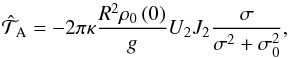$\mathrm{𝒯̂}\mathrm{A}\mathrm{=}\mathrm{-}\mathrm{2}\mathit{\pi \kappa }\frac{{\mathit{R}}^{\mathrm{2}}{\mathit{\rho }}_{\mathrm{0}}\mathrm{(}{\mathrm{0}}^{\mathrm{)}}}{\mathit{g}}{\mathit{U}}_{\mathrm{2}}{\mathit{J}}_{\mathrm{2}}\frac{\mathit{\sigma }}{{\mathit{\sigma }}^{\mathrm{2}}\mathrm{+}{\mathit{\sigma }}_{\mathrm{0}}^{\mathrm{2}}}\mathit{,}$(3)where ${\mathit{\rho }}_{\mathrm{0}}{}^{\mathrm{\right(}}\mathrm{0}^{\mathrm{\left)}}$ is the density at the ground. This function of σ is of the same form as that given by Ingersoll & Dobrovolskis (1978, Eq. (4)). The quadrupolar tidal gravitational potential and heat power are given by (P1, Eq. (74)) 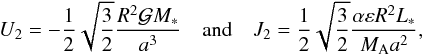$\begin{array}{c}\\ {\mathit{U}}_{\mathrm{2}}\mathrm{=}\mathrm{-}\frac{\mathrm{1}}{\mathrm{2}}\sqrt{\frac{\mathrm{3}}{\mathrm{2}}}\frac{{\mathit{R}}^{\mathrm{2}}\mathrm{𝒢}{\mathit{M}}_{\mathrm{\ast }}}{{\mathit{a}}^{\mathrm{3}}}& \mathrm{and}& {\mathit{J}}_{\mathrm{2}}\mathrm{=}\frac{\mathrm{1}}{\mathrm{2}}\sqrt{\frac{\mathrm{3}}{\mathrm{2}}}\frac{\mathit{\alpha \epsilon }{\mathit{R}}^{\mathrm{2}}{\mathit{L}}_{\mathrm{\ast }}}{{\mathit{M}}_{\mathrm{A}}{\mathit{a}}^{\mathrm{2}}}\mathit{,}\end{array}$(4)where designates the gravitational constant, ε the effective fraction of power absorbed by the atmosphere and α a shape factor depending on the spatial distribution of tidal heat sources. Denoting $\mathrm{ℱ}{}^{\mathrm{\right(}}\mathrm{\Psi }^{\mathrm{\left)}}$ the distribution of tidal heat sources as a function of the stellar zenith angle Ψ, the parameter α is defined as 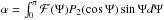$\mathit{\alpha }\mathrm{=}{{}^{\mathrm{\int }}}_{\mathrm{0}}^{\mathit{\pi }}\mathrm{ℱ}\mathrm{\left(}\mathrm{\Psi }\mathrm{\right)}{\mathit{P}}_{\mathrm{2}}\mathrm{\left(}\cos \mathrm{\Psi }\mathrm{\right)}\sin \mathrm{\Psi }\mathit{d}\mathrm{\Psi }$, where 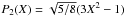${\mathit{P}}_{\mathrm{2}}\mathrm{\left(}\mathit{X}\mathrm{\right)}\mathrm{=}\sqrt{\mathrm{5}\mathit{/}\mathrm{8}}\mathrm{(}\mathrm{3}{\mathit{X}}^{\mathrm{2}}\mathrm{-}\mathrm{1}\mathrm{)}$ is the normalized Legendre polynomial of order n = 2. If we assume a heat source of the form $\mathrm{ℱ}{}^{\mathrm{\right(}}\mathrm{\Psi }^{\mathrm{\left)}}\mathrm{=}\cos \mathrm{\Psi }$ if $\mathrm{\Psi }\mathrm{\in }\mathrm{\left[}\mathrm{0}\mathit{,}\frac{\mathit{\pi }}{\mathrm{2}}\mathrm{\right]}$, and $\mathrm{ℱ}{}^{\mathrm{\right(}}\mathrm{\Psi }^{\mathrm{\left)}}\mathrm{=}\mathrm{0}$ else, we get the shape factor $\mathit{\alpha }\mathrm{=}\mathrm{1}\mathit{/}\mathrm{8}\sqrt{\mathrm{5}\mathit{/}\mathrm{2}}\mathrm{\approx }\mathrm{0.19}$. The tidal torque exerted on the atmosphere is partly transmitted to the telluric core. The efficiency of this dynamical (viscous) coupling between the two layers is weighted by a parameter β (0 ≤ β ≤ 1). Hence, with ω₀ = σ₀/ 2, the transmitted torque (Eq. (3)) becomes ${\mathrm{𝒯}}_{\mathrm{A}}\mathrm{=}\frac{\mathrm{3}}{\mathrm{32}}\frac{\mathit{\kappa \beta }{\mathit{R}}^{\mathrm{4}}\mathrm{𝒢}{\mathit{M}}_{\mathrm{\ast }}\mathit{\alpha \epsilon }{\mathit{L}}_{\mathrm{\ast }}}{{\mathrm{ℛ}}_{\mathrm{A}}{\mathit{T}}_{\mathrm{0}}\hspace{0.17em}{\mathit{a}}^{\mathrm{5}}}\frac{\mathit{\omega }}{{\mathit{\omega }}^{\mathrm{2}}\mathrm{+}{\mathit{\omega }}_{\mathrm{0}}^{\mathrm{2}}}\mathrm{·}$(5)

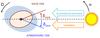Fig. 1 Tidal elongation of a Venus-like rotating planet, composed of a solid core (brown) and a gaseous atmosphere (blue), and submitted to gravitational and thermal forcings.

2.3. Solid tidal torque

For simplicity and because of the large variety of possible rheologies, we have assumed that the telluric core behaves like a damped oscillator. In this framework, called the Maxwell model, the tidal torque exerted on an homogeneous body can be expressed (e.g. Remus et al. 2012) ${\mathrm{𝒯}}_{\mathit{S}}\mathrm{=}\frac{\mathrm{3}}{\mathrm{4}}\frac{\mathrm{𝒢}{\mathit{M}}_{\mathrm{\ast }}^{\mathrm{2}}{\mathit{R}}^{\mathrm{5}}}{{\mathit{a}}^{\mathrm{6}}}\mathrm{\Im }\left\{{\mathit{k}}_{\mathrm{2}}\right\}\mathit{,}\hspace{0.17em}\mathrm{with}\mathrm{\Im }\left\{{\mathit{k}}_{\mathrm{2}}\right\}\mathrm{=}\mathrm{-}\frac{\mathrm{3}\mathit{K}}{\mathrm{2}}\frac{{\mathit{\sigma }}_{\mathrm{M}}\mathit{\sigma }}{{\mathit{\sigma }}_{\mathrm{M}}^{\mathrm{2}}\mathrm{+}{\mathrm{(}\mathrm{1}\mathrm{+}{\mathit{K}}^{\mathrm{)}}}^{\mathrm{2}}{\mathit{\sigma }}^{\mathrm{2}}}\mathit{,}$(6)the imaginary part of the second order Love number (k₂), K a non-dimensional rheological parameter, σ_M the relaxation frequency of the material composing the body, with $\mathit{K}\mathrm{=}\frac{\mathrm{38}\mathit{\pi }}{\mathrm{3}}\frac{{\mathit{R}}^{\mathrm{4}}\mathit{G}}{\mathrm{𝒢}{\mathit{M}}_{\mathrm{P}}^{\mathrm{2}}} \mathrm{and} {\mathit{\sigma }}_{\mathrm{M}}\mathrm{=}\frac{\mathit{G}}{\mathit{\eta }}\mathit{,}$(7)where G and η are the effective shear modulus and viscosity of the telluric core. Finally, introducing the frequency ω_M = σ_M/⁽2 + 2K⁾, we obtain ${\mathrm{𝒯}}_{\mathit{S}}\mathrm{=}\mathrm{-}\frac{\mathrm{9}}{\mathrm{8}}\frac{\mathrm{𝒢}{\mathit{M}}_{\mathrm{\ast }}^{\mathrm{2}}{\mathit{R}}^{\mathrm{5}}\mathit{K}{\mathit{\omega }}_{\mathrm{M}}}{\mathrm{(}\mathrm{1}\mathrm{+}{\mathit{K}}^{\mathrm{)}}{\mathit{a}}^{\mathrm{6}}}\frac{\mathit{\omega }}{{\mathit{\omega }}^{\mathrm{2}}\mathrm{+}{\mathit{\omega }}_{\mathrm{M}}^{\mathrm{2}}}\mathrm{·}$(8)

3. Rotational equilibrium states

3.1. Theory

The total torque exerted on the planet is the sum of the two previous contributions: . When the atmospheric and solid torques are of the same order of magnitude, several equilibria can exist, corresponding to (Fig. 2). The synchronization is given by Ω₀ = n and non-synchronized retrograde and prograde states of equilibrium, denoted Ω₋ and Ω₊ respectively, are expressed as functions of a (Eqs. (5) and (8)) ${\mathrm{\Omega }}_{\mathrm{-}}\mathrm{(}{\mathit{a}}^{\mathrm{)}}\mathrm{=}\mathit{n}\mathrm{-}{\mathit{\omega }}_{\mathrm{eq}}\mathrm{(}{\mathit{a}}^{\mathrm{)}} \mathrm{and} {\mathrm{\Omega }}_{\mathrm{+}}\mathrm{(}{\mathit{a}}^{\mathrm{)}}\mathrm{=}\mathit{n}\mathrm{+}{\mathit{\omega }}_{\mathrm{eq}}\mathrm{(}{\mathit{a}}^{\mathrm{)}}\mathit{,}$(9)where the difference to synchronization, ω_eq, is given by 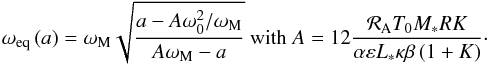${\mathit{\omega }}_{\mathrm{eq}}\mathrm{(}{\mathit{a}}^{\mathrm{)}}\mathrm{=}{\mathit{\omega }}_{\mathrm{M}}\sqrt{\frac{\mathit{a}\mathrm{-}\mathit{A}{\mathit{\omega }}_{\mathrm{0}}^{\mathrm{2}}\mathit{/}{\mathit{\omega }}_{\mathrm{M}}}{\mathit{A}{\mathit{\omega }}_{\mathrm{M}}\mathrm{-}\mathit{a}}}\mathrm{with}\mathit{A}\mathrm{=}\mathrm{12}\frac{{\mathrm{ℛ}}_{\mathrm{A}}{\mathit{T}}_{\mathrm{0}}{\mathit{M}}_{\mathrm{\ast }}\mathit{RK}}{\mathit{\alpha \epsilon }{\mathit{L}}_{\mathrm{\ast }}\mathit{\kappa \beta }\mathrm{(}\mathrm{1}\mathrm{+}{\mathit{K}}^{\mathrm{)}}}\mathrm{·}$(10)

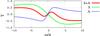Fig. 2 Normalized total tidal torque exerted on a Venus-like planet (in red) and its solid (in green) and atmospheric (in blue) components as functions of the forcing frequency ω/n with ω0/n = 2 and ωM/n = 6.

As a first approximation, we consider that parameters A, ω₀ and ω_M do not vary with the star-planet distance. In this framework, the equilibrium of synchronization is defined for all orbital radii, while those associated with Eq. (10) only exist in a zone delimited by a_inf<a<a_sup, the boundaries being ${\mathit{a}}_{\inf }\mathrm{=}\mathit{A}{\mathit{\omega }}_{\mathrm{0}}{\mathit{\lambda }}^{-1} \mathrm{and} {\mathit{a}}_{\sup }\mathrm{=}\mathit{A}{\mathit{\omega }}_{\mathrm{0}}\mathit{\lambda ,}$(11)with the ratio $\mathit{\lambda }\mathrm{=}\max {}^{\mathrm{(}}\mathit{\omega }_{\mathrm{0}}\mathit{/}{\mathit{\omega }}_{\mathrm{M}}\mathit{,}{\mathit{\omega }}_{\mathrm{M}}\mathit{/}{\mathit{\omega }}_{\mathrm{0}}{}^{\mathrm{)}}$. In the particular case where ω₀ = ω_M, the distance a_eq = Aω₀ corresponds to an orbit for which the atmospheric and solid tidal torques counterbalance each other whatever the angular velocity (Ω) of the planet. Studying the derivative of ω_eq (Eq. (10)), we note that when the star-planet distance increases, the pseudo-synchronized states of equilibrium get closer to the synchronization (ω_M<ω₀) or move away from it (ω_M>ω₀), depending on the hierarchy of frequencies associated with dissipative processes. To determine the stability of the identified equilibria, we introduce the first order variation δω such that ω = ω_eq + δω and study the sign of in the vicinity of an equilibrium position for a given a. We first treat the synchronization, for which ${\mathrm{𝒯}}_{\mathrm{S}\mathrm{+}\mathrm{A}}\hspace{0.17em}\mathrm{\propto }\hspace{0.17em}\mathrm{sign}\mathrm{(}\mathit{a}\mathrm{-}{\mathit{a}}_{\mathrm{eq}}\mathrm{)}\mathit{\delta \omega } \mathrm{with} {\mathit{a}}_{\mathrm{eq}}\mathrm{=}\mathit{A}\frac{{\mathit{\omega }}_{\mathrm{0}}^{\mathrm{2}}}{{\mathit{\omega }}_{\mathrm{M}}}\mathrm{·}$(12)We note that a_eq = a_inf if ω₀<ω_M and a_eq = a_sup otherwise. In the vicinity of non-synchronized equilibria, we have ${\mathrm{𝒯}}_{\mathrm{S}\mathrm{+}\mathrm{A}}\hspace{0.17em}\mathrm{\propto }\hspace{0.17em}{\mathit{n}}^{\mathrm{4}}{\mathit{\omega }}_{\mathrm{M}}\frac{{\mathit{\omega }}_{\mathrm{eq}}^{\mathrm{2}}\mathrm{(}{\mathit{\omega }}_{\mathrm{0}}^{\mathrm{2}}\mathrm{-}{{\mathit{\omega }}_{\mathrm{M}}^{\mathrm{2}}}^{\mathrm{)}}}{{\mathrm{(}{\mathit{\omega }}_{\mathrm{eq}}^{\mathrm{2}}\mathrm{+}{{\mathit{\omega }}_{\mathrm{M}}^{\mathrm{2}}}^{\mathrm{)}}}^{\mathrm{2}}\mathrm{(}{\mathit{\omega }}_{\mathrm{eq}}^{\mathrm{2}}\mathrm{+}{{\mathit{\omega }}_{\mathrm{0}}^{\mathrm{2}}}^{\mathrm{)}}}\mathit{\delta \omega }\mathit{.}$(13)Therefore, within the interval $\mathit{a}\mathrm{\in }{}^{\mathrm{]}}\mathit{a}_{\inf }\mathit{,}{\mathit{a}}_{\sup }{}^{\mathrm{[}}$, the stability of states of equilibrium also depends on the hierarchy of frequencies. If ω_M<ω₀ (ω_M>ω₀), he synchronized state of equilibrium is stable (unstable) and the pseudo-synchronized ones are unstable (stable). For a<a_inf the gravitational tide predominates and the equilibrium at Ω = n is stable. It becomes unstable for a>a_sup, because the torque is driven by the thermal tide.

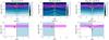Fig. 3 Top: solid (left panel), atmospheric (middle panel) and total tidal torque (right panel) exerted on a Venus-like planet as functions of the reduced forcing frequency ω/n (horizontal axis) and orbital radius a in logarithmic scale (vertical axis). The colour level corresponds to the torque in logarithmic scale with isolines at . Bottom: sign of the solid (left panel), atmospheric (middle panel) and total (right panel) tidal torque as functions of the same parameters: white (blue) areas are associated with positive (negative) torques. Stable (unstable) states of equilibrium are designated by blue (red) lines (with A = 1.88 × 1019 m s). The pink band corresponds to the habitable zone for the black body equilibrium temperature Teq = 288 K ± 20% for a 1 M⊙ Solar-type star at the age of the Sun.

3.2. Comparison with previous works

In many early studies dealing with the spin rotation of Venus, the effect of the gravitational component on the atmosphere is disregarded so that the atmospheric tide corresponds to a pure thermal tide (e.g. Dobrovolskis & Ingersoll 1980; Correia & Laskar 2001; Correia et al. 2003, 2008; Cunha et al. 2015). Moreover, the torque induced by the tidal elongation of the solid core is generally assumed to be linear in these works. This amounts to considering that |ω| ≪ ω_M and ω₀ ≪ ω_M. Hence, the relation Eq. (10) giving the positions of non-synchronized equilibria can be simplified: ${\mathit{\omega }}_{\mathrm{eq}}\mathrm{=}\sqrt{\frac{{\mathit{\omega }}_{\mathrm{M}}}{\mathit{A}}\mathit{a}\mathrm{-}{\mathit{\omega }}_{\mathrm{0}}^{\mathrm{2}}}\mathit{.}$(14)Following Correia et al. (2008), we take ω₀ = 0. We then obtain ω_eq∝$\sqrt{\mathit{a}}$ while Correia et al. (2008) found ω_eq∝a. This difference can be explained by the linear approximation of the sine of the phase lag done in this previous work. Given that the condition ω₀<ω_M is satisfied, the non-synchronized states of equilibrium are stable in this case.

By using a GCM, Leconte et al. (2015) obtained numerically for the atmospheric tidal torque an expression similar to the one given by Eq. (3). They computed with this expression the possible states of equilibrium of Venus-like planets by applying to the telluric core the Andrade and constant-Q models and showed that for both models, up to five equilibrium positions could appear. This is not the case when the Maxwell model is used, as shown by the present work. Hence, although these studies agree well on the existence of several non-synchronized states of equilibrium, they also remind us that the theoretical number and positions of these equilibria depend on the models used to compute tidal torques and more specifically on the rheology chosen for the solid part.

4. The case of Venus-like planets

We now illustrate the previous results for Venus-like planets (Table 1). The frequency ω_M is adjusted so that the present angular velocity of Venus corresponds to the retrograde state of equilibrium identified in the case where the condition ω_M>ω₀ is satisfied (Ω₋ in Eq. (9)).In Fig. 3, we plot the resulting tidal torque and its components, as well as their signs, as functions of the tidal frequency and orbital radius. These maps show that the torque varies over a very large range, particularly the solid component ( ∝a^-6 while ∝a^-5). The combination of the solid and atmospheric responses generates the non-synchronized states of equilibrium observed on the bottom left panel, which are located in the interval ${}^{\mathrm{]}}\mathit{a}_{\inf }\mathit{,}{\mathit{a}}_{\sup }{\mathrm{[}}^{}$ (see Eq. (11)) and move away from the synchronization when a increases (see Eq. (10)), as predicted analytically.

For illustration, in Fig. 4, we show the outcome of a different value of ω_M, with ω₀>ω_M, contrary to Fig. 3 where ω_M>ω₀. We observe the behaviour predicted analytically in Sect. 3. In Fig. 3, the non-synchronized equilibria are stable and move away from the synchronization when a increases, but they are unstable in Fig. 4.

We note that the value of the solid Maxwell frequency obtained for stable non-synchronized states of equilibrium, ω_M = 1.075 × 10^-4 s^-1, is far higher than those of typical solid bodies (ω_M ~ 10^-10 s^-1, see Efroimsky 2012). The Maxwell model, because of its decreasing rate as a function of ω (i.e. ∝ ω^-1), underestimates tidal torque for tidal frequencies that are greater than ω_M, which leads to overestimate the Maxwell frequency when equalizing atmospheric and solid torques. Using the Andrade model for the solid part could give more realistic values of ω_M, as proved numerically by Leconte et al. (2015), because the decreasing rate of the torque is lower in the Andrade model than in the Maxwell model (i.e. ∝ ω^{− α} with α = 0.2−0.3).

Finally, we must discuss the assumption we made when we supposed that the parameters of the system did not depend on the star-planet distance. The surface temperature of the planet and the radiative frequency actually vary with a. If we consider that T₀ is determined by the balance between the heating of the star and the black body radiation of the planet, then T₀∝a^{− 1/2}. As σ₀∝${\mathit{T}}_{\mathrm{0}}^{\mathrm{3}}$, we have σ₀∝a^{− 3/2}. These new dependences modify neither the expressions of ω_eq (Eq. (10)), nor the stability conditions of the states of equilibrium (Eqs. (12) and (13)). However, they have repercussions on the boundaries of the region where non-synchronized states exist. This changes are illustrated by Fig. 4 (bottom panel), which shows the stability diagram of Fig. 3 (bottom left panel) computed with the functions T₀(a) = T_0;♀(a/a_♀)^−1/2 and σ₀(a) = σ_0;♀(a/a_♀)^−3/2 (a_♀, T_0;♀ and σ_0;♀ being the semi-major axis of Venus and the constant temperature and radiative frequency of Table 1 respectively).

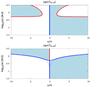Fig. 4 Sign of the total tidal torque as a function of the tidal frequency ω/n (horizontal axis) and orbital radius (a) (vertical axis) for two different cases. Top: with ω0 = 3.77 × 10-7 s-1 and ωM = 3.7 × 10-8 s-1 (ω0>ωM). Bottom: with T0 and ω0 depending on the star-planet distance and ωM>ω0. White (blue) areas correspond to positive (negative) torque. Blue (red) lines designate stable (unstable) states of equilibrium.

5. Discussion

A physical model for solid and atmospheric tides allows us to determine analytically the possible rotation equilibria of Venus-like planets and their stability. Two regimes exist depending on the hierarchy of the characteristic frequencies associated with dissipative processes (viscous friction in the solid layer and thermal radiation in the atmosphere). These dissipative mechanisms have an impact on the stability of non-synchronized equilibria, which can appear in the habitable zone since they are caused by solid and atmospheric tidal torques of comparable intensities. This study can be used to constrain the equilibrium rotation of observed super-Earths and therefore to infer the possible climates of such planets. Also here the Maxwell rheology wasused. This work can be directly applied to alternative rheologies such as the Andrade model (Efroimsky 2012). The modelling used here is based on an approach where the atmosphere is assumed to rotate uniformly with the solid part of the planet (Auclair-Desrotour et al. 2017). As general circulation is likely to play an important role in the atmospheric tidal response, we envisage examining the effect of differential rotation and corresponding zonal winds of the tidal torque in future studies.

Acknowledgments

P. Auclair-Desrotour and S. Mathis acknowledge funding by the European Research Council through ERC grant SPIRE 647383. This work was also supported by the “exoplanètes” action from Paris Observatory and by the CoRoT/Kepler and PLATO CNES grant at CEA-Saclay. A. C. M. Correia acknowledges support from CIDMA strategic project UID/MAT/04106/2013.

References

All Tables

All Figures

	Fig. 1 Tidal elongation of a Venus-like rotating planet, composed of a solid core (brown) and a gaseous atmosphere (blue), and submitted to gravitational and thermal forcings.
In the text

	Fig. 2 Normalized total tidal torque exerted on a Venus-like planet (in red) and its solid (in green) and atmospheric (in blue) components as functions of the forcing frequency ω/n with ω0/n = 2 and ωM/n = 6.
In the text

Fig. 3 Top: solid (left panel), atmospheric (middle panel) and total tidal torque (right panel) exerted on a Venus-like planet as functions of the reduced forcing frequency ω/n (horizontal axis) and orbital radius a in logarithmic scale (vertical axis). The colour level corresponds to the torque in logarithmic scale with isolines at . Bottom: sign of the solid (left panel), atmospheric (middle panel) and total (right panel) tidal torque as functions of the same parameters: white (blue) areas are associated with positive (negative) torques. Stable (unstable) states of equilibrium are designated by blue (red) lines (with A = 1.88 × 1019 m s). The pink band corresponds to the habitable zone for the black body equilibrium temperature Teq = 288 K ± 20% for a 1 M⊙ Solar-type star at the age of the Sun.

In the text

Fig. 4 Sign of the total tidal torque as a function of the tidal frequency ω/n (horizontal axis) and orbital radius (a) (vertical axis) for two different cases. Top: with ω0 = 3.77 × 10-7 s-1 and ωM = 3.7 × 10-8 s-1 (ω0>ωM). Bottom: with T0 and ω0 depending on the star-planet distance and ωM>ω0. White (blue) areas correspond to positive (negative) torque. Blue (red) lines designate stable (unstable) states of equilibrium.

In the text

References

- Auclair-Desrotour, P., Laskar, J., & Mathis, S. 2017, A&A, 603, A107 [NASA ADS] [CrossRef] [EDP Sciences] [Google Scholar]
- Chapman, S., & Lindzen, R. 1970, Atmospheric tides: Thermal and gravitational (Dordrecht: Reidel) [Google Scholar]
- Correia, A. C. M., & Laskar, J. 2001, Nature, 411, 767 [NASA ADS] [CrossRef] [PubMed] [Google Scholar]
- Correia, A. C. M., Laskar, J., & de Surgy, O. N. 2003, Icarus, 163, 1 [NASA ADS] [CrossRef] [Google Scholar]
- Correia, A. C. M., Levrard, B., & Laskar, J. 2008, A&A, 488, L63 [NASA ADS] [CrossRef] [EDP Sciences] [Google Scholar]
- Correia, A. C. M., Boué, G., Laskar, J., & Rodríguez, A. 2014, A&A, 571, A50 [NASA ADS] [CrossRef] [EDP Sciences] [Google Scholar]
- Cunha, D., Correia, A. C., & Laskar, J. 2015, Int. J. Astrobiol., 14, 233 [CrossRef] [Google Scholar]
- Demory, B.-O., Gillon, M., Madhusudhan, N., & Queloz, D. 2016, MNRAS, 455, 2018 [NASA ADS] [CrossRef] [Google Scholar]
- Dobrovolskis, A. R., & Ingersoll, A. P. 1980, Icarus, 41, 1 [NASA ADS] [CrossRef] [Google Scholar]
- Efroimsky, M. 2012, ApJ, 746, 150 [NASA ADS] [CrossRef] [Google Scholar]
- Forget, F., & Leconte, J. 2014, Phil. Trans. R. Soc. Lond. Ser. A, 372, 20130084 [Google Scholar]
- Gold, T., & Soter, S. 1969, Icarus, 11, 356 [NASA ADS] [CrossRef] [Google Scholar]
- Ingersoll, A. P., & Dobrovolskis, A. R. 1978, Nature, 275, 37 [NASA ADS] [CrossRef] [Google Scholar]
- Kasting, J. F., Whitmire, D. P., & Reynolds, R. T. 1993, Icarus, 101, 108 [NASA ADS] [CrossRef] [PubMed] [Google Scholar]
- Kaula, W. M. 1964, Reviews of Geophysics and Space Physics, 2, 661 [NASA ADS] [CrossRef] [Google Scholar]
- Kopparapu, R. K., Ramirez, R. M., SchottelKotte, J., et al. 2014, ApJ, 787, L29 [Google Scholar]
- Leconte, J., Wu, H., Menou, K., & Murray, N. 2015, Science, 347, 632 [NASA ADS] [CrossRef] [Google Scholar]
- Marov, M. Y., Avduevskij, V. S., Kerzhanovich, V. V., et al. 1973, J. Atmos. Sci., 30, 1210 [NASA ADS] [CrossRef] [Google Scholar]
- Mayor, M., & Queloz, D. 1995, Nature, 378, 355 [Google Scholar]
- Mohr, P. J., Taylor, B. N., & Newell, D. B. 2012, J. Phys. Chem. Ref. Data, 41, 043109 [NASA ADS] [CrossRef] [Google Scholar]
- Pollack, J. B., & Young, R. 1975, J. Atmos. Sci., 32, 1025 [NASA ADS] [CrossRef] [Google Scholar]
- Remus, F., Mathis, S., Zahn, J.-P., & Lainey, V. 2012, A&A, 541, A165 [NASA ADS] [CrossRef] [EDP Sciences] [Google Scholar]
- Seiff, A., Kirk, D. B., Young, R. E., et al. 1980, J. Geophys. Res., 85, 7903 [Google Scholar]
- Shen, M., & Zhang, C. Z. 1990, Icarus, 85, 129 [NASA ADS] [CrossRef] [Google Scholar]