| Issue |
A&A
Volume 601, May 2017
|
|
|---|---|---|
| Article Number | A51 | |
| Number of page(s) | 8 | |
| Section | The Sun | |
| DOI | https://doi.org/10.1051/0004-6361/201629871 | |
| Published online | 27 April 2017 | |
Hemispheric progression of solar cycles in solar magnetic field data and its relation to the solar dynamo models
1 Leibniz-Institut für Astrophysik Potsdam, An der Sternwarte 16, 14482 Potsdam, Germany
e-mail: This email address is being protected from spambots. You need JavaScript enabled to view it.
2 Geneva Observatory, University of Geneva, Geneva, Switzerland
e-mail: This email address is being protected from spambots. You need JavaScript enabled to view it.
3 Department of Geoscience, Aarhus University, Høegh-Guldbergs Gade 2, 8000 Aarhus C, Denmark
4 Stellar Astrophysics Centre, Department of Physics and Astronomy, Aarhus University, Ny Munkegade 120, 8000 Aarhus C, Denmark
Received: 10 October 2016
Accepted: 3 March 2017
Abstract
Aims. We aim to characterise the solar cycle progression simultaneously at different latitudes in each solar hemisphere using solar magnetic field data provided by the Wilcox Solar Observatory (WSO). We also investigate whether the features observed in the WSO data are best explained by the Babcock-Leighton (BL) mechanism and/or turbulent helicity as the α-effect in solar dynamos.
Methods. We analysed the hemispheric solar-cycle progression of the Sun’s magnetic field in different 15° latitudinal bands, which allow us to explore the extent of cycle overlap. We also investigated the Waldmeier Rule, and the relationship between decay rates and peak amplitudes of the same cycle. These aspects of the solar-cycle progression can be explained in different ways by solar dynamo models depending on the source of the α-effect.
Results. The progression of the last four solar cycles in different latitudinal bands reveals that the degree of overlap between consecutive cycles is small and is more likely to be confined to low solar latitudes. We also found that the southern and northern solar hemispheres behave differently for the last four solar cycles, suggesting a slight decoupling between the hemispheres. The results also reveal a strong correlation between the decay rates and the peak amplitudes of the solar cycles.
Key words: Sun: activity / Sun: magnetic fields / Sun: general / dynamo
© ESO, 2017
1. Introduction
The observed cyclic evolution of solar magnetic features at and above the photosphere is believed to be driven by the dynamo operating inside the Sun. Two basic processes are involved in exciting a self-sustainable dynamo: the Ω- and α-effects. The shearing of any poloidal field by the differential rotation can generate the toroidal part of the magnetic field. This is the so-called Ω-effect, on which a clear consensus is reached. Conversely, various mechanisms have been suggested concerning the re-generation of a poloidal field from a toroidal field. Two of the most promising mechanisms are (i) the Babcock-Leighton (BL) mechanism (Babcock 1961; Leighton 1964, 1969), and (ii) the effect of rotating turbulence, where helical twisting of the toroidal field lines by the Coriolis force generates a poloidal field, known as turbulent helicity (Parker 1955a,b; Steenbeck & Krause 1969).
In the BL mechanism, diffusion and transportation of tilted bipolar active regions by the surface meridional flow and supergranular diffusion act as poloidal magnetic field sources at the solar surface (Babcock 1961; Leighton 1964; Wang et al. 1989; Wang & Sheeley 1991). The poleward meridional flow brings the poloidal field sources to the poles and in turn causes the polarity reversal at sunspot maximum (Cameron & Schüssler 2015). The meridional flow then penetrates below the base of the convection zone and is responsible for the generation and equatorward propagation of the bipolar activity structures at low latitudes at the solar surface (Dikpati & Charbonneau 1999; Nandy & Choudhuri 2001, 2002; Hathaway et al. 2003). The inclusion of a poleward surface meridional flow along with an equatorward subsurface meridional flow has led to the development of the so-called flux transport (FT) dynamo models (Wang et al. 1991; Dikpati & Charbonneau 1999; Nandy & Choudhuri 2001). There are several types of FT dynamo models, which produce the α-effect either as a pure BL-mechanism or a pure α-turbulent effect operating in the tachocline, or, alternatively, in the whole convection zone. More recently, dynamo models operating with α-turbulence and BL-mechanisms simultaneously as poloidal field sources have also emerged (Dikpati & Gilman 2001; Passos et al. 2014; Belucz & Dikpati 2013).
We note that within the αΩ turbulent dynamos, equatorward propagation of the sunspots are driven by dynamo waves. But the α and Ω mechanisms can be located either at the core-envelope interface, throughout the solar convection zone, or in the subsurface layers (see reviews by Brandenburg & Subramanian 2005; Charbonneau 2010, 2014). This has some important implications. In fact, due to a change in the sign of the rotation profile in the tachocline (Ruediger & Brandenburg 1995), a thin shell αΩ dynamo wave can generate both poleward and equatorward migration of solar magnetic activity (Parker 1993; Charbonneau & MacGregor 1997). In contrast, a distributed or subsurface dynamo can only generate a poleward or an equatorward migration of magnetic activity.
Several observational features in the sunspot butterfly diagram, such as the confinement of the sunspot generation to latitudinal activity bands within 30° of the solar equator, equatorward sunspot migration, slowing down of the drift velocity of sunspots towards the solar equator, and the delay of the onset of a forthcoming cycle (Maunder 1904), which results in succeeding solar cycles overlapping by two to three years (Harvey 1992), can be explained by the solar dynamo models depending on where the Ω-and α-effects are located and whether the dynamo is governed by FT or dynamo-wave processes.
Together with the features observed in the solar butterfly diagram, there are also empirical relationships found in the sunspot records, such as the linear anti-correlation between the time interval from the minimum to the succeeding peak amplitude of a solar cycle (hereafter denoted peak time of a solar cycle) and the same cycle’s peak amplitude, known as the Waldmeier Rule (Waldmeier 1935). The physical mechanisms underlying these empirical relationships can also be explained by solar dynamo models. The αΩ-dynamos generate solar-cycle patterns that are in accordance with the Waldmeier effect, where the higher peak amplitudes are reached after shorter peak times (Hoyng 1993; Ossendrijver & Hoyng 1996; Ossendrijver et al. 1996; Pipin et al. 2012). On the other hand, BL dynamos can generate both positive and negative correlations between the peak amplitude and peak times of the solar cycles, depending on whether the random noise is applied to the meridional circulation or the poloidal source term, which generates a significant spread in cycle periods, in either high-or low-diffusivity regimes (Charbonneau & Dikpati 2000; Karak & Choudhuri 2011). Furthermore dynamo models tend to limit the dynamo action to a 0−45° band on either side of the solar equator (Nandy & Choudhuri 2002; Nandy 2004).
In this study, we have used magnetic field data provided by the Wilcox Solar Observatory (WSO; Scherrer et al. 1977; Hoeksema et al. 2010), because the results from mean-field dynamo model simulations are generally represented as the magnetic field energy and/or strength. To investigate the properties of the solar cycle progression as a function of latitude and compare them to the results from various solar dynamo models, we used the WSO magnetic field data. For this purpose, we measured the degree of overlap between consecutive solar cycles at the time of activity minimum and investigate if the evolution of magnetic activity follows the Waldmeier Rule, as different assumptions on alpha mechanisms in solar dynamos lead to different features in temporal and spatial evolution of solar activity.
2. The magnetic field data
To identify the features in the solar cycle progression of magnetic field data, we used synoptic photospheric magnetic field maps of the radial magnetic field (Br) obtained from line-of-sight magnetogram observations by the WSO. The synoptic charts of the solar magnetic field are assembled from individual magnetograms observed over the course of a Carrington rotation (CR). These maps contain the most relevant information about the temporal and spatial distribution of the large-scale magnetic field over the solar surface.
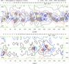 |
Fig. 1 Contour maps show the distribution of magnetic flux over the photosphere during the maximum of solar cycle 24 (top panel) and the minimum of solar cycle 23 (bottom panel). The field above 70°s is not resolved. Blue, light shading shows the positive regions, while red shading indicates negative regions. The neutral line is black. Contours are indicated. Inverted carets show times of contributing magnetograms (taken from the WSO webpage). |
The surface magnetic field distributions at two different epochs of solar activity, the maximum of solar cycle 24 and the minimum phase of solar cycle 23, are shown in the top and the bottom panels of Fig. 1, respectively. Near the maximum of solar cycle 24 (top panel of Fig. 1), the magnetic field spreads over a wider range of latitudes between 0° ≤ θ ≤ 30°, compared to the minimum phase of solar cycle 23 (bottom panel of Fig. 1), where the activity is confined to latitudes below 15°. In addition, no magnetic activity is observed above 30° in both solar hemispheres during the maximum of solar cycle 24, while during the minimum phase of solar cycle 23, magnetic fields are observed in the northern solar hemisphere, but the polarity is reversed compared to the ones in the southern solar hemisphere.
During the dates between 21−26 December 1996 around the solar equatorial region (bottom panel of Fig. 1), we observed bipolar active regions, where the leading polarity is positive (the blue contour lines). However, towards 4−5 January 1997 at around 30° in the southern solar hemisphere, the newly emerging bipolar activity region exhibits an opposite polarity structure, where the leading polarity is negative (red contour lines). This polarity is in phase with the poloidal field polarity above 60° latitude, implying that these bipolar active regions belong to the new cycle as they have the right leading polarity. This feature can be identified as the overlap of two successive solar cycles, meaning that there are still bipolar active regions at low solar latitudes that belong to the previous solar cycle, while new bipolar active regions of the new solar cycle have started to emerge at higher latitudes.
The WSO data used in this study span the time period 1976–2016, starting with CR 1642 (27 May 1976), and ending with CR 2182 (23 September 2016). For each map per CR, we carried out spherical harmonic analysis of the WSO data using the Legendre-transform software provided by the potential field source surface (PFSS) package of SolarSoft following the recipe given in DeRosa et al. (2012). As a result, we obtained time series of complex coefficients  for a series of modes spanning the spherical harmonic degrees ℓ = 1,...,60. The complex coefficients are proportional to the amplitude of each spherical harmonic mode
  for spherical harmonic degree ℓ and azimuthal order m (DeRosa et al. 2012), so that
 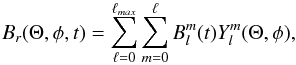 (1)where Θ, φ, and t denote colatitude, longitude, and, time, respectively. The energies in each (ℓ, m) mode are calculated by squaring the coefficients,
  .
.
3. Analyses and results
3.1. Degradation at higher ℓ
To obtain the energy spectra of the WSO data, we average the energies for each spherical harmonic degree “ℓ” both over time and order “m” (Fig. 2). The mean energy calculated for each spherical harmonic degree ℓ shows a sharp decrease around ℓ = 15 (Fig. 2). This implies that the WSO magnetograph does not adequately resolve the modes higher than ℓ = 15, resulting from the low spatial resolution of the WSO magnetograph (DeRosa et al. 2012). Therefore, we limit our further analyses to the spherical harmonic degrees spanning ℓ = 1,...,15.
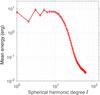 |
Fig. 2 Time-averaged energies in each spherical harmonic modes ℓ. |
3.2. Temporal evolution of the Sun’s large-scale magnetic field
To calculate the surface total magnetic energy of the Sun, we summed the total energies over the spherical harmonic degrees 1 ≤ ℓ ≤ 15 and −ℓ ≤ m ≤ + ℓ, which is identified as the Sun’s large-scale magnetic field in this study. We then smoothed the data using 2 × 11-point moving average window to get rid of high-frequency variations in the data set. The 99% confidence intervals of the mean is calculated using the equation given as 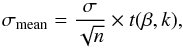 (2)for the data included in the window of the moving average. In the above equation, σmean denotes the confidence interval of the mean, while σ is the standard deviation of the data of length “n”. The multiplier t(β,k) shows the critical t-value for significance level β, which is 0.01 in this study, and for the degree of freedom k, which equals to n−1 (see Woodbury 2002, for details).
The temporal evolution of the total energy in the large-scale magnetic field of the Sun is shown in Fig. 3a. The total magnetic energy obtained for the full disc exhibits double-peak structures during solar cycles 22 and 23. Superposition of slightly out-of phase hemispheric sunspot activity (Durrant & Wilson 2003), and slightly decoupled solar hemispheres (Temmer et al. 2006) are among the proposed mechanisms that causes the observed double-peak structures. To investigate whether this behaviour caused by the out-of-phase progression of the activity in the southern and northern solar hemispheres, as previously proposed by Durrant & Wilson (2003), we calculated the total magnetic energies for the two solar hemispheres. This was done by first simply zeroing out the magnetic fields measured in each hemisphere, respectively, and then re-calculate the energies again using the PFSS package of SolarSoft. The total energies for the northern and southern solar hemispheres are presented in Figs. 3b and c, respectively. The presence of the double-peak structures, especially in the southern solar hemisphere, indicates that the observed feature does not stem from the out-of-phase progression of the activity in the two hemispheres. A decreasing trend can be seen in the Sun’s large-scale magnetic field starting towards the end of solar cycle 22 (≈1995) and still continuing over solar cycle 24 (Fig. 3a). A similar decreasing trend can also be observed in the energy in both hemispheres, where it is more pronounced in the northern solar hemisphere. Additionally, although the total magnetic energy levels are similar in the two hemispheres, they show distinct differences during the solar cycle maxima, which may indicate that the two hemispheres are to some extent decoupled (Figs. 3b and c).
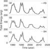 |
Fig. 3 Temporal evolution of the Sun’s large scale magnetic field as characterized by a) the total magnetic energy observed on the full disc (FD), b) the total energy in the northern solar hemisphere (NH), and c) the southern solar hemisphere (SH). The shaded areas show 99% confidence intervals (see text). |
3.3. Progression of solar activity at different latitudes
We aim to characterise and compare the properties observed during the progression of solar magnetic activity cycles to investigate, (i) similarities and differences in the rise and decay time at different latitudes, (ii) the duration and extent of the degree of overlap between succeeding cycles, since these features may be directly related to the meridional circulation speed throughout a solar cycle. To achieve these aims, we calculated the total magnetic energies in 15° latitudinal intervals extending from 45° S to 45° N solar hemispheres with the same method we used to calculate the hemispherical total magnetic energies (see Sect. 3.2). The reason for choosing this specific range is based on the sunspot observations that show the progression of a solar cycle is characterised by emerging magnetic activity regions at ≈40° latitude at the onset of a solar cycle, and propagation of these active regions towards the equator. The sunspot activity reaches its maximum at ≈15° latitude and ends at ≈8° latitude. Using the energies in selected latitudinal bands, we tracked this behaviour in an attempt to identify details in the solar activity propagation.
Rise time is defined as the period between a minimum and one year before the peak time of the succeeding cycle, and if the maximum of a cycle exhibits multiple peaks, then the rise time is defined as the period between cycle minimum and one year before the first peak of the succeeding cycle. The amplitudes observed one year before the first peak is defined as the rise peaks. The decay rate is calculated following Hazra et al. (2015), which is defined as the slope between the magnetic energy difference between a year after the peak time and a year before the following minimum. If a cycle shows multiple peaks, then the decay rate is defined as the slope between the magnetic energy difference between one year after the last peak and one year before the following minimum. These definitions are made based on the fact that the solar cycle maximum is identified as a phase, rather than a peak moment in this study. In the flux transport dynamo models the rise and decay times are governed by the meridional flow, which is found to vary over a solar cycle, that is, faster (slower) during the minimum (maximum) phase (González Hernández et al. 2008).
To identify the multiple peaks during a solar cycle, we followed the method of Norton & Gallagher (2010). In this method, the authors are determined by first choosing the maximum value in each solar cycle and then finding the secondary maxima with values at least 50% of the primary peak (see Norton & Gallagher 2010, for details).
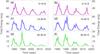 |
Fig. 4 Smoothed total magnetic energy calculated for 0–15, 15–30, and 30–45 degree latitudinal bands in northern (left panels) and southern (right panels) hemispheres, and the shades show 99% errors. |
Cyclic magnetic activity characterises all ranges of latitudes under consideration (Fig. 4). This is also observed in helioseismic observations, where the acoustic mode of oscillations were decomposed into spherical harmonics (Simoniello et al. 2013, 2016). The total energies in each latitudinal band show variations in phase with the sunspot numbers, attaining their maximum (minimum) energies during sunspot maximum (minimum). An interesting feature observed over the maxima of solar-activity cycles at different latitudes is the timing of the highest peak (Fig. 4). The solar-cycle maximum is observed at the second peaks during solar cycles 22, 23, and 24 in 15–30° S latitudinal band, while it is always the first peak in the 15–30° N for solar cycles 23 and 24. The activity is highest during the first peaks of solar cycles 22, 23, and 24 in the 30–45° S band, while in the northern solar hemisphere for the same latitudinal band there is only one peak for the last four solar cycles (Fig. 4).
3.4. Delay of the onsets of solar cycles at different latitudes
We tabulate the cycle length and the minimum times between the succeeding solar cycles for each latitudinal band to investigate the cycle-wise delay of the onsets of solar cycles (Table 1). When the cycle onsets at latitudes 0–15° N (S) are compared to the onsets at 30–45° N (S), where the sunspot formation generally takes place at the onset of a solar cycle, we observe that the onsets of the solar cycles at the 0–15° N (S) band are always delayed (Table 1). Furthermore, this delay does not always result in longer cycle lengths at latitudes below 15° N and S compared to higher latitudes, and the cycle lengths at each latitude are always comparable.
Minima, maxima and cycle lengths of the energies observed in the latitudinal energy bands in both hemispheres.
To quantify the delay time between changes in the 0–15° north and south bands and the other latitudinal bands, we perform cross-correlation analyses. The results show that a new cycle first begins in the 30–45° N around 22 CRs before the cycle begins in the 0−15° N band (Table 2). Further, the delay between the 30–45° N and the 15–30° N bands is 10 CRs. The southern solar hemisphere also shows a similar behaviour where the cycle starts at 30–45° S around 19 CRs before the cycle begins in the 0–15° S, while the delay between the 30–45° S and the 15–30° S bands is 6 CRs (Table 2).
Cross-correlation coefficients calculated between the energy in 0–15° N versus the other latitudinal bands in the northern hemisphere, and 0–15° S versus the other latitudinal bands in the southern hemisphere, separately.
3.5. Latitudinal dependence of the Waldmeier rule
We also investigated whether the magnetic energy in each latitudinal band obeys the Waldmeier Rule (Waldmeier 1935), within the sunspot activity band.
In this study, we carried out a latitudinal dependency analysis over four solar cycles. We can therefore investigate the Waldmeier rule in two different ways: (i) if the Waldmeier rule applies to energies over the last four solar cycles in each latitudinal band; and (ii) if the peak times are shorter at latitudes, where the magnetic energy is stronger for each solar cycle.
The peak magnetic energies for each latitudinal band exhibit an anti-correlation with the peak times over the four observed solar cycles (solid lines in Fig. 5). Similarly, the rise times and rise amplitudes above 15° in the both hemispheres show an anti-correlation, whereas there is a positive correlation for the 0−15° N and S latitudes (dashed lines in Fig. 5).
To quantify the observed correlations in Fig. 5, we calculated the linear correlation coefficients between the peak amplitudes and peak times as well as the rise amplitudes and rise times of the cycles. We note that when the sample size is small, the sample correlation coefficient is a biased estimator of the population correlation. In this study, we use the WSO data, which covers the last four solar cycles, and we analyse six latitudinal bands implying that our sample size is small. Therefore, in order to calculate the approximately unbiased correlation coefficients in this study, we used the following equation given by Fisher (1915); ![Mathematical equation: \begin{equation} \rho=r\left [1+\frac{(1-r^{2})}{2n}\right ] , \end{equation}](/articles/aa/full_html/2017/05/aa29871-16/aa29871-16-eq34.png) (3)where ρ is the approximately unbiased correlation coefficient, r and n represent biased correlation coefficient and sample size, respectively.
(3)where ρ is the approximately unbiased correlation coefficient, r and n represent biased correlation coefficient and sample size, respectively.
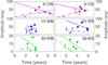 |
Fig. 5 Solar cycle peak amplitudes as a function of peak times (filled circles and solid lines) and rise amplitudes as a function of rise times (crosses and dashes lines) for each latitudinal band in the northern (left panels) and the southern (right panels) hemispheres. The bars show the 99% confidence intervals. The colour coding for each latitudinal band is the same as Fig. 4. |
Adjusted correlation coefficients between the peak times and peak amplitudes (ρWald), and between rise times and rise amplitudes (ρRR) for each latitudinal band for the northern and the southern hemispheres.
The correlation analyses following the bias correction show that the Waldmeier Rule for the peak times and peak amplitudes generally applies to the magnetic energies in each latitudinal band (Table 3), although with some modifications. Interestingly, the correlation coefficients calculated for the two hemispheres do not show a symmetrical behaviour for the Waldmeier Rule, for example the strongest anti-correlation is observed for the 0−15° N band, while it is the weakest in the same band in the southern solar hemisphere. The weakest anti-correlation in the northern hemisphere is found to be in the 15–30° band, whereas the same latitudinal band in the southern hemisphere shows the strongest anti-correlation. Similar anti-symmetric behaviour can also be observed for the relationship between the rise times and rise amplitudes to some degree. The weakest anti-correlation in the northern solar hemisphere is observed in the 30–45° band, while the same latitudinal band in the southern solar hemisphere shows the strongest anti-correlation. Further, the strongest anti-correlation in the northern solar hemisphere is at 15–30° band, while the southern solar hemisphere shows the weakest anti-correlation for the same band. The only symmetrical behaviour for the correlations between rise time and rise amplitudes are observed in 0–15° bands in each hemisphere (Table 3). These results show that the northern and southern solar hemispheres behave differently over the course of the last four solar cycles, which might suggest that they are to some extend decoupled.
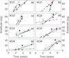 |
Fig. 6 Solar cycle peak amplitudes as a function of peak times (dots and solid lines) and rise amplitudes as a function of rise times (crosses and dashes lines) for each latitudinal band in the northern (left panels) and the southern (right panels) hemispheres for each solar cycle. The bars show the 99% confidence intervas. The colour coding for each latitudinal bands is the same with Fig. 4. |
Adjusted correlation coefficients between the peak times and peak amplitudes (ρWaldCyc), and rise times and rise amplitudes (ρRRCyc) observed for each solar cycle for the northern and southern hemispheres, respectively.
We also investigated whether the Waldmeier Rule applies to the peak magnetic energies and peak times over the same cycle but for different latitudes (the solid lines in Fig. 6). We found that there is a positive correlation between the peak amplitudes and peak times observed in each latitudinal bands (Table 4). The strongest correlations are observed for solar cycles 21 and 22 for the northern and southern solar hemispheres, respectively. The relationship between the rise times and the rise amplitudes (the dashed lines in Fig. 6) is similar to those obtained for the peak times and peak amplitudes. The strongest positive correlations between the rise times and rise amplitudes are calculated for solar cycle 21 in both hemispheres (Table 4).
We investigated whether there is a systematic relationship between the decay rates and the peak amplitudes of the same cycle (Fig. 7), as suggested by other solar activity indices, such as sunspot numbers, sunspot areas, and the solar 10.7 cm radio flux (Cameron & Schüssler 2008; Hazra et al. 2015). The relationship between the decay rates and rise amplitudes was also calculated. The results show that the decay rate is strongly correlated with the peak and rise amplitudes in the latitudinal bands under consideration. One exception to the strong positive correlations is the negative correlation between the decay rate and rise amplitude in the 0–15° N band (Table 5).
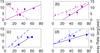 |
Fig. 7 Solar cycle decay rates observed in each latitudinal band as a function of peak amplitudes (solid lines and filled circles) and rise amplitudes (dashed lines and crosses) for each solar cycle in the northern (left panels) and the southern (right panels) hemispheres. The bars show the 99% errors. The colour coding for each latitudinal bands is the same with Fig. 4. |
Adjusted correlation coefficients between the decay rate and peak amplitude (ρDP), and decay rate and rise amplitude (ρDR) for each latitudinal band in the northern and southern hemispheres.
4. Discussion and conclusion
The progression of the Sun’s large-scale magnetic energy at different latitudes during the last four solar cycles reveals that the degree of overlap between the successive solar cycles is confined to low latitudes (≤ 15°) and it occurs only over the minimum phase. Further, the cross-correlation analysis shows that a new solar cycle starts in the 30–45° bandsaround 22 and 19 CRs before it appears in the 0–15° N and S bands, respectively (Table 2). The observed features can be explained by the BL-flux transport dynamos with or without an α-turbulence effect in the whole convection zone, which tend to result in overlaps at low latitudes, particularly during the minimum phase (Chatterjee et al. 2004). They can also be explained by dynamos with subsurface shear and turbulent kinetic helicity acting as the α-effect, which generates shorter overlapping between the two successive solar cycles by increasing the anisotropy in turbulent magnetic diffusion (Pipin & Kosovichev 2014).
This study shows that the Waldmeier rule also applies to the surface magnetic energies as it does for different solar activity proxies, such as the Wolf sunspot numbers, the group sunspot numbers, the sunspot areas and the solar 10.7 cm radio flux, (Cameron & Schüssler 2008; Dikpati et al. 2008; Hazra et al. 2015). The anti-correlation between the peak times and peak amplitudes observed in this study is stronger in the latitudinal band of 0–15° N and 15–30° S, while the 15–30° N and 0–15° S bands show weaker anti-correlations (Table 3). While the solar dynamo models that use the turbulent helicity as the α-effect source naturally generate surface features that obey the Waldmeier Rule (Hoyng 1993; Ossendrijver & Hoyng 1996; Ossendrijver et al. 1996; Pipin et al. 2012), it has recently been shown that the BL-dynamos also generate a negative relationship between the peak amplitudes and the peak times when high diffusivity is adopted in the dynamo model and random noise is introduced in the meridional flow speed (Karak & Choudhuri 2011; Hazra et al. 2015).
The double-peak structure observed for the different latitudes in the two hemispheres with different amplitudes suggests that the observed double-peak structures do not stem from averaging the magnetic energies in the northern and southern solar hemispheres, but they represent observed phenomena in separate latitudinal bands in each hemisphere, which must be caused by a physical mechanism, supporting the findings of Norton & Gallagher (2010), Georgieva (2011). Together with the results from the Waldmeier Rule, which show the solar hemispheres behave differently at different latitudinal bands, the results indicate that the two hemispheres might be decoupled to some degree (Temmer et al. 2006; Li et al. 2009; Norton & Gallagher 2010).
The observed relationship between rise times and rise amplitudes (dashed lines in Fig. 5) implies that at the latitudes between 0–15° N and S, longer rise times correspond to higher cycle-rise amplitudes. In BL-dynamo models, the meridional flow speed close to the solar equator is slower than it is at the higher latitudes meaning that the differential rotation will have more time to generate stronger toroidal fields (Karak & Choudhuri 2011; Hazra et al. 2015). Additionally, the activity bands of opposite polarity on either side of the solar equator will propagate slower due to the slow meridional flow and, in turn, will have more time to build up the magnetic energy, since cancelation of the opposite polarities by crossing of the magnetic flux over the equator proposed to occur after the cycle peak (Cameron & Schüssler 2008; Norton & Gallagher 2010; McIntosh et al. 2014). The interaction between these activity bands can also explain the observed double-peak structures (McIntosh et al. 2015). Above 15° in both hemispheres the correlations become negative, where it is weakest in 15–30° S band.
When we group the peak amplitudes and peak times in each latitudinal band for each solar cycle, we find a clear positive correlation for each solar cycle. The same feature can also be seen for the rise amplitudes and rise times (Table 4).
The correlation between the decay rates and the peak amplitudes found in this study is in agreement with previous studies, based on the Wolf sunspot number, the sunspot areas, and the 10.7 cm radio flux (Cameron & Schüssler 2008; Hazra et al. 2015). The correlations found in this study are higher than those found in Cameron & Schüssler (2008), and at the same level with those found for early phases in Hazra et al. (2015). A similar asymmetric behaviour of the northern and southern solar hemispheres as observed for the Waldmeier Rule and the anti-correlation between the rise times and rise amplitudes, is also present for the relationship between the decay rates and the peak amplitudes. This behaviour, however, is less pronounced. The correlations between the decay rate and the rise amplitudes are similar to those calculated for the decay rates and peak amplitudes, except from the 0–15° N band, which shows an anti-correlation instead. The results indicate that the decay rate of a solar cycle is strongly coupled with its rise amplitudes, even before the cycle has reached its maximum.
We must emphasize that the results obtained from the correlation analyses between rise times and rise amplitudes, peak time and peak amplitudes, and decay time and decay amplitudes are based on very restricted sample sizes. This implies that although the bias corrections were applied to the results, these results can vary when data from the future cycles are added.
In this study, we investigate the temporal evolution of hemispheric solar magnetic field energies during the last four solar cycles in different latitudinal bands using the WSO data and explain the observed features with the BL-effect and turbulent helicity, which may operate as the α-effect in solar dynamos. However, the results obtained from the WSO data provide neither strong constraints on, nor lines of evidence in favour of either of the two main mechanisms that generate a poloidal field from a pre-existing toroidal field. We conclude that providing constraints on dynamo models requires a multi-data approach over longer timescales that will cover the spatial extend from the subsurface layers of the Sun to the corona.
Acknowledgments
F.I. is grateful to the Carlsberg Foundation (CF15-0648). Funding for the Stellar Astrophysics Centre is provided by the Danish National Research Foundation (grant agreement No. DNRF106). The project has been supported by the Villum Foundation.
References
- Babcock, H. W. 1961, ApJ, 133, 572 [Google Scholar]
- Belucz, B., & Dikpati, M. 2013, ApJ, 779, 4 [NASA ADS] [CrossRef] [Google Scholar]
- Brandenburg, A., & Subramanian, K. 2005, Phys. Rep., 417, 1 [NASA ADS] [CrossRef] [Google Scholar]
- Cameron, R., & Schüssler, M. 2007, ApJ, 659, 801 [NASA ADS] [CrossRef] [Google Scholar]
- Cameron, R., & Schüssler, M. 2008, ApJ, 685, 1291 [NASA ADS] [CrossRef] [Google Scholar]
- Cameron, R., & Schüssler, M. 2015, Science, 347, 1333 [NASA ADS] [CrossRef] [Google Scholar]
- Charbonneau, P. 2010, Liv. Rev. Sol. Phys., 7, 3 [Google Scholar]
- Charbonneau, P. 2014, ARA&A, 52, 251 [Google Scholar]
- Charbonneau, P., & Dikpati, M. 2000, ApJ, 543, 1027 [NASA ADS] [CrossRef] [Google Scholar]
- Charbonneau, P., & MacGregor, K. B. 1997, ApJ, 486, 502 [NASA ADS] [CrossRef] [Google Scholar]
- Chatterjee, P., Nandy, D., & Choudhuri, A. R. 2004, A&A, 427, 1019 [NASA ADS] [CrossRef] [EDP Sciences] [Google Scholar]
- Choudhuri, A. R. 2013, in Solar and Astrophysical Dynamos and Magnetic Activity, IAU Symp., 294, 37 [NASA ADS] [Google Scholar]
- DeRosa, M. L., Brun, A. S., & Hoeksema, J. T. 2012, ApJ, 757, 96 [Google Scholar]
- Dikpati, M., & Charbonneau, P. 1999, ApJ, 518, 508 [NASA ADS] [CrossRef] [Google Scholar]
- Dikpati, M., & Gilman, P. A. 2001, ApJ, 559, 428 [NASA ADS] [CrossRef] [Google Scholar]
- Dikpati, M., Gilman, P. A., & de Toma, G. 2008, ApJ, 673, L99 [NASA ADS] [CrossRef] [Google Scholar]
- Durrant, C. J., & Wilson, P. R. 2003, Sol. Phys., 214, 23 [NASA ADS] [CrossRef] [Google Scholar]
- Fisher, R. A. 1915, Biometrica, 10, 507 [Google Scholar]
- Fletcher, S. T., Broomhall, A.-M., Salabert, D., et al. 2010, ApJ, 718, L19 [NASA ADS] [CrossRef] [Google Scholar]
- Georgieva, K. 2011, ISRN Astronomy and Astrophysics, 2011, 437838 [Google Scholar]
- González Hernández, I., Kholikov, S., Hill, F., Howe, R., & Komm, R. 2008, Sol. Phys., 252, 235 [NASA ADS] [CrossRef] [Google Scholar]
- Harvey, K. L. 1992, in The Solar Cycle, ASP Conf. Ser., 27, 335 [NASA ADS] [Google Scholar]
- Hathaway, D. H., Nandy, D., Wilson, R. M., & Reichmann, E. J. 2003, ApJ, 589, 665. [NASA ADS] [CrossRef] [Google Scholar]
- Hazra, G., Karak, B. B., Banerjee, D., & Choudhuri, A. R. 2015, Sol. Phys., 290, 1851 [NASA ADS] [CrossRef] [Google Scholar]
- Hoeksema, J. T. 2010, in Solar and Stellar Variability: Impact on Earth and Planets, Proc. of IAU Symp., 264, 222 [NASA ADS] [Google Scholar]
- Howe, R., Hill, F., Komm, R., et al. 2011, J. Phys. Conf. Ser., 271, 012074 [NASA ADS] [CrossRef] [Google Scholar]
- Howe, R., Christensen-Dalsgaard, J., Hill, F., et al. 2013, ApJ, 767, L20 [NASA ADS] [CrossRef] [Google Scholar]
- Hoyng, P. 1993, A&A, 272, 321 [NASA ADS] [Google Scholar]
- Karak, B. B., & Choudhuri, A. R. 2011, MNRAS, 410, 1503 [NASA ADS] [Google Scholar]
- Leighton, R. B. 1964, ApJ, 140, 1547 [Google Scholar]
- Leighton, R. B. 1969, ApJ, 156, 1 [Google Scholar]
- Li, K. J., Gao, P. X., Zhan, L. S., & Shi, X. J. 2009, ApJ, 691, 75 [NASA ADS] [CrossRef] [Google Scholar]
- Maunder, E. W. 1904, MNRAS, 64, 747 [NASA ADS] [Google Scholar]
- McIntosh, S. W., Wang, X., Leamon, R. J., et al. 2014, ApJ, 792, 12 [NASA ADS] [CrossRef] [Google Scholar]
- McIntosh, S. W., Leamon, R. J., Krista, L. D., et al. 2015, Nature Communications, 6, 6491 [Google Scholar]
- Nandy, D. 2004, in Proc. of SOHO 14 Gong 2004 Workshop, Helio- and Asteroseismology: Towards a Golden Future, 559, 241 [Google Scholar]
- Nandy, D., & Choudhuri, A. R. 2001, ApJ, 551, 576 [NASA ADS] [CrossRef] [Google Scholar]
- Nandy, D., & Choudhuri, A. R. 2002, Science, 296, 1671 [NASA ADS] [CrossRef] [PubMed] [Google Scholar]
- Norton, A. A., & Gallagher, J. C. 2010, Sol. Phys., 261, 193 [NASA ADS] [CrossRef] [Google Scholar]
- Norton, A. A., Charbonneau, P., & Passos, D. 2014, Space Sci. Rev., 186, 251 [NASA ADS] [CrossRef] [Google Scholar]
- Ossendrijver, A. J. H., & Hoyng, P. 1996, A&A, 313, 959 [NASA ADS] [Google Scholar]
- Ossendrijver, A. J. H., Hoyng, P., & Schmitt, D. 1996, A&A, 313, 938 [NASA ADS] [Google Scholar]
- Parker, E. N. 1955a, ApJ, 121, 491 [NASA ADS] [CrossRef] [Google Scholar]
- Parker, E. N. 1955b, ApJ, 122, 293 [NASA ADS] [CrossRef] [Google Scholar]
- Parker, E. N. 1993, ApJ, 408, 707. [Google Scholar]
- Passos, D., Nandy, D., Hazra, S., & Lopes, I. 2014, A&A, 563, A18 [NASA ADS] [CrossRef] [EDP Sciences] [Google Scholar]
- Pipin, V. V., & Kosovichev, A. G. 2014, ApJ, 785, 49 [NASA ADS] [CrossRef] [Google Scholar]
- Pipin, V. V., Sokoloff, D. D., & Usoskin, I. G. 2012, A&A, 542, A26 [NASA ADS] [CrossRef] [EDP Sciences] [Google Scholar]
- Rempel, M. 2012, ApJ, 750, L8 [NASA ADS] [CrossRef] [Google Scholar]
- Ruediger, G., & Brandenburg, A. 1995, A&A, 296, 557 [NASA ADS] [Google Scholar]
- Scherrer, P. H., Wilcox, J. M., Svalgaard, L., et al. 1977, Sol. Phys., 54, 353 [NASA ADS] [CrossRef] [Google Scholar]
- Schüssler, M., & Schmitt, D. 2004, A&A, 421, 349 [NASA ADS] [CrossRef] [EDP Sciences] [Google Scholar]
- Simoniello, R., Jain, K., Tripathy, S. C., et al. 2013, ApJ, 765, 100 [NASA ADS] [CrossRef] [Google Scholar]
- Simoniello, R., Tripathy, S. C., Jain, K., & Hill, F. 2016, ApJ, 828, 41 [NASA ADS] [CrossRef] [Google Scholar]
- Steenbeck, M., & Krause, F. 1969, Astron. Nachr., 291, 49 [NASA ADS] [CrossRef] [Google Scholar]
- Temmer, M., Rybák, J., Bendík, P., et al. 2006, A&A, 447, 735 [NASA ADS] [CrossRef] [EDP Sciences] [Google Scholar]
- Waldmeier, M. 1935, Astron. Mitt. Zrich, 133 [Google Scholar]
- Wang, Y.-M., & Sheeley, N. R., Jr. 1991, ApJ, 375, 761 [NASA ADS] [CrossRef] [Google Scholar]
- Wang, Y.-M., Nash, A. G., & Sheeley, N. R., Jr. 1989, Science, 245, 712 [NASA ADS] [CrossRef] [PubMed] [Google Scholar]
- Wang, Y.-M., Sheeley, N. R., Jr., & Nash, A. G. 1991, ApJ, 383, 431 [NASA ADS] [CrossRef] [Google Scholar]
- Woodbury, G., 2002, An Introduction to Statistics, eds. C. Crockett, T. Avila, H. Walden, K. Morrison (Pasific Grove, CA: Wadsworth Group Duxbury) [Google Scholar]
All Tables
Minima, maxima and cycle lengths of the energies observed in the latitudinal energy bands in both hemispheres.
Cross-correlation coefficients calculated between the energy in 0–15° N versus the other latitudinal bands in the northern hemisphere, and 0–15° S versus the other latitudinal bands in the southern hemisphere, separately.
Adjusted correlation coefficients between the peak times and peak amplitudes (ρWald), and between rise times and rise amplitudes (ρRR) for each latitudinal band for the northern and the southern hemispheres.
Adjusted correlation coefficients between the peak times and peak amplitudes (ρWaldCyc), and rise times and rise amplitudes (ρRRCyc) observed for each solar cycle for the northern and southern hemispheres, respectively.
Adjusted correlation coefficients between the decay rate and peak amplitude (ρDP), and decay rate and rise amplitude (ρDR) for each latitudinal band in the northern and southern hemispheres.
All Figures
|
Fig. 1 Contour maps show the distribution of magnetic flux over the photosphere during the maximum of solar cycle 24 (top panel) and the minimum of solar cycle 23 (bottom panel). The field above 70°s is not resolved. Blue, light shading shows the positive regions, while red shading indicates negative regions. The neutral line is black. Contours are indicated. Inverted carets show times of contributing magnetograms (taken from the WSO webpage). |
| In the text | |
|
Fig. 2 Time-averaged energies in each spherical harmonic modes ℓ. |
| In the text | |
|
Fig. 3 Temporal evolution of the Sun’s large scale magnetic field as characterized by a) the total magnetic energy observed on the full disc (FD), b) the total energy in the northern solar hemisphere (NH), and c) the southern solar hemisphere (SH). The shaded areas show 99% confidence intervals (see text). |
| In the text | |
|
Fig. 4 Smoothed total magnetic energy calculated for 0–15, 15–30, and 30–45 degree latitudinal bands in northern (left panels) and southern (right panels) hemispheres, and the shades show 99% errors. |
| In the text | |
|
Fig. 5 Solar cycle peak amplitudes as a function of peak times (filled circles and solid lines) and rise amplitudes as a function of rise times (crosses and dashes lines) for each latitudinal band in the northern (left panels) and the southern (right panels) hemispheres. The bars show the 99% confidence intervals. The colour coding for each latitudinal band is the same as Fig. 4. |
| In the text | |
|
Fig. 6 Solar cycle peak amplitudes as a function of peak times (dots and solid lines) and rise amplitudes as a function of rise times (crosses and dashes lines) for each latitudinal band in the northern (left panels) and the southern (right panels) hemispheres for each solar cycle. The bars show the 99% confidence intervas. The colour coding for each latitudinal bands is the same with Fig. 4. |
| In the text | |
|
Fig. 7 Solar cycle decay rates observed in each latitudinal band as a function of peak amplitudes (solid lines and filled circles) and rise amplitudes (dashed lines and crosses) for each solar cycle in the northern (left panels) and the southern (right panels) hemispheres. The bars show the 99% errors. The colour coding for each latitudinal bands is the same with Fig. 4. |
| In the text | |
Current usage metrics show cumulative count of Article Views (full-text article views including HTML views, PDF and ePub downloads, according to the available data) and Abstracts Views on Vision4Press platform.
Data correspond to usage on the plateform after 2015. The current usage metrics is available 48-96 hours after online publication and is updated daily on week days.
Initial download of the metrics may take a while.