| Issue |
A&A
Volume 600, April 2017
|
|
|---|---|---|
| Article Number | L5 | |
| Number of page(s) | 4 | |
| Section | Letters | |
| DOI | https://doi.org/10.1051/0004-6361/201730414 | |
| Published online | 27 March 2017 | |
Orbit of the mercury-manganese binary 41 Eridani⋆
1 European Southern Observatory, Karl-Schwarzschild-Str. 2, 85748 Garching, Germany
e-mail: This email address is being protected from spambots. You need JavaScript enabled to view it.
2 UJF-Grenoble 1/CNRS-INSU, Institut de Planétologie et d’Astrophysique de Grenoble, UMR 5274, 38041 Grenoble, France
3 Leibniz-Institut für Astrophysik Potsdam, An der Sternwarte 16, 14482 Potsdam, Germany
Received: 10 January 2017
Accepted: 1 March 2017
Abstract
Context. Mercury-manganese (HgMn) stars are a class of slowly rotating chemically peculiar main-sequence late B-type stars. More than two-thirds of the HgMn stars are known to belong to spectroscopic binaries.
Aims. By determining orbital solutions for binary HgMn stars, we will be able to obtain the masses for both components and the distance to the system. Consequently, we can establish the position of both components in the Hertzsprung-Russell diagram and confront the chemical peculiarities of the HgMn stars with their age and evolutionary history.
Methods. We initiated a program to identify interferometric binaries in a sample of HgMn stars, using the PIONIER near-infrared interferometer at the VLTI on Cerro Paranal, Chile. For the detected systems, we intend to obtain full orbital solutions in conjunction with spectroscopic data.
Results. The data obtained for the SB2 system 41 Eridani allowed the determination of the orbital elements with a period of just five days and a semi-major axis of under 2 mas. Including published radial velocity measurements, we derived almost identical masses of 3.17 ± 0.07 M⊙ for the primary and 3.07 ± 0.07 M⊙ for the secondary. The measured magnitude difference is less than 0.1 mag. The orbital parallax is 18.05 ± 0.17 mas, which is in good agreement with the Hipparcos trigonometric parallax of 18.33 ± 0.15 mas. The stellar diameters are resolved as well at 0.39 ± 0.03 mas. The spin rate is synchronized with the orbital rate.
Key words: techniques: interferometric / binaries: spectroscopic / stars: fundamental parameters / stars: chemically peculiar / stars: distances / stars: individual: 41 Eridani
Based on observations made with ESO Telescopes at the La Silla Paranal Observatory under program IDs 088.C-0111, 189.C-0644, 090.D-0291, and 090.D-0917.
© ESO, 2017
1. Introduction
The class of chemically peculiar stars can be roughly divided into three subclasses: magnetic Ap and Bp stars, metallic-line Am stars, and HgMn stars, which are late B-type stars showing extreme overabundances of Hg (up to 6 dex) and/or Mn (up to 3 dex). More than 150 stars with HgMn peculiarity are currently known (Renson & Manfroid 2009). Most of these stars are rather young and found in young associations such as Sco-Cen, Orion OB1, or Auriga OB1 (González et al. 2006, 2010). In contrast to magnetic Bp and Ap stars with large-scale organized magnetic fields, HgMn stars exhibit strong overabundances of heavy elements such as W, Re, Os, Ir, Pt, Au, Hg, Tl, Pb, or Bi. To explain the abundance anomalies in the atmospheres of HgMn stars, radiatively driven selective diffusion is most often invoked. However, since parameter-free diffusion models appear unable to reproduce the observed abundance anomalies, other mechanisms are expected to contribute, such as anisotropic stellar winds, membership in binary and multiple systems, and the presence of tangled magnetic fields (e.g., Hubrig & Mathys 1995; Hubrig et al. 2012).
Although strong large-scale magnetic fields have not generally been found in HgMn stars, it has never been ruled out that these stars might have tangled magnetic fields with only very weak net longitudinal components (Hubrig et al. 2010, 2012). The studies of Hubrig et al. also suggested the existence of intriguing correlations between magnetic field, abundance anomalies, and binary properties. In the two double-lined spectroscopic binary (SB2) systems with synchronously rotating components, 41 Eri and AR Aur, the stellar surfaces facing the companion star usually display low-abundance element spots and negative magnetic field polarity. The surface of the opposite hemisphere, as a rule, is covered by high-abundance element spots and the magnetic field is positive at the rotation phases of the best-spot visibility (Hubrig et al. 2012).
Another important distinctive feature of these stars is their slow rotation (⟨ v sini ⟩ ≈ 29 km s-1; Abt et al. 1972). The number of HgMn stars decreases sharply with increasing rotational velocity (Wolff & Wolff 1974). Evidence that stellar rotation affects abundance anomalies in HgMn stars is provided by the rather sharp cutoff in these anomalies at a projected rotational velocity of 70–80 km s-1 (Hubrig & Mathys 1996).
Previous studies clearly showed that the phenomenon of late B-type stars exhibiting HgMn abundance anomalies is intimately linked with their multiplicity. Some HgMn stars even belong to triple or quadruple systems (Isobe 1991; Cole et al. 1992).
In agreement with previous findings, in a most representative multiplicity study with NACO, Schöller et al. (2010) found several so far undetected companions around HgMn stars, pushing the number of HgMn stars without companions in their sample well below the 10% level.
PIONIER results for 41 Eridani.
The existence of a companion is a crucial piece of evidence that can explain the slowdown via tidal interaction of the typical high spin rates of early type stars after contraction to the main-sequence. The abundance anomalies found in the atmospheres of chemically peculiar stars are then thought to be caused by gravitational settling or radiatively driven diffusion in a stable environment as these stars do not have a convective outer region and rotate slowly, avoiding meridional flows.
The high occurrence of spectroscopic binaries among the HgMn stars could, on the other hand, just reflect the higher multiplicity rate of early type stars (Sana et al. 2014; Schöller et al. 2010) compared to late type stars as a consequence of the formation of massive stars. However, no fast rotators are known to exhibit chemical peculiarities.
Optical interferometry in the visual and near-infrared bands is a technique complementary to Doppler spectroscopy for the study of these stars and allows the determination of fundamental stellar properties including flux ratios, multiplicity rates, and surface imaging (Wittkowski et al. 2002; Shulyak et al. 2014).
Interferometric orbits were already measured for the HgMn binaries α Andromedae (Pan et al. 1992; Catanzaro & Leto 2004), φ Herculis (Zavala et al. 2007; Torres 2007), and χ Lupi (Le Bouquin et al. 2013). These resulted in mass estimates for the HgMn primaries of 3.5 ± 1.0 M⊙ (B8IV), 3.05 ± 0.24 M⊙ (B8V), and 2.84 ± 0.12 M⊙ (B9.5V), respectively. Here we report on interferometric observations that resolved the orbit of the HgMn star 41 Eridani (HD 27376, HIP 20042) and resulted in the most precise mass estimate of a HgMn star so far.
2. Observations and data reduction
Observations were carried out with the PIONIER beam combiner (Le Bouquin et al. 2011) mounted on the VLTI (Schöller 2007), using stations A1, G1, J3 (I1 in Jan. 2012), and K0, providing baseline lengths of up to 130 m (corresponding to a fringe spacing of 2.5 mas). In 2012 and 2013, fringes were dispersed with a grism and resulted in measurements of the visibility amplitude and closure phase in three narrowband channels (Δλ = 0.09 nm) centered at 1.60 μm, 1.69 μm, and 1.77 μm. In 2014, the grism was not used and the fringes were recorded in a single broadband channel approximately 0.24 μm wide (details in the next section). The 2014 data were reduced with the pndrs package (Le Bouquin et al. 2011), while the older data, already reduced and calibrated with pndrs, were retrieved from the OiDB1 database hosted at the Jean-Marie Mariotti Center (JMMC) in Grenoble, France. The dates of observation and number of visibility measurements are given in Table 1.
3. Calibration and analysis
Calibrator stars were selected from the catalog of Lafrasse et al. (2010). Inspection of the transfer function (i.e., the visibility measured on the calibrators corrected for their finite angular diameters) led to the exclusion of a few of the calibrator observations if the resulting transfer function was too low.
A good knowledge of the central wavelengths for the broadband channel is essential in order to avoid systematic errors. Model visibilities have to be integrated over the bandpass before comparison with the observed visibilities. The pipeline uses scans of the fringes obtained with an internal lamp to compute the fringe amplitude power-spectral-density distribution (PSD). The measurement on-sky would be even better, however, the strong fringe motion blurs the PSD in this case. For our 2014 data, which were taken five days apart in two nights, the central wavelengths/FWHM were determined for each baseline to be 1685/278 nm (A1-G1), 1734/146 nm (A1-J3), 1648/266 nm (G1-J3) 1679/278 nm (K0-A1), 1722/210 nm (K0-G1), and 1685/270 nm (K0-J3).
Modeling of the (squared) visibility amplitudes and closure phases was performed with OYSTER2. Initial estimates for the location of the companion for each night were obtained with CANDID3 (Gallenne et al. 2015) and used to compute an initial orbit. Final values for the orbital elements were then found by fitting all visibility data. This fit also included as parameters the (uniform disk) sizes of the two stars and their magnitude difference. Limb darkening of hot stars in the H band is not significant when compared to our measurement uncertainties. Following Hubrig et al. (2012), we adopted a circular orbit and achieved a reduced χ2 = 1.5. Results for the fitted parameters are listed in the top section of Table 2. The value of the period was refined by including the radial velocities published by Paddock (1915,Table I). The value of the periastron angle was set to 90° to make the epoch refer to conjunction and required a very small adjustment of 0.0013 days to the value quoted by Hubrig et al. (2012).
The component masses M (see middle section of Table 2) could now be computed from the values of Msin3i given in Hubrig et al. (2012, Table 8) and, using Kepler’s third law, resulted in a parallax of 18.05 ± 0.17 mas in good agreement with the Hipparcos value of 18.33 ± 0.15 mas (van Leeuwen 2007). The radial velocity data of Hubrig et al. (2012, Table 7) are shown in Fig. 2 with our orbital model. The increased scatter of the residuals maybe due to the presence of the chemical spots, which can cause line profile variations (F. Gonzalez, priv. comm.).
Orbital elements and component parameters for 41 Eridani.
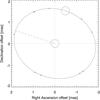 |
Fig. 1 Apparent orbit of 41 Eridani. The dashed line indicates the ascending node. The small circles outline the stellar disks. The short (red) lines connect the measurements with the orbital model values. |
To visualize the constraints provided by the interferometric observations, the data of each night were fit with relative astrometric positions (using the values for component diameters and relative flux from the all-night fit). The results are plotted on the orbit in Fig. 1. More details are given in Table 1 and include separation ρ and position angle θ (Cols. 5 and 6), the semi-major axes of the astrometric uncertainty ellipses (in Cols. 7 and 8), the position angle of the major axis (Col. 9), and the offsets of the astrometric positions from the orbit in separation and angle (Cols. 10 and 11). The astrometric uncertainty ellipses correspond in size to the synthesized point spread functions (based on the achieved interferometric aperture coverage) divided by 40 to normalize the total astrometric reduced χ2 to unity. The scaling factor is a function of the uncertainties of the visibility and closure phase measurements, which were similar for all data sets.
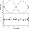 |
Fig. 2 Radial velocities from Hubrig et al. (2012) for components A (circles) and B (plus symbols) with the solid line showing the orbital model for A and the dashed line for B. The lower panel shows the fit residuals. |
4. Discussion
According to Paddock (1915), 41 Eridani “was placed in the spectral Class B9A4 in the catalogue of southern spectra given in Harvard Annals, Vol. 28, Part 2”. Paddock (1915) discusses the classification based on the fact that the star still shows helium lines, while at the same time displaying significantly more prominent metal lines compared to λ Centauri, a “typical” star of class B9. Initially, as the two components of 41 Eri appear nearly identical, we adopted the same spectral type of B9V for both of them in order to obtain photometric estimates for the apparent diameters of the stars. We used the sedFit (Boden 2007) tool to retrieve photometric data from the Simbad database, dividing the fluxes in half, and to fit stellar template spectra from Pickles (1998) to derive the bolometric flux (Fig. 3). The fit was significantly better with a template of a B8V star. Using Eq. (6) of Boden (2007),  , with the Boltzmann constant σ, an angular diameter θ = 0.36 ± 0.06 mas is fitted with a bolometric flux FBol = 8.31 × 10⁻⁷ erg cm-2 s-1, based on an effective temperature of the template of 11 750 ± 1000 K. This value is consistent with the diameter fit to the interferometric data (given in Table 2).
The effective temperatures derived from spectroscopy by Dolk et al. (2003), Teff,A = 12 750 K and Teff,B = 12 250 K, uncertainty of 200 K, are higher still and would correspond to spectral types between B8 and B7 (Aller et al. 1982). Owing to the smaller uncertainty of the spectroscopic effective temperatures, we adopt these in the following. Using again equation 6 of Boden (2007), θ = 8.17 mas × 10− 0.2(V + BC)(Teff/ 5800 K)-2, nearly identical angular diameters of 0.35 ± 0.01 mas are obtained for each component with the bolometric corrections BCA = −0.84 and BCB = −0.73 (Flower 1996; Torres 2010). Here we adopted the same magnitude difference in the V band as measured in the H band by PIONIER to compute individual component magnitudes from the combined V = 3.56 (Simbad). The corresponding luminosities are given in Table 2 together with the log g values, which are computed from the masses and absolute stellar radii of 2.32 ± 0.18 R⊙. Dolk et al. (2003) derived log g = 4.18 ± 0.10 for the primary and log g = 4.10 ± 0.10 for the secondary from uvby photometry; the latter value is smaller owing to the lower Teff.
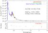 |
Fig. 3 Fit of apparent diameter (and effective temperature) to Simbad photometry with sedFit. The red symbols correspond to the photometric data and the green crosses to the model values. The blue line denotes the template from Pickles (1998) for a B8 main-sequence star. The (reduced) χ2 of the fit is given in the figure as well. The lower panel shows the fit residuals as fractions of the total flux. |
We show in Fig. 4 the stellar evolutionary tracks of two stars with solar metallicity interpolated for masses of the primary and secondary of 41 Eridani using models of Ekström et al. (2012). The average age of the model stars matching all observables best is 50 ± 2 Myr, and their average radius is 2.1 ± 0.1 R⊙, which is consistent with the values quoted in Table 2. The stars are therefore slightly evolved and the average model surface gravity is log g = 4.3.
The rotational rate of the stars was measured to be the same (vsini = 12 km s-1) by Dolk et al. (2003) and translates into an equatorial velocity of 22 km s-1 (assuming spin-orbit alignment). If we divide the stellar circumference derived from the angular diameter and the distance (10.1 ± 0.8 × 10⁶ km) by the orbital period, we obtain an equatorial velocity of 23.4 ± 1.8 km s-1, which is consistent with the value derived from the rotational rate and therefore indicates synchronous corotation of the stars.
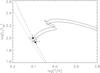 |
Fig. 4 Stellar evolutionary tracks (solid lines) for solar composition stars of 3.15 M⊙ and 3.07 M⊙, based on models by Ekström et al. (2012). The two large symbols represent the observations with error bars in luminosity and effective temperature, while open circles indicate the models closest to the observations. The dashed line is an isochrone for the age of 50 Myr with solid circles indicating models closest to the observed stars. The dotted line is the zero-age main sequence. |
5. Summary
Observations of the spectroscopic binary 41 Eridani were performed with the PIONIER H-band beam combiner at the VLTI and allowed the component separation to be resolved at each of the 10 epochs thanks to the high-precision data delivered by this instrument. The elements of the five-day apparent orbit were derived and, when combined with those of the spectroscopic orbit (Hubrig et al. 2012), delivered the stellar masses with an accuracy of 2% and the orbital parallax with an accuracy of 1%. The diameters of the nearly identical components, while barely resolved, were consistent with estimates based on fitting the spectral energy distribution. The derived effective temperature was higher than expected for a main-sequence star with spectral classification B9, confirming results by Dolk et al. (2003), and might be related to an erroneous classification in the Harvard Annals due to the stronger metal lines of this chemically peculiar star.
The letter A was used by Cannon & Pickering (1901) to indicate the adjacent spectral class.
Acknowledgments
The authors want to warmly thank all the people involved in the VLTI project and Jean-Baptiste Le Bouquin and the PI Team for their contributions to PIONIER and the science-grade pipeline. This article made use of the Smithsonian/NASA Astrophysics Data System (ADS), of the Centre de Données astronomiques de Strasbourg (CDS), and of the Jean-Marie Mariotti Center (JMMC). We thank Gerard van Belle for providing an installation of sedFit. We thank the anonymous referee for comments that helped improve our paper.
References
- Abt, H. A., Chaffee, F. H., & Suffolk, G. 1972, ApJ, 175, 779 [Google Scholar]
- Aller, L. H., Appenzeller, I., Baschek, B., et al. 1982, Landolt-Börnstein: Numerical Data and Functional Relationships in Science and Technology − New Series. Group 6 Astronomy and Astrophysics, Vol. 2 [Google Scholar]
- Boden, A. F. 2007, New Astron. Rev., 51, 617 [NASA ADS] [CrossRef] [Google Scholar]
- Cannon, A. J., & Pickering, E. C. 1901, Ann. Harvard College Obs., 28, 129 [NASA ADS] [Google Scholar]
- Catanzaro, G., & Leto, P. 2004, A&A, 416, 661 [NASA ADS] [CrossRef] [EDP Sciences] [Google Scholar]
- Cole, W. A., Fekel, F. C., Hartkopf, W. I., McAlister, H. A., & Tomkin, J. 1992, AJ, 103, 1357 [NASA ADS] [CrossRef] [Google Scholar]
- Dolk, L., Wahlgren, G. M., & Hubrig, S. 2003, A&A, 402, 299 [NASA ADS] [CrossRef] [EDP Sciences] [Google Scholar]
- Ekström, S., Georgy, C., Eggenberger, P., et al. 2012, A&A, 537, A146 [NASA ADS] [CrossRef] [EDP Sciences] [Google Scholar]
- Flower, P. J. 1996, ApJ, 469, 355 [NASA ADS] [CrossRef] [Google Scholar]
- Gallenne, A., Mérand, A., Kervella, P., et al. 2015, A&A, 579, A68 [NASA ADS] [CrossRef] [EDP Sciences] [Google Scholar]
- González, J. F., Hubrig, S., Nesvacil, N., & North, P. 2006, A&A, 449, 327 [NASA ADS] [CrossRef] [EDP Sciences] [Google Scholar]
- González, J. F., Hubrig, S., & Castelli, F. 2010, MNRAS, 402, 2539 [NASA ADS] [CrossRef] [Google Scholar]
- Hubrig, S., & Mathys, G. 1995, Comments on Astrophysics, 18, 167 [Google Scholar]
- Hubrig, S., & Mathys, G. 1996, A&AS, 120, 457 [NASA ADS] [CrossRef] [EDP Sciences] [Google Scholar]
- Hubrig, S., Savanov, I., Ilyin, I., et al. 2010, MNRAS, 408, L61 [NASA ADS] [CrossRef] [Google Scholar]
- Hubrig, S., González, J. F., Ilyin, I., et al. 2012, A&A, 547, A90 [NASA ADS] [CrossRef] [EDP Sciences] [Google Scholar]
- Isobe, S. 1991, PASA, 9, 270 [NASA ADS] [CrossRef] [Google Scholar]
- Lafrasse, S., Mella, G., Bonneau, D., et al. 2010, VizieR Online Data Catalog, II/300 [Google Scholar]
- Le Bouquin, J.-B., Berger, J.-P., Lazareff, B., et al. 2011, A&A, 535, A67 [NASA ADS] [CrossRef] [EDP Sciences] [Google Scholar]
- LeBouquin, J.-B., Beust, H., Duvert, G., et al. 2013, A&A, 551, A121 [NASA ADS] [CrossRef] [EDP Sciences] [Google Scholar]
- Paddock, G. F. 1915, Lick Observatory Bull., 8, 168 [NASA ADS] [CrossRef] [Google Scholar]
- Pan, X., Shao, M., Colavita, M. M., et al. 1992, ApJ, 384, 624 [NASA ADS] [CrossRef] [Google Scholar]
- Pickles, A. J. 1998, PASP, 110, 863 [CrossRef] [Google Scholar]
- Renson, P., & Manfroid, J. 2009, A&A, 498, 961 [NASA ADS] [CrossRef] [EDP Sciences] [Google Scholar]
- Sana, H., Le Bouquin, J.-B., Lacour, S., et al. 2014, ApJS, 215, 15 [NASA ADS] [CrossRef] [Google Scholar]
- Schöller, M. 2007, New Astron. Rev., 51, 628 [NASA ADS] [CrossRef] [Google Scholar]
- Schöller, M., Correia, S., Hubrig, S., & Ageorges, N. 2010, A&A, 522, A85 [NASA ADS] [CrossRef] [EDP Sciences] [Google Scholar]
- Shulyak, D., Paladini, C., Causi, G. L., Perraut, K., & Kochukhov, O. 2014, MNRAS, 443, 1629 [NASA ADS] [CrossRef] [Google Scholar]
- Torres, G. 2007, AJ, 133, 2684 [NASA ADS] [CrossRef] [Google Scholar]
- Torres, G. 2010, AJ, 140, 1158 [NASA ADS] [CrossRef] [Google Scholar]
- van Leeuwen, F. 2007, A&A, 474, 653 [NASA ADS] [CrossRef] [EDP Sciences] [Google Scholar]
- Wittkowski, M., Schöller, M., Hubrig, S., Posselt, B., & von der Lühe, O. 2002, Astron. Nachr., 323, 241 [NASA ADS] [CrossRef] [Google Scholar]
- Wolff, S. C., & Wolff, R. J. 1974, ApJ, 194, 65 [NASA ADS] [CrossRef] [Google Scholar]
- Zavala, R. T., Adelman, S. J., Hummel, C. A., et al. 2007, ApJ, 655, 1046 [NASA ADS] [CrossRef] [Google Scholar]
All Tables
All Figures
|
Fig. 1 Apparent orbit of 41 Eridani. The dashed line indicates the ascending node. The small circles outline the stellar disks. The short (red) lines connect the measurements with the orbital model values. |
| In the text | |
|
Fig. 2 Radial velocities from Hubrig et al. (2012) for components A (circles) and B (plus symbols) with the solid line showing the orbital model for A and the dashed line for B. The lower panel shows the fit residuals. |
| In the text | |
|
Fig. 3 Fit of apparent diameter (and effective temperature) to Simbad photometry with sedFit. The red symbols correspond to the photometric data and the green crosses to the model values. The blue line denotes the template from Pickles (1998) for a B8 main-sequence star. The (reduced) χ2 of the fit is given in the figure as well. The lower panel shows the fit residuals as fractions of the total flux. |
| In the text | |
|
Fig. 4 Stellar evolutionary tracks (solid lines) for solar composition stars of 3.15 M⊙ and 3.07 M⊙, based on models by Ekström et al. (2012). The two large symbols represent the observations with error bars in luminosity and effective temperature, while open circles indicate the models closest to the observations. The dashed line is an isochrone for the age of 50 Myr with solid circles indicating models closest to the observed stars. The dotted line is the zero-age main sequence. |
| In the text | |
Current usage metrics show cumulative count of Article Views (full-text article views including HTML views, PDF and ePub downloads, according to the available data) and Abstracts Views on Vision4Press platform.
Data correspond to usage on the plateform after 2015. The current usage metrics is available 48-96 hours after online publication and is updated daily on week days.
Initial download of the metrics may take a while.